Lithostratigraphic Classification Method Combining Optimal Texture Window Size Selection and Test Sample Purification Using Landsat 8 OLI Data
-


Abstract
Gray Level Co-Occurrence Matrix (GLCM), as a measure of spatial features has been used as supplemental information to improve image classification accuracy for lithological recognition. Window size is an important parameter for texture extraction, which will affect the extracted texture results. Besides, the existence of mixed pixels in image usually causes errors in test samples, which significantly influences the credibility of accuracy assessment. Thus, this paper proposes a lithological classification method combined with optimal texture window size selection and test sample purification. Firstly, optimal window size pre-estimated based on semivariogram was used to calculated GLCM texture of image. Secondly, based on multidimensional textural and spectral features, a support vector machine (SVM) classifier was employed to classify the image. Thirdly, using the proposed sample purification method and textural features of image, sample purification rules were created based on attribute coherence to remove the test sample points that conflicted with the rules. Finally, the validity of the semivariogram-based texture extraction window selection was verified by classifications based on Angular Second Moment (ASM) of different window sizes combined with spectral features. Also, the accuracies between different combinations of classifications were assessed by test samples with and without sample purification. Experimental results show that the pre-estimated texture window size can guarantee a classification result with high classification accuracy for lithological classification. The results also demonstrated that the accuracy of lithological classification based on spectral features and ASM textural features was the highest. The overall lithological classification accuracy and kappa value, without sample purification selected by stratified sampling, were respectively 87.4% and 0.84, however those with sample purification were respectively 88.01% and 0.85. The results show that the proposed method is capable of yielding more reliable lithostratigraphic identification.
1 Introduction
Lithostratigraphic classification is one of the most common fields in geology for application of remote sensing. Many studies have demonstrated that exploiting the spectral characteristics of minerals and rocks can effectively accomplish lithostratigraphic identification and mineral detection. The lithological information extraction approaches, based on spectral features, mainly focus on the conversion and enhancement of spectral features. These approaches include principal component analysis (PCA), matched-filtering, spectral angle mapping (SAM), band gap ratio (BR), relative absorption band depth (RBD), false color composite (FCC), and combinations of these methods [1, 2, 3, 4, 5, 6, 7, 8, 9, 10]. For example, based on visible light near-infrared (VNIR) and short-wave infrared (SWIR) bands of ASTER data, using the matching-filter, can identify limestone and dolomite; whereas the quartz rock and carbonate rocks can easily be identified through using the thermal infrared band (TIR) [11].
Due to local changes in mineral composition, terrain, vegetation cover, weathering, and other factors, spectral features within the same lithology category may have significant differences, and different rock types may have similar spectral features. Therefore, using only spectral features from the image for lithostratigraphic classification may limit accuracy. Thus, numerous studies have tried to add texture information for lithostratigraphic recognition to achieve higher accuracy. Texture feature is a visual feature that reflects the homogeneity of the image without depending on color or brightness, which are internal features of object surface [12]. Texture features contain important information about the organization of an object’s surface structure and contacts of the object with its surrounding environment [13]. Existing studies have shown that image texture features incorporated into lithostratigraphic classification can effectively improve classification accuracy [14, 15, 16, 17, 18, 19]. Very accurate results in lithostratigraphic classification achieved when spectral features and Gray Level Co-Occurrence Matrix (GLCM) textural features were used together as noted by Mather et al. [20]. Subsequent studies also demonstrated the usefulness of GLCM for lithostratigraphic classification.
Window size is an important parameter for texture extraction process, too large or too small size will not be ideal for texture extraction. Semivariogram is a function of the distance between samples and the semivariance of samples. This feature spatially represents a spatial autocorrelation, reflected the spatial relationship between pixels on the image. The semivariogram method has been widely used to scale selection of remote sensing image segmentation [21]. In this paper, the optimal texture window size is estimated using semivariance, and the effectiveness of the method is verified by taking classification based on ASM of different window sizes and spectral features as an example.
Selecting an appropriate classification algorithm is an important step in determining the overall classification success [22]. Support vector machine (SVM), a nonparametric classifier, is a good performance classifier with the ability to handle multiple effective image features even though the sample size is small [22]. The known effective SVM algorithm can be applied to high-dimensional data to avoid dimension issues. Moreover, the categories of seven rocks are linearly unseparable in feature space, many lithostratigraphic classification studies have demonstrated that the SVM classifier has good lithostratigraphic identification and classification performance [23, 24, 25, 26, 27, 28, 29, 30, 31]. In this study, because we attempt to combine multiple spectral and textural features for lithostratigraphic classification, the SVM algorithm is an appropriate selection.
Remote sensing image classification accuracy assessment is an absolutely necessary link in remote sensing classification technology. Accuracy assessment can effectively evaluate the classifier, and can also provide the final evaluation of image classification results [32]. Accuracy assessment can also provide an evaluation of the quality of classification for users [33], and therefore has important significance for application in remote sensing classification. Numerous researchers have studied remote sensing image classification accuracy assessments. Currently, the factors that affect accuracy assessment include three aspects: sampling design, reference data, and evaluation parameters [34]. Among them, sampling design is the most critical aspect, which not only determines the cost of the accuracy assessment, but also constitutes the basis of the accuracy assessment [35, 36, 37]. The reference data, mainly confined to reality and cost, will affect the quality of the test samples. The widely-used evaluation parameters contain overall accuracy (OA), kappa coefficient, producer’s accuracy (PA), and user’s accuracy (UA). In addition, Pontius and Millones [38] have proposed two evaluation parameters, quantity disagreement and allocation disagreement, that can describe the information in a confusion matrix and express classification accuracy better. These evaluation parameters are outputs of the confusion matrix.
Sampling design has a significant influence on deriving the confusion matrix. The sampling design process needs to consider three parts: sampling unit, sample set size, and sampling method [36]. The sampling unit contains point and polygon units. The sample set size means the number of test samples will affect the accuracy assessment results [39, 40, 41]. The sampling method includes simple random, stratified, and systematic sampling [40, 42]. In the process of selecting test samples, the existence of mixed pixels in the image and artificial error may cause misclassified samples, so that test samples may have errors. In the process of accuracy assessment, however, the error in test samples is often neglected, and all the errors are associated to classification error, which makes the assessment results unreliable. Therefore, this paper suggests that before accuracy assessment, test samples should be purified to reduce this error, which will make assessment results more objective and unbiased.
This paper uses semivariogram to pre-estimate the optimal window size for texture extraction and notes a key problem in an accuracy assessment program, the quality of test samples, and subsequently proposes a method which depends on the feature information to purify test samples and reduce its error. The effectiveness of optimal texture window size selection method and test sample purification technique are verified by experiments. This study used the Landsat 8 operational land imager (OLI) data, which can recognize rocks well [19, 43, 44, 45] and can be obtained free from the United States Geological Survey (USGS) and Earth Resources Observation and Science (EROS) data [46].
2 Methodology
2.1 Workflow of Lithostratigraphic Classification
The workflow for this method comprises several stages shown in Figure 1. The main stages are: semivariogram based optimal texture window size selection, GLCM based textural features extraction, SVM based lithostratigraphic classification, test sample set size calculation and selection, sample purification rules creation based on textural information of training samples and purified test samples, accuracy assessment based on test samples with sample purification, and results analysis.
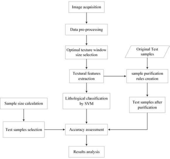
Flowchart of the lithostratigraphic classification method combining optimal texture window size selection and test sample purification technique
2.2 Semivariogram-based Window Size Selection for Texture Extraction
The semivariogram proposed by Matheron [47] is a spatial statistical method. The semivariogram can show how the variance of a variable varies with different sampling intervals on one image, which can represent the degree or scale of spatial variability. Semivariance γ(h) is determined by Equation (1) [21].
where h is the lag (or spatial sampling interval) and is a vector in both distance and direction because of the existence of anisotropy. X( i) is a sample value at location i, and X(i+h) is another sample value separated from X(i) with the sample interval h. N(h) is the total amount of pairs of X(i) and X(i+h).
The increasing and second derivative of semivariance are calculated from Equation (2) [21] and (3) [21] respectively.
where [Δγ(h)i] is the increasing of semivariance and [γ''(h)i] is the second derivative of semivariance, i represents the calculating times of the semivariogram with different sampling intervals.
The range of semivariogram (threshold of autocorrelation) associates the feature scale of the landscape. Within the range, the autocorrelation exists among variables, while beyond the range, autocorrelation may be untenable. So the range can be deemed as the measurement of similarity between variables, and it can indicate the size of a spatial object, a spatial phenomenon or a spatial pattern, as well as the size of texture primitive. So the range of semivariogram can be used to estimate the optimal texture window size. More specifically, the range is set as the sampling interval hi corresponding to [Δγ(h)i] whose value is first less than or equal to zero with the increasing of h and [γ"(h)i] whose value is first greater than or equal to zero with the increasing of h. More details, please refer to Section 4.1.
2.3 Principles of Textural Feature Expression Based on GLCM
GLCMis a common method for describing texture by studying the spatial correlation of pixel gray. As a statistical method, it has been widely used to extract the features of texture statistics from images. Based on GLCM, Haralick [13] proposes 14 textural features to extract from the texture statistics of images. Commonly used features for lithostratigraphic classification include Angular Second Moment (ASM), Homogeneity (Homo), Entropy (Ent), Correlation (Cor), and Contrast (Con) [48, 49]. In this study, taking into account the time consumption, four important features, ASM, Ent, Cor, and Con, are selected for extracting textural features of the study area.
ASM, known as Uniformity or Energy, is the sum of squares of the elements value in the GLCM [48]. It reflects gray scale distribution uniformity and texture roughness of the image [50]. ASM is high when the image is a uniform and regularly changing texture pattern. ASM is extracted by Equation (4) [51].
Ent, determined by Equation (5) [48], shows the complexity of the image [50]. The higher the Ent, the more complex image [48].
Cor, calculated by Equation (6) [48], measures the dependency of grey levels in the row or column direction [15]. Therefore, it reflects the correlation between local grey levels [52]. Cor is high when grey levels of an image are even [50].
Con, extracted by Equation (7) [51], measures the distribution of values in the GLCM and local changes in the image [15]. It reflects the clarity of the image and the depth of the textural grooves [53]. Con is high when the textural groove is deep, and the image is clear; the Con is low when the textural groove is shallow, and the image is fuzzy [50].
Where P(i,j|d,θ) is a GLCM with step size d and angle θ, (i, j) means position. μx, μy, σx, and σy are the means and standard deviations of rows and columns.
For this paper, the step sizes of one and direction of 45∘ were set for computing the P(i,j|d,θ). The window size is selected by semivarogram. Then, according to Equations (4)–(7), ASM, Ent, Cor, and Con can be extracted.
2.4 Support Vector Machine Classifier
The SVM studied by Vapnik et al. [54, 55, 56, 57] is a supervised machine learning algorithm which is based on statistical learning theory. The SVM seeks a hyperplane that satisfies the classification requirements, and ensures the distance between the training data and hyperplane is as far as possible. The learning strategy of SVM is through interval maximization, which is applied to convex quadratic programming problem solving.
The rationale of SVM can be summarized as follows [58]:
Map the points in low-dimensional space into high-dimensional space based on the kernel function, so that they become linearly separable.
Use the principle of linear division to determine the optimal hyperplane which can separate the two classes correctly, and the classification margin is at the maximum. The classification margin is the gap between the hyperplane and the closest training samples. The closest training samples are support vectors.
The optimal classification function is [58]:
where {(X1, y1),(X2, y2),...,(Xn, yn)} are training samples, Xi∈ Rn, yi∈ (-1,1). X = (X1, X2,..., Xn) means the input vectors, Xi(i = 1,2,..., N) are support vectors. ai and b are undetermined coefficients of the hyperplane. K(X, Xi) is the kernel function including Linear, Polynomial, Radial Basis Function (RBF), and Sigmoid Kernel. The Radial Basis Function is chosen for this study.
2.5 Accuracy Assessment Combining Test Sample Purification
2.5.1 Sample Set Size
For simple random sampling, an appropriate test sample size could be estimated by Equation (9) [59].
where Ois the estimated overall accuracy that we expect to achieve, z is the value from the standard normal distribution corresponding to the confidence level (z = 1.96 corresponding to a 95 %confidence level, z = 1.645 corresponding to a 90 %confidence level) and d is the allowable range of error for the confidence interval of O.
For stratified sampling, we assumed the sampling cost of every class is the same, and an appropriate test sample size could be calculated from Equation (10) [59] and (11) [59].
where
where N is the number of pixels in the study area, S(Ô) is the standard error of the targeting overall accuracy, Wi is the occupied ratio of area by class i, Si is the standard deviation of class i, calculated from Equation (11), and Ui is the user’s accuracy of class i.
2.5.2 Sample Purification
A confusion matrix based on good test samples could more objectively depict classification accuracy. Therefore, before using test samples to assess accuracy, sample purification of test samples is necessary to ensure the credibility of the lithostratigraphic classification accuracy. The method of sample purification is based on attribute coherence, which means for the same class the test samples would have similar properties as the training data. The attribute contains both spectral and textural features. Therefore, it is necessary to select appropriate attributes to identify different classes.
The method used to establish sample purification rules are:
where Pij is the sample purification rule of class i based on feature j, i and j represent different classes and different features, Test_Fij and Training_Fij mean the value of feature j for test sample and training sample of class i. The min(Training_Fij) and max(Training_Fij) represent minimum and maximum values of feature j for the training sample of class i. Features contain spectral and textural features in this method.
For training samples of class i, if its median value of feature j is the largest and the gap between the other categories is also the largest, we will use Equation (12) to obtain Pij; conversely, if the median value of feature j is the smallest and the gap between the other categories is also the largest, Equation (13) will be applied to derive Pij. In addition, the rest of the classes correspond to Equations (12) and (13).
The process of sample purification is as follows:
Compute the features information for training samples of each class, and draw a chart based on the median values of the features;
According to the chart, determine to use either Equation (12) or Equation (13) to create and establish sample purification rules;
Purify the test samples, according to the rules derived from step two to exclude the sample points that conflict with the rules.
3 Study Area and Data
3.1 Study Area
The study area (Figure 2) is located in the northwest margin of the Tarim Basin, which lies in the Xinjiang province of Western China, with an eastern longitude range from 77∘35' to 78∘10' and a northern latitude range from 40∘0' to 40∘25'. The average elevation of the study area is approximately 1885 m. The region has a temperate-continental climate, resulting in low precipitation, poor vegetation development, and good rock outcrops, which is the ideal area for using satellite remote sensing technology for geological research. The main stratigraphic units in this area include Є-O, S, D, C-P, N2, Q1, Q3−4 [60]. The 1:200,000 geological map (Xinjiang Geological Survey, 1965a, b) of the area was used as the reference map [60], shown in Figure 3. Main rock units in the study area and their lithostratigraphic description are shown in Table 1.

Location of study area.

The lithostratigraphic map of the study area.
Description of lithostratigraphic units in the study area.
| Rock Units | Local Name of Rock Units | Geological Time | Lithological Description |
|---|---|---|---|
| Є-O | Qiulitage Group | Cambrian | Dolomite and gray stratified limestone |
| S | Kepingtage Group | Ordovician | Gray-green mudstone; quartz siltstone; muddy siltstone; gray-green sandstone; yellow-gray bottom sandstone |
| D | Shalayimu Group | Silurian | Light green, red, purple-brown sandstone; flood layer |
| C-P | Kangkelin and Bieliangjin Groups | Devonian | Light gray, gray-red, gray limestone; gray-black sandstone |
| N2 | Cangzongse Formation | Carboniferous | Flood pale-brown layer; pale-mudstone; brown pale-sandstone; brown siltstone |
| Q1 | - | Tertiary | Flood layer |
| Q3−4 | - | Quaternary | Sandy soil; sandy clay |
3.2 Data and Data Pre-processing
The image used in the present study was acquired by Landsat 8 OLI on July 30, 2013. The data (LC81480322013211LGN00), was provided by USGS EROS data center [46]. The image has 0.75% of cloud cover, which mainly concentrated in the upper corner. Therefore, no cloud was presented in the image of study area, as shown in Figure 4. Figure 4 shows the false color composition of the study area. The study uses the multispectral and panchromatic data of the image, which are detailed in Table 2. The images we obtained are Level-1 digital number data products that have been radiometrically and geometrically corrected by USGS. The images were processed as follows:

Landsat 8 false color composite image of the study area (R = band 5 (NIR, 0.845–0.885), G = band 4 (Red, 0.630–0.680), and B = band 3 (Green, 0.525–0.600)).
Landsat 8 Operational Land Imager (OLI) band information.
| Band Name | Wavelength (μm) | Spatial Resolution (m) |
|---|---|---|
| Band 1 Coastal | 0.433–0.453 | |
| Band 2 Blue | 0.450–0.515 | |
| Band 3 Green | 0.525–0.600 | |
| Band 4 Red | 0.630–0.680 | 30 |
| Band 5 NIR | 0.845–0.885 | |
| Band 6 SWIR 1 | 1.560–1.660 | |
| Band 7 SWIR 2 | 2.100–2.300 | |
| Band 8 Pan | 0.500–0.680 | 15 |
Radiometric calibration was conducted for VNIR–SWIR images to acquire the top of atmosphere reflectance data.
FLAASH atmospheric correction with the Mid-Latitude Summer atmospheric model and the rural aerosol model were conducted for the top of atmosphere reflectance data to acquire the surface reflectance data.
For ease of visually interpretation and enhancing the separability between different category, the surface reflectance data were fused with the panchromatic band by Gram-Schmidt Pan Sharpening.
C-correction, a topographic correction method based on the linear relationship between the image pixels and the cosine of the solar relative incidence angle [61], was conducted for the images to remove the shadows effect. ASTGTM DEM (Figure 5) with 30 m spatial resolution was used in Topographic Correction process.

ASTGTM DEM of the study area.
After data pre-processing, the fused VNIR–SWIR bands were used to extract texture features. All the procedures of data processing in this section were conducted in ENVI 5.1.
3.3 Vegetation Elimination in Remote Sensing Images
A small amount of vegetation was present in the used image, which needs to be considered, as shown in Figure 4. In this figure, the vegetation is shown in magenta. The texture features are described based on the spatial variability associated with the digital number (DN) of the local pixels. Therefore, the vegetation in the image will hide or damage the texture information. In order to remove vegetation, Equation (14) [62, 63] was used to calculate the normalized difference vegetation index (NDVI). In this paper, the NDVI threshold is set to 0.3, marking off the vegetation pixels, which in Figure 6 is green.

Vegetation pixels in green with 0.3 < normalized difference vegetation index (NDVI) < 1.0.
4 Experiments
4.1 Window Size Selection for Texture Extraction
As shown in Figure 7(a), the representative sampling area with a size of 600 × 600 pixels is used for calculating semivariance in this experiment. In order to accurately reflect the variation of semivariance along the spatial sampling distance, the lags are set from 3 to 45, and the step of the lag is set as 2. Band 6 with the largest standard deviation, contains the maximum amount of information. To reduce the amount of computation, the semivariograms in the horizontal and vertical directions are calculated by band 6 of the sampling area images. The synthetic semivariances are the average of the horizontal and vertical semivariograms, displayed in Figure 7(b).

(a) the sampling area with a size of 600 × 600 pixels; and (b) synthetic semivariograms.
From Figure 7(b), it can be seen that the range of the synthetic semivariogram is not obvious. To achieve pre-estimation of the reasonable window size for texture extraction, the increasing of the synthetic semivariance [Δγ(h)i] and second derivative of the synthetic semivariance [γ''(h)i] are displayed in Figure 8(a) and (b). According to Figure 8, the sampling distance for the image shown in Figure 8(a) is 11, corresponding to a 23 × 23 spatial window, and the sampling distance for image shown in Figure 8(b) is 15, corresponding to a 31 × 31 spatial window. By employing the texture window size pre-estimation method proposed in Section 2.2, the theoretical optimal texture window size is determined as 31 × 31.

Computed results of: (a) the increase of the synthetic semivariance; (b) the second derivative of the synthetic semivariance.
4.2 Spatial Textural Feature Analysis
4.2.1 Spatial Textural Feature Extraction
According to Figure 8, the texture extraction window size of 31 × 31 is used for extracting Ent, Cor, and Con. According to seven bands of Landsat 8 data, four textural features of GLCM, ASM, Ent, Cor, and Con, were calculated to obtain 28 texture images. In order to study the effectiveness of the different texture images for lithostratigraphic identification and create sample purification rules, the texture values of the training samples were extracted from the texture images. The median texture value of each category is shown in Figure 9.

Median texture value for the seven rock types: (a) median ASM value; (b) median Ent value; (c) median Cor value; and (d) median Con value. TFi means the texture images were derived from spectral band i.
Figure 9 provides the following information:
The ASM feature distinguishes Q3−4 from other rock types well, and the value calculated from band 5 is largest. Q3−4 is generally larger on ASM values, which may be because its texture is more uniform and regular-changing than other rock types.
N2 has the highest Ent value, which indicates its surface is most complex. Q3−4 has the lowest Ent, TF5, and TF6 values, which means it is simpler than other rocks.
The Cor feature can separate Q1from other rocks. The Cor values of Q1 are relatively small, which means Q1 has a small local correlation on the image. Cor values curves of S and Q3−4 fluctuate greatly, which may due to the fact that texture images derived from different bands have a variable effect on rock identification [19].
N2 shows a significant difference in the Con feature compared to other rock types, which may result from its deep textural trench. From TF1 to TF7, between the Con values, there is an obvious difference between Є-O and C-P, and the between S, D, and Q1.
In short, the application of GLCM textural features to the classification process can help improve the separation of different rock types. For the same texture, the texture images obtained from different bands have different sensitivities for rock identification. The different textures calculated in the same band have different sensitivities for lithostratigraphic identification as well. For example, an ASM image derived from band 5 distinguishes Q3−4 from other rock types, however, Ent and Con images calculated from band 5 separate N2 well. Overall, different texture images have abilities to identify different rocks.
4.2.2 Feature Selection
In this paper, we treat seven spectral bands as a whole, for ASM, Ent, Cor, and Con also. Then, the spectral and texture are combined in the SVM classifier for lithostratigraphic classification. As shown in Table 3, a total of 15 combinations of spectral and texture features are possible. Optimum Index Factor (OIF) [64] is calculated for combinations in Series 2 and Series 3 to select the optimal combinations. The correlation between band 1 and the texture features, with the standard deviation of them, is used to calculate the index. The correlation matrix between band 1 and the texture features calculated from band 1 is presented in Table 4.
Different combinations of spectral and textural features
| Series 1 | Series 2 | Series 3 | Series 4 |
|---|---|---|---|
| SF+ ASM | SF+ ASM+ Ent | SF+ ASM+ Ent+ Cor | SF+ ASM+ Ent+ Cor+ Con |
| SF+ Ent | SF+ ASM+ Cor | SF+ ASM+ Ent+ Con | - |
| SF+ Cor | SF+ ASM+ Con | SF+ ASM + Cor+ Con | - |
| SF+ Con | SF+ Ent+ Cor | SF+ Ent+ Cor+ Con | - |
| - | SF+ Ent+ Con | - | - |
| - | SF+ Cor+ Con | - | - |
Correlation matrix between band 1 and the texture features calculated from band 1. TF1 means the texture features were derived from spectral band 1; Stdev is the abbreviation of the standard deviation.
| Band 1 | ASM (TF1) | Ent (TF1) | Cor (TF1) | Con (TF1) | Stdev | |
|---|---|---|---|---|---|---|
| Band 1 | 1.00 | -0.84 | 0.79 | -0.56 | 0.21 | 508.74 |
| ASM (TF1) | 0.21 | -0.34 | 0.44 | -0.25 | 1.00 | 0.42 |
| Ent (TF1) | 0.79 | -0.94 | 1.00 | -0.66 | 0.44 | 1.69 |
| Cor (TF1) | -0.84 | 1.00 | -0.94 | 0.74 | -0.34 | 0.32 |
| Con (TF1) | -0.56 | 0.74 | -0.66 | 1.00 | -0.25 | 11.32 |
In Series 2, SF+ Ent+ Con has the largest OIF value, and the second largest is SF+ Cor+ Con. For Series 3, the optimal combination is selected by calculating the OIF index of texture feature combinations. For example, for SF+ ASM+ Ent+ Cor, we calculate the OIF index of ASM+ Ent+ Cor. And Ent+ Cor+ Con has the largest OIF value. Therefore, based on band 1, optimal selection of Series 2 and Series 3 are respectively SF+ Ent+ Con and SF+ Ent+ Cor+ Con. Wei et al. [19] demonstrated that using textural features extracted from multiple spectral bands has a better performance than that from a single spectral band to aid spectral information for lithostratigraphic classification. Hence, combinations of spectral and texture features for lithostratigraphic classification is shown in Table 5.
Combinations of texture and spectral images classified by SVM.
| Combinations | SF | ASM | Ent | Cor | Con | Overall Feature Amounts |
|---|---|---|---|---|---|---|
| C1 | SF | - | - | - | - | 7 |
| C2 | SF | ASM | - | - | - | 14 |
| C3 | SF | - | Ent | - | - | 14 |
| C4 | SF | - | - | Cor | - | 14 |
| C5 | SF | - | - | - | Con | 14 |
| C6 | SF | - | Ent | - | Con | 21 |
| C7 | SF | - | Ent | Cor | Con | 28 |
| C8 | SF | ASM | Ent | Cor | Con | 35 |
4.3 Lithostratigraphic Classification
There are seven rock types in the study area including Є-O, S, D, C-P, N2, Q1, and Q3−4, detailed in Table 1. The training sample amounts of each rock type are displayed in Table 6.
Training sample amounts for per class.
| Classes | Training Sample Amounts |
|---|---|
| Є-O | 2950 |
| S | 2189 |
| D | 1008 |
| C-P | 1106 |
| N2 | 480 |
| Q1 | 1392 |
| Q3−4 | 3057 |
| Total | 12182 |
The training samples of these rocks were selected based mainly on the reference map. Based on GLCM, four features, including ASM, Ent, Cor, and Con, were extracted. In this paper, a SVM classifier was used to classify the combinations of texture and spectral images. The combinations of texture and spectral images classified by SVM are: spectral features (SF), SF+ASM, SF+Ent, SF+Cor, SF+Con, SF+ Ent+Con, SF+Ent+Cor+Con and SF+ASM+Ent+Cor+Con, as shown in Table 5.
4.4 Accuracy Assessment Combining Sample Purification
4.4.1 Calculation of Sample Set Size
Before application, classification maps constructed from images should be assessed for accuracy [34]. An accuracy assessment process begins with sampling design. The first step in sample design is to calculate sample set size for the test samples. With z = 1.96, O = 0.74, and d = ±5 %, the resulting sample set size from Equation (9) is n = 295, marked as sample A1. Dependent on sample A1, the first accuracy assessment is carried out, and the mean user’s accuracies (Ui) are shown in Table 7.
Information needed to calculate sample size from Equation (9). The information contains the occupied area proportions (Wi), mean values of user’s accuracies (Ui), and standard deviations (Si) of the class.
| Class (i) | Wi | Ui | Si |
|---|---|---|---|
| Є-O | 0.22 | 0.80 | 0.40 |
| S | 0.11 | 0.91 | 0.29 |
| D | 0.06 | 0.90 | 0.33 |
| C-P | 0.06 | 0.47 | 0.50 |
| N2 | 0.04 | 0.50 | 0.50 |
| Q1 | 0.16 | 0.63 | 0.49 |
| Q3−4 | 0.35 | 0.94 | 0.24 |
Because N is adequately large (exceeding six million pixels in this study), for Equation (10), the second item in the denominator can be neglected. Once n is defined, proportional allocation [65] can be used to determine the sample size per strata in this paper. In addition, the stratified sampling [42, 66, 67, 68] strategy is employed and systematic sampling [36, 59] is then applied for every class. In this research, test samples select from the entire original image with step sizes of 80 pixels row by row and column by column. Table 7 provides information that is needed to calculate sample set size from Equation (10). Among them, the mapped area proportions (Wi) is the mean of all classification results. Based on Table 7, specified S(Ô) for 0.01, the sample set size calculated from Equation (10) is n = 1246, marked as sample B1. n is the overall sample set size. The allocation of the number of samples per class was determined by proportion, detailed in Table 8. When we applied sample purification rules (Table 9) to samples A1 and B1, we derived sample A2 and B2, detailed in Table 8.
Sample set size of samples A1, A2, B1, and B2; sample A1 and B1 are the original sample set; samples A2 and B2 are the sample set with sample purification.
| Class | Simple Random Sampling | Stratified Sampling | ||
|---|---|---|---|---|
| Sample A1 | Sample A2 | Sample B1 | Sample B2 | |
| Є-O | 83 | 83 | 274 | 273 |
| S | 41 | 41 | 137 | 137 |
| D | 20 | 20 | 75 | 75 |
| C-P | 19 | 19 | 75 | 70 |
| N2 | 14 | 11 | 50 | 46 |
| Q1 | 35 | 35 | 200 | 198 |
| Q3−4 | 83 | 83 | 435 | 435 |
| Total | 295 | 292 | 1246 | 1235 |
Sample purification rules.
| Class | ASM | Ent | Cor | Con |
|---|---|---|---|---|
| Є- O | 0.003<TF1-7<0.1 | - | - | - |
| S | - | - | - | - |
| D | TF1-7>0.01 | - | - | - |
| C-P | 0.01<TF1-7<0.1 | - | - | - |
| N2 | 0.003<TF1-7<0.1 | TF1-7>4 | TF1-2<0.7 | TF1-7>6 |
| Q1 | 0.005<TF1-7<0.1 | - | - | TF1-7>3 |
| Q3−4 | TF1-7>0.01 | TF5-6<5.5 | - | - |
4.4.2 Creation of Sample Purification Rules
According to problems that were mentioned in Section 1, test sample purification was implemented to improve the reliability of classification accuracy. Based on Section 2.5.2, Section 4.2, and ranges of ASM, Ent, Cor, and Con values, sample purification rules were created, detailed in Table 9.
5 Discussion
5.1 Verification of Texture Window Size Selection Method Based on Semivariogram
To verify the effectiveness of the semivariogram-based texture extraction window selection method, different ASMs with different window sizes combined with spectral features are classified by SVM. To reduce computation of verification, ASM extractions are based on window size from 5 × 5 to 41 × 41 with a step of 6. To maintain the comparability between different classification results, the training and test sample sets were the same. The test sample set used is sample B2. Table 10 demonstrates the overall accuracies (OA) and kappa with different ASM window sizes in SVM based supervised classifications.
Classification accuracies of images which ASM extracted from different windows respectively combined with spectral feature.
| Window sizes | OA | Kappa |
|---|---|---|
| 5 × 5 | 85.49% | 0.82 |
| 11 × 11 | 87.12% | 0.84 |
| 17 × 17 | 87.44% | 0.84 |
| 23 × 23 | 88.09% | 0.85 |
| 29 × 29 | 88.01% | 0.85 |
| 31 × 31 | 88.01% | 0.85 |
| 35 × 35 | 88.01% | 0.85 |
| 41 × 41 | 87.60% | 0.84 |
Table 10 shows the change in OA and Kappa with the change of ASM extraction window in SVM classifications. The highest OA is 88.09% corresponding to the texture extraction window of 23 × 23, which is just one of the pre-estimated window sizes. The second highest OA is 88.01% corresponding to the texture extraction window of 29 × 29, which is very close to the pre-estimated window of 31 × 31.
The experiment results verified that the spatial statistics-based texture window size pre-estimation is effective.
5.2 Benefit of Sample Purification
Figure 10 shows the OA and kappa of different combinations derived from test samples A1, A2, B1, and B2. As shown in the figure, the OA and Kappa obtained from the four test samples are different for the same classification result. The differences between samples A1 and B1, or samples A2 and B2 may result from the difference of sample set size and sampling method. For accuracies derived from samples A1 and A2, or samples B1 and B2, the difference may due to sample purification. The OA and Kappa derived from test samples with sample purification are higher than original test samples, because the error in the test samples that have been purified is smaller than those that have not. The error of test sample will reduce classification accuracy. After sample purification, the error of samples A2 and B2 is smaller than original test samples. Accuracies based on samples A2 and B2, which reduced the error of test samples, is more precise than that based on original test samples.

The overall accuracies (OA) and kappa of different combinations derived from test samples A1, A2, B1, and B2: (a) OA curves; (b) kappa curves. Sample A1 and B1 are the original sample set selected by simple random sampling and stratified sampling, sample A2 and B2 are the sample set with sample purification selected by simple random sampling and stratified sampling. Ci is the different combinations classified by SVM, detailed in Table 5.
Table 11 demonstrates the PA and UA of different classifications obtained from samples B1. Table 12 shows the PA and UA of different classifications obtained from samples B2. By analyzing Table 11 and 12, it can be explicitly seen that UA and PA for lithostratigraphic classification have been improved when the ASM feature is added. Regardless of whether the texture features were added or not, the recognition accuracies of S and D is relatively high. This may be due to their prominent color features. When combined with texture features, the recognition accuracy of Є-O and Q3−4 is significantly improved. It may result from their different s urface roughness, which would assist rock. For C-P and N2, their texture features are similar to Q1, and the spectral characteristics of C-P are similar to Є-O, resulted in their poor classification accuracy. Furthermore, besides UA for N2 and Q1, the rest of the features were also improved after the test samples were purified. In summary, lithostratigraphic classification combined with test sample purification i s more r eliable for lithostratigraphic identification.
The producer’s and user’s accuracies (PA and UA) of Ci classification derived from test samples without sample purification selected by stratified sampling (sample B1); Ci means different combinations classified by SVM, detailed in Table 5.
| Classes | C1(%) | C2(%) | C3(%) | C4(%) | ||||
|---|---|---|---|---|---|---|---|---|
| PA | UA | PA | UA | PA | UA | PA | UA | |
| Є-O | 73.36 | 81.05 | 83.21 | 91.57 | 85.4 | 91.76 | 85.77 | 81.6 |
| S | 97.81 | 87.58 | 95.62 | 91.61 | 94.16 | 89.58 | 91.24 | 71.43 |
| D | 98.67 | 93.67 | 97.33 | 98.65 | 89.33 | 97.1 | 86.67 | 90.28 |
| C-P | 53.33 | 45.98 | 56 | 43.3 | 54.67 | 40.59 | 64 | 42.48 |
| N2 | 52 | 44.07 | 44 | 56.41 | 44 | 68.75 | 48 | 63.16 |
| Q1 | 82.5 | 72.37 | 86.5 | 81.99 | 88.5 | 77.63 | 74 | 66.67 |
| Q3−4 | 81.61 | 90.56 | 96.55 | 97 | 93.79 | 97.84 | 73.33 | 94.38 |
| Classes | C5(%) | C6(%) | C7(%) | C8(%) | ||||
| PA | UA | PA | UA | PA | UA | PA | UA | |
| Є-O | 87.59 | 89.22 | 85.4 | 91.41 | 87.23 | 89.85 | 86.86 | 89.81 |
| S | 97.08 | 92.36 | 94.89 | 85.53 | 89.78 | 79.35 | 88.32 | 79.08 |
| D | 93.33 | 97.22 | 89.33 | 100 | 86.67 | 98.48 | 86.67 | 98.48 |
| C-P | 52 | 43.82 | 61.33 | 41.44 | 62.67 | 40.87 | 61.33 | 40 |
| N2 | 44 | 66.67 | 46 | 76.67 | 44 | 68.75 | 44 | 68.75 |
| Q1 | 85 | 77.63 | 81.5 | 75.46 | 74.5 | 80.54 | 74.5 | 80.54 |
| Q3−4 | 92.64 | 95.95 | 92.64 | 97.34 | 93.79 | 95.55 | 94.48 | 95.58 |
The producer’s and user’s accuracies (PA and UA) of Ci classification derived from test samples with sample purification selected by stratified sampling (sample B2); Ci means different combinations classified by SVM, detailed in Table 5.
| Classes | C1(%) | C2(%) | C3(%) | C4(%) | ||||
|---|---|---|---|---|---|---|---|---|
| PA | UA | PA | UA | PA | UA | PA | UA | |
| Є-O | 73.63 | 82.38 | 83.52 | 93.06 | 85.71 | 93.23 | 85.71 | 82.11 |
| S | 97.81 | 87.58 | 95.62 | 91.61 | 94.16 | 89.58 | 91.24 | 71.84 |
| D | 98.67 | 93.67 | 97.33 | 98.65 | 89.33 | 97.1 | 86.67 | 90.28 |
| C-P | 57.14 | 46.51 | 60 | 43.75 | 58.57 | 41 | 68.57 | 42.86 |
| N2 | 54.35 | 43.86 | 45.65 | 55.26 | 45.65 | 67.74 | 50 | 62.16 |
| Q1 | 82.32 | 72.44 | 86.36 | 82.21 | 88.38 | 77.78 | 74.24 | 67.74 |
| Q3−4 | 81.61 | 91.03 | 96.55 | 97.67 | 93.79 | 98.55 | 73.33 | 94.66 |
| Classes | C5(%) | C6(%) | C7(%) | C8(%) | ||||
| PA | UA | PA | UA | PA | UA | PA | UA | |
| Є-O | 87.55 | 90.53 | 85.71 | 92.13 | 87.55 | 90.53 | 87.18 | 90.49 |
| S | 97.08 | 92.36 | 94.89 | 85.53 | 89.78 | 79.35 | 88.32 | 79.08 |
| D | 93.33 | 97.22 | 89.33 | 100 | 86.67 | 98.48 | 86.67 | 98.48 |
| C-P | 55.71 | 43.82 | 64.29 | 41.28 | 65.71 | 40.71 | 64.29 | 39.82 |
| N2 | 45.65 | 65.63 | 47.83 | 75.86 | 45.65 | 67.74 | 45.65 | 67.74 |
| Q1 | 84.85 | 78.14 | 81.31 | 75.94 | 74.75 | 81.32 | 74.75 | 81.32 |
| Q3−4 | 92.64 | 96.41 | 92.64 | 98.05 | 93.79 | 96.45 | 94.48 | 96.48 |
5.3 Effect of Texture features for Lithostratigraphic Classification
According to Figures 11 and 12, it also can be seen that lithostratigraphic classification accuracy has improved when spectral features are combined with textural features, except when the Cor feature is used. We concluded that when the selected suitable textural features are fused with spectral features classification accuracy is improved. In this study area, ASM, Ent, and Con are suitable textural features and Cor is an unsuitable textural feature for lithostratigraphic classification. Accuracy of SF + Ent+ Con is higher than SF+ Ent+ Cor+ Con and SF+ ASM+ Ent+ Con+ Cor, and it may cause by possible conflicts between ASM, Ent, Con, and Cor.

Classification results of different combinations classified by SVM; Ci means different combinations classified by SVM, detailed in Table 5.
The classification results of only spectral features and spectral features fused with different textures are shown in Figure 11. The error of classification mainly occurs in the boundary of each rock, which is not random. Figure 11C2 is the classification result of SF+ ASM, which is closest to the actual lithostratigraphic distribution. Furthermore, Figure 11C3 and C6 which was respectively the classification results of SF+Ent and SF+ Ent+ Con, is also very close to the reference map. Figure 11C4, C7, and C8, the classification result of SF+ Cor, SF+ Ent+ Cor, and SF+ Ent+ Cor+ Con, have serious salt and pepper effect. It may result from that Cor feature is not conducive to the separation of rocks.
Figure 12 shows the local comparison with reference map, the classification results of spectral features, and of SF+ ASM. In classification results of spectral features and SF+ ASM, recognition of N2 and C-P are poor. Identification of N2 and C-P have been improved, and C-P misclassified as Q1 is also slightly reduced when ASM feature is added. Moreover, recognition of Q3−4 and Є-O are significantly improved, and Q3−4misclassified into Q1, N2, and D is notably reduced, and the internal salt and pepper effect is also obviously reduced.

Zoom-in and comparison of reference map and classification results of: (a) reference map; (b) SVM with only spectral features (SF); and (c) SVM with spectral features fused with ASM (SF+ ASM).
Improved accuracy is obtained when the spectral features and suitable texture feature are integrated in SVM for lithological classification. The accuracy is highest when using SF+ ASM for lithological classification. This can be attributed to two factors. The first factor is that the texture features keeps the separability of objects, as they reveal structure information of objects and their relationship with the surrounding environment in image. The second factor is that there is a large difference in the uniformity of gray distribution or texture thickness between different rocks in the study area, so that SF+ ASM yields the highest classification accuracy.
6 Conclusions
Remote sensing images provide a wealth of spectral information that can be used for lithostratigraphic classification, but when using only spectral information, classification accuracy is limited. It is practically significant to employ spectral features and suitable textural features with suitable window size to improve classification accuracy. Additionally, in the accuracy assessment, a test sample set is usually regarded as true and accurate. However, it contains error samples. Therefore, sample purification combined within an accuracy assessment can ensure the credibility of accuracy assessment for lithological classification.
Before texture extraction, reasonable window size was pre-estimated by the semivariogram method. Semivariogram method can be used for pre-estimation of optimal texture window size, which is theoretically and practically feasible. Classifications based on ASM of different window sizes combined with spectral features were employed to verify the effectiveness of the semivariogram-based texture extraction window selection method. According to the experimental results, we can conclude that the pre-estimated extraction window reflects the scale of local structure. Although pre-estimated extraction window size does not absolutely guarantee the highest classification accuracy, it does guarantee an accurate level that is either exactly or close to the optimal accuracy. Secondly, other than the window selection based on post image classification evaluations, this method avoids the time-consuming trial-and-error practice, so that it speeds up the texture extraction procedure. Besides, it is essentially data-driven method and it requires almost no priori knowledge, so it can enhance the efficiency and automatic degree of texture extraction.
In this paper, four sets of test samples, included test samples with and without sample purification respectively, were selected by simple random sampling and stratified sampling to carry out accuracy assessments and comparisons. For one classification task, the results of the accuracy assessment obtained from four test samples were different. The difference in the results between the original test samples selected by simple random sampling and stratified sampling shows that test sample size and sampling method will affect the accuracy assessment results. The results of the accuracy assessment by using the test samples with sample purification were higher than those by using the original test samples. After sample purification, the errors of the test sample were reduced, and the results of the accuracy assessment were more reliable and accurate. The proposed lithostratigraphic classification method combined with test sample purification is meaningful for lithostratigraphic identification.
In this study, the features used for sample purification are not plentiful. Therefore, in the future work, the features should be enriched and the feature selection method should be combined with the process of sample purification rules creation.
Acknowledgement
This work is supported by the National Natural Science Foundation of China (41671369) and “the Fundamental Research Funds for the Central Universities”. The authors are thankful to USGS EROS data center for providing Landsat 8 data. The authors wish to thank the reviewers for their constructive comments that helped improve the scholarly quality of the paper. Their generous contribution of time and expertise are greatly appreciated.
References
[1] Basavarajappa HT, Narayan JL, Rajendran S, Manjunatha MC. Discrimination of Banded Magnetite Quartzite (BMQ) Deposits and Associated Lithology of Parts of Chikkanayakanahalli Schist Belt of Dharwar Craton, Karnataka, India using Remote Sensing Technique. 2015;2015:1033-44.10.23953/cloud.ijarsg.97Search in Google Scholar
[2] Bertoldi L, Massironi M, Visonà D, et al. Mapping the Buraburi in the Himalaya of Western Nepal: Remote Sensing analysis in a collisional belt with vegetation cover and extreme variation of topography. Remote Sensing of Environment 2011;115:1129-44.10.1016/j.rse.2010.12.016Search in Google Scholar
[3] Honarmand M, Ranjbar H, Shahabpour J. Combined use of ASTER and ALI data for hydrothermal alteration mapping in the northwestern part of the Kerman magmatic arc, Iran. International Journal of Remote Sensing 2013;34:2023-46.10.1080/01431161.2012.731540Search in Google Scholar
[4] Manjunatha MC, Basavarajappa HT. Spatial data integration of lithology, geomorphology and its impact on groundwater prospect zones in precambrian terrain of chitradurga district, karnataka, india using geomatics application. Global Journal of Engineering Science & Research Management 2015;2:16-22.Search in Google Scholar
[5] Massironi M, Bertoldi L, Calafa P, et al. Interpretation and processing of ASTER data for geological mapping and granitoids detection in the Saghro massif (eastern Anti-Atlas, Morocco). Geosphere 2008;4:736-59.10.1130/GES00161.1Search in Google Scholar
[6] Mehdi H, Hojjatollah R, Jamshid S. Application of Principal Component Analysis and Spectral Angle Mapper in the Mapping of Hydrothermal Alteration in the Jebal–Barez Area, Southeastern Iran. Resource Geology 2012;62:119-39.10.1111/j.1751-3928.2012.00184.xSearch in Google Scholar
[7] Pournamdari M, Hashim M. Detection of chromite bearing mineralized zones in Abdasht ophiolite complex using ASTER and ETM + remote sensing data. Arabian Journal of Geosciences 2014;7:1973-83.10.1007/s12517-013-0927-0Search in Google Scholar
[8] Shahriari H, Honarmand M, Ranjbar H. Comparison of multi-temporal ASTER images for hydrothermal alteration mapping using a fractal-aided SAM method. International Journal of Remote Sensing 2015;36:1271-89.10.1080/01431161.2015.1011352Search in Google Scholar
[9] Shahriari H, Ranjbar H, Honarmand M, Carranza EJM. Selection of Less Biased Threshold Angles for SAM Classification Using the Real Value–Area Fractal Technique. Resource Geology 2014;64:301–15.10.1111/rge.12042Search in Google Scholar
[10] Yajima T, Yamaguchi Y. Geological mapping of the Francistown area in northeastern Botswana by surface temperature and spectral emissivity information derived from Advanced Space-borne Thermal Emission and Reflection Radiometer (ASTER) thermal infrared data. Ore Geology Reviews 2013;53:134-44.10.1016/j.oregeorev.2013.01.005Search in Google Scholar
[11] Rowan LC, Mars JC. Lithologic mapping in the Mountain Pass, California area using Advanced Spaceborne Thermal Emission and Reflection Radiometer (ASTER) data. Remote Sensing of Environment 2003;84:350-66.10.1016/S0034-4257(02)00127-XSearch in Google Scholar
[12] Smith JR, Chang SF. Automated binary texture feature sets for image retrieval. IEEE International Conference on Acoustics, Speech, and Signal Processing, 1996 Icassp-96 Conference Proceedings; 1996. p. 2239-42.10.1109/ICASSP.1996.545867Search in Google Scholar
[13] Haralick RM. Texture features for image classification. Systems Man & Cybernetics IEEE Transactions on 1973;smc-3:610-21.10.1109/TSMC.1973.4309314Search in Google Scholar
[14] Huang YD, Pei-Jun LI, Zheng-Xiao LI. The application of geostatistical image texture to remote sensing lithological classification. Remote Sensing for Land & Resources 2003;15:45-9.Search in Google Scholar
[15] Li N, Frei M, Altermann W. Textural and knowledge-based lithological classification of remote sensing data in Southwestern Prieska sub-basin, Transvaal Supergroup, South Africa. Journal of African Earth Sciences 2011;60:237-46.10.1016/j.jafrearsci.2011.03.002Search in Google Scholar
[16] Perez CA, Saravia J, Navarro C, Castillo L, Schulz D, Aravena C. Lithological classification based on Gabor texture image analysis. 2012 International Symposium on Optomechatronic Technologies (ISOT 2012); 2012 29-31 Oct. 2012. p. 1–3.10.1109/ISOT.2012.6403273Search in Google Scholar
[17] Perez CA, Saravia JA, Navarro CF, Schulz DA, Aravena CM, Galdames FJ. Rock lithological classification using multi-scale Gabor features from sub-images, and voting with rock contour information. International Journal of Mineral Processing 2015;144:56-64.10.1016/j.minpro.2015.09.015Search in Google Scholar
[18] Shankar V. Texture-Based Automated Lithological Classification Using Aeromagenetic Anomaly Images: USA:U.S. Geological Survey; 2009.10.3133/ofr20091206Search in Google Scholar
[19] Wei JL, Liu XN, Liu JL. Integrating Textural and Spectral Features to Classify Silicate-Bearing Rocks Using Landsat 8 Data. Appl Sci-Basel 2016;6:17.10.3390/app6100283Search in Google Scholar
[20] Mather PM, Tso B, Koch M. An evaluation of Landsat TM spectral data and SAR-derived textural information for lithological discrimination in the Red Sea Hills, Sudan. International Journal of Remote Sensing 1998;19:587-604.10.1080/014311698215874Search in Google Scholar
[21] Dongping M, Tianyu C, Hongyue C, Longxiang L, Cheng Q, Jinyang D. Semivariogram-Based Spatial Bandwidth Selection for Remote Sensing Image Segmentation With Mean-Shift Algorithm. IEEE Geoscience and Remote Sensing Letters 2012;9:8137.10.1109/LGRS.2011.2182604Search in Google Scholar
[22] Dihkan M, Guneroglu N, Karsli F, Guneroglu A. Remote sensing of tea plantations using an SVM classifier and pattern-based accuracy assessment technique. International Journal of Remote Sensing 2013;34:8549-65.10.1080/01431161.2013.845317Search in Google Scholar
[23] Yu L, Porwal A, Holden EJ, Dentith MC. Towards automatic lithological classification from remote sensing data using support vector machines. Computers & Geosciences 2012;45:229-39.10.1016/j.cageo.2011.11.019Search in Google Scholar
[24] Godarzi MS, Abbaspour RA, Ahadnezhad V, Khakbaz B. Comparison of support vector machine, neural network, and maximum likelihood methods for the separation of lithological units. Iranian Journal of Geology 2012;6:75-92.Search in Google Scholar
[25] Mondal A, Kundu S, Chandniha SK, Shukla R, Mishra PK. Comparison of support vector machine and maximum likelihood classification technique using satellite imagery. Journal of Molecular & Cellular Cardiology 2012;1:116-23.Search in Google Scholar
[26] Mou D, Wang ZW, Huang YL, Xu S, Zhou DP. Lithological identification of volcanic rocks from SVM well logging data: Case study in the eastern depression of Liaohe Basin. Chinese Journal of Geophysics- Chinese Edition 2015;58:1785-93.Search in Google Scholar
[27] Othman A, Gloaguen R. Improving Lithological Mapping by SVM Classification of Spectral and Morphological Features: The Discovery of a New Chromite Body in the Mawat Ophiolite Complex (Kurdistan, NE Iraq). Remote Sensing 2014;6:6867-96.10.3390/rs6086867Search in Google Scholar
[28] Othman A, Gloaguen R. Improving Lithological Mapping by SVM Classification of Spectral and Morphological Features: The Discovery of a New Chromite Body in the Mawat Ophiolite Complex (Kurdistan, NE Iraq). Remote Sensing 2014;6:6867.10.3390/rs6086867Search in Google Scholar
[29] Deng C, Pan H, Fang S, Amara Konaté A, Qin R. Support vector machine as an alternative method for lithology classification of crystalline rocks. Journal of Geophysics & Engineering 2017;14:341-9.10.1088/1742-2140/aa5b5bSearch in Google Scholar
[30] Othman AA, Gloaguen R. Integration of spectral, spatial and morphometric data into lithological mapping: A comparison of different Machine Learning Algorithms in the Kurdistan Region, NE Iraq. Journal of Asian Earth Sciences 2017;146:90-102.10.1016/j.jseaes.2017.05.005Search in Google Scholar
[31] Othman A, Gloaguen R. Comparison of Different Machine Learning Algorithms for Lithological Mapping Using Remote Sensing Data and Morphological Features: A Case Study in Kurdistan Region, NE Iraq. EGU; 2015.Search in Google Scholar
[32] Wang YY, Jing LI. Classification Methods of Land Use/Cover Based on Remote Sensing Technology. Remote Sensing Information 2004:53-7.Search in Google Scholar
[33] Rwanga SS, Ndambuki JM. Accuracy Assessment of Land Use/Land Cover Classification Using Remote Sensing and GIS. International Journal of Geosciences 2017;8:611-22.10.4236/ijg.2017.84033Search in Google Scholar
[34] Stehman SV, Czaplewski RL. Design and Analysis for Thematic Map Accuracy Assessment : Fundamental Principles. Remote Sensing of Environment 1998;64:331-44.10.1016/S0034-4257(98)00010-8Search in Google Scholar
[35] Foody GM. Status of land cover classification accuracy assessment. Remote Sensing of Environment 2002;80:185-201.10.1016/S0034-4257(01)00295-4Search in Google Scholar
[36] Stehman SV. Basic probability sampling designs for thematic map accuracy assessment. International Journal of Remote Sensing 1999;20:2423-41.10.1080/014311699212100Search in Google Scholar
[37] Lyons MB, Keith DA, Phinn SR, Mason TJ, Elith J. A comparison of resampling methods for remote sensing classification and accuracy assessment. Remote Sensing of Environment 2018;208:145-53.10.1016/j.rse.2018.02.026Search in Google Scholar
[38] Pontius RG, Millones M. Death to Kappa: birth of quantity disagreement and allocation disagreement for accuracy assessment. International Journal of Remote Sensing 2011;32:4407-29.10.1080/01431161.2011.552923Search in Google Scholar
[39] Foody GM. Sample size determination for image classification accuracy assessment and comparison. International Journal of Remote Sensing 2009;30:5273-91.10.1080/01431160903130937Search in Google Scholar
[40] Olofsson P, Foody GM, Herold M, Stehman SV, Woodcock CE, Wulder MA. Good practices for estimating area and assessing accuracy of land change. Remote Sensing of Environment 2014;148:42-57.10.1016/j.rse.2014.02.015Search in Google Scholar
[41] Sarp G, Erener A. The Effects of Sample Size Selection on Classification Accuracy. Elib Tiho 2012;30:374-9.Search in Google Scholar
[42] Stehman SV. Sampling designs for accuracy assessment of land cover. International Journal of Remote Sensing 2009;30:5243-72.10.1080/01431160903131000Search in Google Scholar
[43] Adiri Z, El Harti A, Jellouli A, Maacha L, Bachaoui EM. Lithological mapping using Landsat 8 OLI and Terra ASTER multispectral data in the Bas Drâa inlier, Moroccan Anti Atlas. Journal of Applied Remote Sensing 2016;10:016005-.10.1117/1.JRS.10.016005Search in Google Scholar
[44] El-Leil I, Soliman NM, Elyaseer MH. Lithological Classification of Neoproterozoic Rocks, Gabal El-Sabbagh Area, South East Sinai Egypt, using Support Vector Machine (SVM) Technique. IJISET-International Journal of Innovative Science, Engineering& Technology 2015;2:906-17.Search in Google Scholar
[45] Roy DP, Wulder MA, Loveland TR, et al. Landsat-8: Science and product vision for terrestrial global change research. Remote Sensing of Environment 2014;145:154-72.10.1016/j.rse.2014.02.001Search in Google Scholar
[46] United States Geological Survey (USGS) and Earth Resources Observation and Science (EROS) data center. Available online: http://glovis.usgs.gov/Search in Google Scholar
[47] Georges M. Principles of geostatistics. Economic geology 1963;58:1246-4.10.2113/gsecongeo.58.8.1246Search in Google Scholar
[48] Mohanaiah P, Sathyanarayana P, GuruKumar L. Image texture feature extraction using GLCM approach. International Journal of Scientific and Research Publications 2013;3:1–5.Search in Google Scholar
[49] Xianmin Wang RN. Classification rule mining of lithology by remote sensing image in Three Gorges. Computer Engineering and Applications 2008;44:13-6.Search in Google Scholar
[50] Tetuko J. Analysis of co-occurrence and discrete wavelet transform textures for differentiation of forest and non-forest vegetation in very-high-resolution optical-sensor imagery. International Journal of Remote Sensing 2008;29:3417-56.10.1080/01431160701601782Search in Google Scholar
[51] Ming D, Zhou T, Wang M, Tan T. Land cover classification using random forest with genetic algorithm-based parameter optimization. Journal of Applied Remote Sensing 2016;10:035021.10.1117/1.JRS.10.035021Search in Google Scholar
[52] Wang L, Tian X, Wang W, Li Y. Evaluation of machined surface quality of Si 3 N 4 ceramics based on neural network and grey-level co-occurrence matrix. The International Journal of Advanced Manufacturing Technology 2017;89:1661-8.10.1007/s00170-016-9191-2Search in Google Scholar
[53] Wang Y, Xia H, Yuan X, Li L, Sun B. Distributed defect recognition on steel surfaces using an improved random forest algorithm with optimal multi-feature-set fusion. Multimedia Tools and Applications 2018;77:16741-70.10.1007/s11042-017-5238-0Search in Google Scholar
[54] Boser BE, Guyon IM, Vapnik VN. A training algorithm for optimal margin classifiers. Proceedings of the fifth annual workshop on Computational learning theory; 1992; Pittsburgh, PA, USA: ACM. p. 144-52.10.1145/130385.130401Search in Google Scholar
[55] Schiilkop P, Burgest C, Vapnik V. Extracting support data for a given task. Proceedings, First International Conference on Knowledge Discovery & Data Mining AAAI Press, Menlo Park, CA; 1995 20–21 August; Montreal, PQ, Canada. p. 252-7.Search in Google Scholar
[56] Cortes C, Vapnik V. Support-vector networks. Machine learning 1995;20:273-97.10.1007/BF00994018Search in Google Scholar
[57] Vapnik VN. The Vicinal Risk Minimization Principle and the SVMs: Springer New York; 2000.10.1007/978-1-4757-3264-1_9Search in Google Scholar
[58] Osuna E, Freund R, Girosi F. Training Support Vector Machines: an Application to Face Detection. Computer Vision and Pattern Recognition, 1997 Proceedings, 1997 IEEE Computer Society Conference on; 2002 17–19 June 1997; San Juan, Puerto Rico, USA. p. 130-6.Search in Google Scholar
[59] Cochranwrited W. Sampling Techniques. 3rd ed: John Wiley & Sons; 1977.Search in Google Scholar
[60] Yu H, Li P. Lithologic mapping using LANDSAT ETM + and ASTER data. Acta Petrologica Sinica 2010;26:345-51.Search in Google Scholar
[61] Teillet P, Guindon B, Goodenough D. On the slope-aspect correction of multispectral scanner data. Canadian Journal of Remote Sensing 1982;8:84-106.10.1080/07038992.1982.10855028Search in Google Scholar
[62] Rouse JW. Monitoring the vernal advancement of retrogradation of natural vegetation, NASA/GSFG, Type III. Final Report 1974;371.Search in Google Scholar
[63] Othman A, Gloaguen R. Automatic Extraction and Size Distribution of Landslides in Kurdistan Region, NE Iraq. Remote Sensing 2013;5:2389.10.3390/rs5052389Search in Google Scholar
[64] Chavez P, Berlin GL, Sowers LB. Statistical method for selecting landsat MSS. J Appl Photogr Eng 1982;8:23-30.Search in Google Scholar
[65] Stehman SV. Impact of sample size allocation when using stratified random sampling to estimate accuracy and area of land-cover change. Remote Sensing Letters 2012;3:111-20.10.1080/01431161.2010.541950Search in Google Scholar
[66] Card DH. Using known map category marginal frequencies to improve estimates of thematic map accuracy. Photogrammetric Engineering & Remote Sensing 1982;48:431-9.Search in Google Scholar
[67] Green EJ, Strawderman WE, Airola TM. Assessing classification probabilities for thematic maps. Photogrammetric Engineering & Remote Sensing 1993;59:635-9.Search in Google Scholar
[68] Stehman SV. Thematic map accuracy assessment from the perspective of finite population sampling. International Journal of Remote Sensing 1995;16:589-93.10.1080/01431169508954425Search in Google Scholar
© 2018 Yufang Qiu and Dongping Ming, published by De Gruyter
This work is licensed under the Creative Commons Attribution-NonCommercial-NoDerivatives 4.0 License.
Articles in the same Issue
- Regular Articles
- Spatio-temporal monitoring of vegetation phenology in the dry sub-humid region of Nigeria using time series of AVHRR NDVI and TAMSAT datasets
- Water Quality, Sediment Characteristics and Benthic Status of the Razim-Sinoie Lagoon System, Romania
- Provenance analysis of the Late Triassic Yichuan Basin: constraints from zircon U-Pb geochronology
- Historical Delineation of Landscape Units Using Physical Geographic Characteristics and Land Use/Cover Change
- ‘Hardcastle Hollows’ in loess landforms: Closed depressions in aeolian landscapes – in a geoheritage context
- Geostatistical screening of flood events in the groundwater levels of the diverted inner delta of the Danube River: implications for river bed clogging
- Utilizing Integrated Prediction Error Filter Analysis (INPEFA) to divide base-level cycle of fan-deltas: A case study of the Triassic Baikouquan Formation in Mabei Slope Area, Mahu Depression, Junggar Basin, China
- Architecture and reservoir quality of low-permeable Eocene lacustrine turbidite sandstone from the Dongying Depression, East China
- Flow units classification for geostatisitical three-dimensional modeling of a non-marine sandstone reservoir: A case study from the Paleocene Funing Formation of the Gaoji Oilfield, east China
- Umbrisols at Lower Altitudes, Case Study from Borská lowland (Slovakia)
- Modelling habitats in karst landscape by integrating remote sensing and topography data
- Mineral Constituents and Kaolinite Crystallinity of the <2 μm Fraction of Cretaceous-Paleogene/Neogene Kaolins from Eastern Dahomey and Niger Delta Basins, Nigeria
- Construction of a dynamic arrival time coverage map for emergency medical services
- Characterizing Seismo-stratigraphic and Structural Framework of Late Cretaceous-Recent succession of offshore Indus Pakistan
- Geosite Assessment Using Three Different Methods; a Comparative Study of the Krupaja and the Žagubica Springs – Hydrological Heritage of Serbia
- Use of discriminated nondimensionalization in the search of universal solutions for 2-D rectangular and cylindrical consolidation problems
- Trying to underline geotourist profile of National park visitors: Case study of NP Fruška Gora, Serbia (Typology of potential geotourists at NP Fruška Gora)
- Fluid-rock interaction and dissolution of feldspar in the Upper Triassic Xujiahe tight sandstone, western Sichuan Basin, China
- Calcified microorganisms bloom in Furongian of the North China Platform: Evidence from Microbialitic-Bioherm in Qijiayu Section, Hebei
- Spatial predictive modeling of prehistoric sites in the Bohemian-Moravian Highlands based on graph similarity analysis
- Geotourism starts with accessible information: the Internet as a promotional tool for the georesources of Lower Silesia
- Models for evaluating craters morphology, relation of indentation hardness and uniaxial compressive strength via a flat-end indenter
- Geotourism in an urban space?
- The first loess map and related topics: contributions by twenty significant women loess scholars
- Modeling of stringer deformation and displacement in Ara salt after the end of salt tectonics
- A multi-criteria decision analysis with special reference to loess and archaeological sites in Serbia (Could geosciences and archaeology cohabitate?)
- Speleotourism in Slovenia: balancing between mass tourism and geoheritage protection
- Attractiveness of protected areas for geotourism purposes from the perspective of visitors: the example of Babiogórski National Park (Poland)
- Implementation of Heat Maps in Geographical Information System – Exploratory Study on Traffic Accident Data
- Mapping War Geoheritage: Recognising Geomorphological Traces of War
- Numerical limitations of the attainment of the orientation of geological planes
- Assessment of runoff nitrogen load reduction measures for agricultural catchments
- Awheel Along Europe’s Rivers: Geoarchaeological Trails for Cycling Geotourists
- Simulation of Carbon Isotope Excursion Events at the Permian-Triassic Boundary Based on GEOCARB
- Morphometry of lunette dunes in the Tirari Desert, South Australia
- Multi-spectral and Topographic Fusion for Automated Road Extraction
- Ground-motion prediction equation and site effect characterization for the central area of the Main Syncline, Upper Silesia Coal Basin, Poland
- Dilatancy as a measure of fracturing development in the process of rock damage
- Error-bounded and Number-bounded Approximate Spatial Query for Interactive Visualization
- The Significance of Megalithic Monuments in the Process of Place Identity Creation and in Tourism Development
- Analysis of landslide effects along a road located in the Carpathian flysch
- Lithological mapping of East Tianshan area using integrated data fused by Chinese GF-1 PAN and ASTER multi-spectral data
- Evaluating the CBM reservoirs using NMR logging data
- The trends in the main thalweg path of selected reaches of the Middle Vistula River, and their relationships to the geological structure of river channel zone
- Lithostratigraphic Classification Method Combining Optimal Texture Window Size Selection and Test Sample Purification Using Landsat 8 OLI Data
- Effect of the hydrothermal activity in the Lower Yangtze region on marine shale gas enrichment: A case study of Lower Cambrian and Upper Ordovician-Lower Silurian shales in Jiangye-1 well
- Modified flash flood potential index in order to estimate areas with predisposition to water accumulation
- Quantifying the scales of spatial variation in gravel beds using terrestrial and airborne laser scanning data
- The evaluation of geosites in the territory of National park „Kopaonik“(Serbia)
- Combining multi-proxy palaeoecology with natural and manipulative experiments — XLII International Moor Excursion to Northern Poland
- Dynamic Reclamation Methods for Subsidence Land in the Mining Area with High Underground Water Level
- Loess documentary sites and their potential for geotourism in Lower Silesia (Poland)
- Equipment selection based on two different fuzzy multi criteria decision making methods: Fuzzy TOPSIS and fuzzy VIKOR
- Land deformation associated with exploitation of groundwater in Changzhou City measured by COSMO-SkyMed and Sentinel-1A SAR data
- Gas Desorption of Low-Maturity Lacustrine Shales, Trassic Yanchang Formation, Ordos Basin, China
- Feasibility of applying viscous remanent magnetization (VRM) orientation in the study of palaeowind direction by loess magnetic fabric
- Sensitivity evaluation of Krakowiec clay based on time-dependent behavior
- Effect of limestone and dolomite tailings’ particle size on potentially toxic elements adsorption
- Diagenesis and rock properties of sandstones from the Stormberg Group, Karoo Supergroup in the Eastern Cape Province of South Africa
- Using cluster analysis methods for multivariate mapping of traffic accidents
- Geographic Process Modeling Based on Geographic Ontology
- Soil Disintegration Characteristics of Collapsed Walls and Influencing Factors in Southern China
- Evaluation of aquifer hydraulic characteristics using geoelectrical sounding, pumping and laboratory tests: A case study of Lokoja and Patti Formations, Southern Bida Basin, Nigeria
- Petrography, modal composition and tectonic provenance of some selected sandstones from the Molteno, Elliot and Clarens Formations, Karoo Supergroup, in the Eastern Cape Province, South Africa
- Deformation and Subsidence prediction on Surface of Yuzhou mined-out areas along Middle Route Project of South-to-North Water Diversion, China
- Abnormal open-hole natural gamma ray (GR) log in Baikouquan Formation of Xiazijie Fan-delta, Mahu Depression, Junggar Basin, China
- GIS based approach to analyze soil liquefaction and amplification: A case study in Eskisehir, Turkey
- Analysis of the Factors that Influence Diagenesis in the Terminal Fan Reservoir of Fuyu Oil Layer in the Southern Songliao Basin, Northeast China
- Gravity Structure around Mt. Pandan, Madiun, East Java, Indonesia and Its Relationship to 2016 Seismic Activity
- Simulation of cement raw material deposits using plurigaussian technique
- Application of the nanoindentation technique for the characterization of varved clay
- Verification of compressibility and consolidation parameters of varved clays from Radzymin (Central Poland) based on direct observations of settlements of road embankment
- An enthusiasm for loess: Leonard Horner in Bonn and Liu Tungsheng in Beijing
- Limit Support Pressure of Tunnel Face in Multi-Layer Soils Below River Considering Water Pressure
- Spatial-temporal variability of the fluctuation of water level in Poyang Lake basin, China
- Modeling of IDF curves for stormwater design in Makkah Al Mukarramah region, The Kingdom of Saudi Arabia