Theoretical analysis of piezoceramic ultrasonic energy harvester applicable in biomedical implanted devices
-
Aboozar Dezhara
 ,
Alfio Dario Grasso
,
Alfio Dario Grasso

Abstract
In this article, we theoretically analyze the one-dimensional model of a piezoceramic energy harvester that uses piezoelectric transduction in the 3-3 mode to convert ultrasonic pressure waves into electrical energy. Our approach to this problem is new because we did not use impedance approach which is a common method in many other articles. Nonetheless, our solution accounts for loss of acoustic environment. Our goal here is to extract maximum power from output load. Based on our simulations, the frequencies that the acoustic strength peaks are as same as frequencies that the pressure at receiver side peaks, and between these frequencies, the resonance occurs at a frequency that the pressure at the receiver side has a maximum peak. We propose two boundary conditions for radiating acoustical waves. In this article for a square shape transducer with a thickness of 2.1 mm and length of 1.46 cm, the resistive output load gave the most power, in which its value for free-fixed and free-free boundary conditions are 13.75 W and 17.37 W respectively, and at output resistances of 8.51 Ω and 13.11 Ω respectively. The required acoustic strengths to produce these powers for free-fixed and free-free boundary conditions are
1 Introduction
Over the past few decades, the demand for wireless sensors, implantable electronics, and other low-power consumption devices has been growing rapidly. In many cases, these sensors or devices are used in places where supplying power through wires is difficult or inappropriate. As a result, their lifetime is greatly limited by the energy autonomy of the batteries usually embedded as power sources. As a substitute for traditional power supply, harvesting ambient energy (Dezhara 2024, Dezhara 2022) or transmitting energy wirelessly (Wang et al. 2007 Apr, Taalla et al. 2019, Tseng et al. 2020, Wu et al. 2020) is an effective way to power them. In comparison to the other methods of wireless transfer, such as inductive coupling, energy transfer based on the propagation of acoustic waves at ultrasonic frequencies is a recently explored alternative that offers increased transmitter–receiver distance, reduced loss, and the elimination of electromagnetic fields (Shahab 2014). As this research area receives growing attention, there is an increased need for fully coupled model development to quantify the energy transfer characteristics, with a focus on the transmitter, receiver, medium, geometric, and material parameters (Shahab 2014). Acoustic waves are one kind of common environmental energy. Acoustic waves include longitudinal, transverse bending, hydrostatic and shear waves with frequencies ranging from less than 1 Hz to more than 10 kHz (Sherrit 2008). In comparison with transversal waves, longitudinal waves have the advantage of propagating in fluids (Roes et al. 2013) and their transmission ability through biological tissues has been widely used in medical treatments, such as high intensity focused ultrasound therapy (Roes et al. 2013, Humphrey 2007). The idea of using acoustic waves to transmit and harvest energy was proposed as early as 1958 by Ozeri and Shmilovitz (2010). Harvesting certain longitudinal ultrasonic energy to power implantable devices is a preferred technology due to its power transfer efficiency, compactness, and electromagnetic immunity (Ozeri and Shmilovitz 2010, Yang et al. 2013). Recently, ultrasonic wireless energy-harvesting technologies have been proposed (Piech et al. 2020). Compared to electromagnetic waves, ultrasound can realize a longer travel depth and a better spatial resolution in the tissues (Jiang et al. 2020). Furthermore, according to the U.S. Food and Drug Administration’s regulation, the safety threshold of ultrasound waves in the human body is
2 Basics of ultrasonic piezoelectric energy harvesters
In this section, we analyze the constitutive laws of piezoceramic using a one-dimensional model of piezoelectricity, and also the ultrasonic wave propagation in viscous fluid will be analyzed.
2.1 Piezoceramic (piezoelectric) constitutive laws
This subsection reports the constitutive laws governing the piezoceramic element shown in Figure 1. The analysis is done using the one-dimensional model for law aspect ratio (less than 0.1) and the result of the analysis, i.e., displacement and electric potential, is applied to the boundary conditions in the following subsection, which deals with sound waves in a viscous fluid. The constitutive laws are as follow (Yang et al. 2015, Erturk and Inman 2008, Safaei et al. 2019):
where
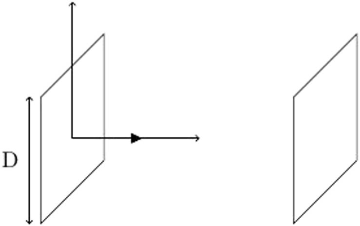
Model of square piezoceramic elements. The distance between two mid-plane of transducers is
The Newton second law in mechanic and third law of Maxwell (electric Guess law) in electromagnetic for charge free medium are expressed, respectively, as follows:
where
Thus,
Note that the matrices are symmetrical, and therefore, values for index 32 are the same as 23 and that for 13 are the same as 31. So we obtain:
According to equation of (1e). For the strain tensor, we introduce
In th following analysis for simplicity, we dropped the superscript of
2.2 Displacement and electric potential of transmitter
Here, the AC voltage is applied to the electrodes of the piezoceramic disk. We will derive the acceleration of the vibrating disk and relate the pressure at the receiver transducer to this acceleration (in the next section).
The nonvanishing strain and electric field components are as follows:
where the time-harmonic factor has been dropped and the comma means derivative with respect to displacement. If we assume sinusoidal function for
By substituting equation (2b) into equation (1c), we obtain:
Equation (2d) can be integrated to yield:
where
where
where
where
As mentioned earlier, the time harmonic factor is dropped and
2.2.1 Boundary conditions (transmitter, free at both sides)
Here, we assumed that the both sides of transmitter piezoceramic square element is free to touch fluid, i.e., the stress at both sides is zero. The boundary conditions between the piezoceramic transmitter disk and the acoustic environment are as follows:
where
To solve the aforementioned equations, add and also subtract the first two equations from each other. The third equation will remain intact.
Thus, the aforementioned constants are as follows:
By knowing these constants, we can express the boundary conditions in the sound wave equation in terms of the velocity of the piezoceramic solid–fluid interface, which is the topic of the next section. The acoustic strength of the transmitter transducer normalized to acoustic volume velocity is calculated as follows:
where
where
2.2.2 Boundary conditions (transmitter, free at front side and fixed at back side)
Here, we assumed that the right sides of transmitter in direction of receiver, piezoceramic square element is free to touch fluid, i.e., the stress at right side is zero; however, the left side is fixed (no strain condition) and there is a back layer with suitable thickness at the left side that suppresses the acoustic pressure. The boundary conditions between the piezoceramic transmitter disk and the acoustic environment are as follows:
where
Derive
Thus, the aforementioned constants are as follows:
The normalized acoustic strength of the transmitter transducer is calculated as follows:
Note that
2.3 Resonance frequency of transmitter
We can consider thickness as a constant and sweep the acoustic strength vs frequency to find the resonance, and in this case, we use analytical approach as a verification method for the optimum frequency we fined from graphical method, i.e., sweeping. In this approach, we find the extremum (minimum in this case) of the average Lagrangian with respect to frequency.
2.3.1 Potential energy
The strain energy per unit volume stored in the piezoceramic due to deformation is expressed as follows:
where
where
These integrals easily can be solved by changing the variable, assume
After substitution of these integral solutions into
It should be noted that we had dropped the sinusoidal term in stress and strain, but we should consider it for calculating the average value of potential energy. We have
2.3.2 Kinetic energy
In contrast to potential energy, which is internal to the system, the kinetic energy is due to a external agent, for obtaining this energy, the newton second law for the transmitter should be solved. Here, we just use the result of section efficiency (section 5). According to this (efficiency) section, velocity is:
Similarly, the average value of kinetic energy is as follows:
2.3.3 External force work as a potential
The mechanical work done on transmitter piezoceramic is caused by piezoelectric force
Note that
2.3.4 Resonance frequency
We will find optimum excitation frequency and thickness at constant excitation voltage. For doing this, we should first take the average of the Lagrangian.
where
As mentioned earlier, the analytical method can be used as a verification of the frequency derived from sweeping the acoustic strength (at given thickness). By solving the aforementioned nonlinear equations numerically in MATLAB, we can find the optimum resonance frequency and even optimum thickness at which we have maximum pressure at a receiver side.
3 Propagation of acoustic waves between transducers
The most exact simplified sound wave equation in viscous fluid without considering compressibility, which can be considered as a model of human body tissue can be described as follows[2] (Kino 1987):
where
Note that the dimension of
By knowing the velocity potential, one can derive the pressure according to the following differential equation (Kino 1987):
Assume a one-dimensional model[3]. We assume the response of equation (11a) as follows:
where
where the bar-sign means frequency domain. By substituting equation (11c) or (11d) into homogenized equation (11a) and drop time harmonic real part terms, we obtain:
Note that we drop the exponential terms.
where
Note that
And the phasor form is:
Thus, the homogeneous plus nonhomogeneous solution in the frequency domain becomes as follows:
By applying boundary condition, we obtain
where we introduced
where
where
where
Note that the dominance of each term in the aforementioned function determines near-field or far-field pressure in acoustic domain. By solving the aforementioned equations, we obtain:
Note that for free-fixed boundary conditions, we should use
where
3.1 Reynolds number
We can define Reynolds number as follows:
This can be interpreted as inertia force (acceleration) to viscous force (friction). Note that it is a nondimensional number. If this term became small, then the pressure decreases substantially with distance from transmitter and the decaying term became dominant with respect to steady terms in pressure function. We will calculate this number in the numerical example section.
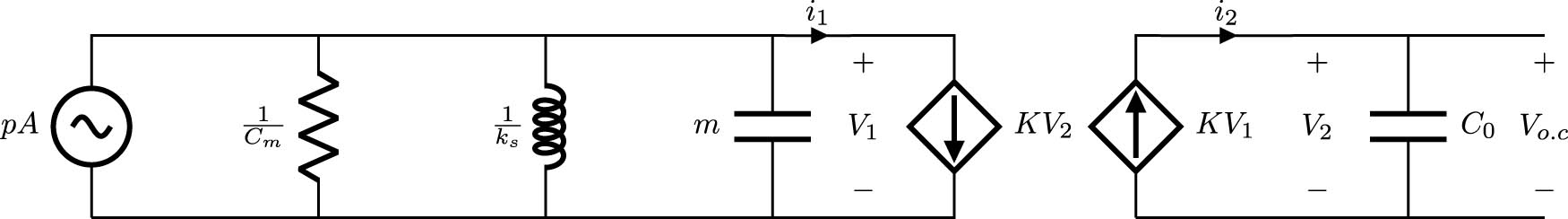
4 Receiver transducer
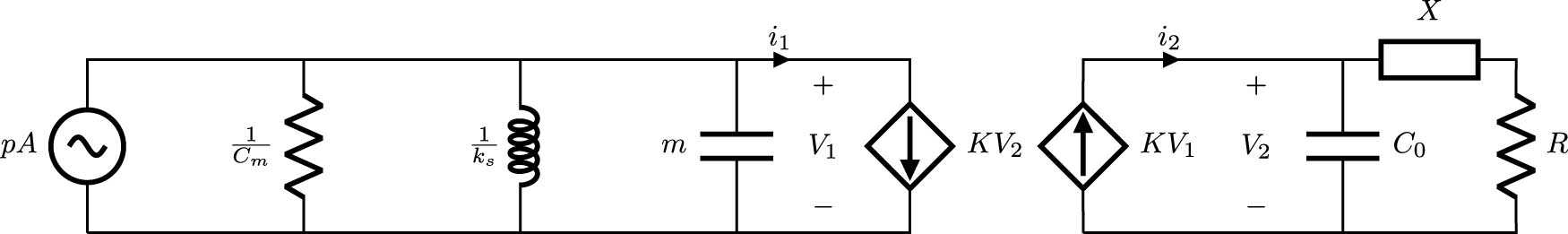
In this section, we express the mechanical and electrical differential equations for resistive, capacitive, and inductive loads and decouple them in the frequency domain so that the electrical damping and output power can be calculated. Figure 2 depicts the general circuit of the equivalent electrical part of the receiver transducer, where

The equivalent electrical part of receiver transducer.
4.1 Resistive load
The second Newton law on the mechanical side and the Kirchhoff current law on the electrical side with
Note that
where the bar sign means frequency domain. And
Therefore, the transfer function is given as follows:
Now we calculate the input electrical power into the electrical domain. Note that only the work of piezoelectric force, i.e.,
After simplifying and transforming the aforementioned equation into standard form, we obtain:
where RMS stands for the root mean square. Note that the
And the resonance condition in which we can calculate the resonance frequency of the receiver transducer from is given as follows:
It is worth noting that this condition guarantees that the mechanical displacement amplitude is maximum, and the frequency that derived from it is also called natural frequency of the receiver piezoceramic element. The active electrical power in the resistor is given as follows:
By applying the resonance condition
And, finally, plugging (24) into (23), the following is obtained
It should be observed that
This condition states that, at resonance, input electrical power in the electrical domain is maximized, i.e., maximum peak when the electrical damping coefficient equals the mechanical damping coefficient.
4.2 Capacitive load
When the load reactance in Figure 2 has a negative value (capacitive load), an analysis approach similar to those for resistive load can be used, which yields to the following equations:
where
4.3 Inductive load
The analysis can be done in the case of an inductive load. The electrical side equations are given as follows:
which, in the frequency domain, becomes
The load voltage in the frequency domain is given as follows:
So, the transfer function is
On the basis of the real and imaginary parts of the transfer function denumerator, we obtain
and, finally, according to (31), the output power is
5 Efficiency
In this section, we derive a formula for efficiency of transmitter and receiver. However, before that, we should define efficiency as output electrical power to input power due to deformation. In other words, we can define efficiency just for direct piezoelectric effect (energy harvesting effect) and not indirect effect. Whenever we have indirect effect such as in transmitter, we should reverse the result and define the efficiency as input electric power to output mechanical power due to velocity and deformation. Otherwise it is value became larger than one.
5.1 Transmitter
The differential equation governing the vibration of transmitter transducer is as follows:
where
Now consider the electrical peak input power to transmitter:
Note that the minus sign in power equation is due to the reverse direction of current into transmitter. After substitution, we have
After simplification, we have
The RMS input value of the power is given as follows:
For deriving the output power of transmitter, it should be noted that the electrical input power to transmitter is converted to mechanical one. In other words, the electrical input power causes the transmitter piezoceramic to have displacement and velocity. Thus, we first should calculate the sum of potential and kinetic energy function (the total energy) with respect to time and take a derivative of it and at the end take the
After simplification and some algebraic manipulation:
Now we can take the derivative of equation (37k) to find the output power of the transmitter transducer.
By taking the RMS of equation (37l), we have:
where
The efficiency is:
Note that according to the definition of efficiency for indirect piezoelectric effect we should reverse the the ratio of output mechanical power to the input electrical power for transmitter transducer.
5.2 Receiver
We define the efficiency for receiver transducer as the ratio of the output power in load resistor to the input power deliver by pressure imposed on transducer by ultrasonic waves. It should be noted that the input power to the receiver energy harvester is equal to the power consumed in the mechanical and electrical dampers (refer to similar article about efficiency from the first author (Dezhara 2023)). We have calculated the electrical damping coefficient for each load and also output power. Thus, we define the efficiency in this case as follows:
where
In this simple case (resistive load), the maximum efficiency for receiver energy harvester can be easily derived:
We conclude that for resistive load, the maximum efficiency of receiver transducer occurs when the load resistance is equal to internal impedance (reactance) of piezoceramic transducer. Note that this resistance is not the optimum resistance for maximum power because generally for energy harvesters, maximum efficiency does not occurs at load that maximize power (Dezhara 2023). The maximum efficiency is obtained by substitution of (38e) into efficiency formula:
6 Design method
Here, we introduce an example to find excitation frequency at constant excitation voltage and thickness by designing maximum acoustic strength parameter to produce maximum pressure at receiver side. It should be noted that both of pressure and acoustic strength peak at same frequencies. The resonance frequency is defined as a frequency that the pressure has a maximum peak at receiver side. Note that the output power depends on area of the transducer, and the more the area, the more the power at constant pressure we have. The pressure varies with time through sinusoidal function; however, for receiver, the phase difference between pressure (excitation force) and load voltage (i.e., Kv which is piezoelectric force) is always
6.1 Numerical example
Let us assume to know the mechanical damping coefficient, as well as the piezoelectric coupling factor between the mechanical and electrical side of receiver transducer and also mass of the transducer[6]. Furthermore, assume other parameters for a commercial piezoceramic transducer and the acoustic environment as listed in Tables 1, 2, and 3.
Material properties of PIC155 and geometric constants
| Symbol | Parameter | Value | Unit |
|---|---|---|---|
|
|
Density | 7,800 |
|
|
|
Relative permittivity | 1,450 | — |
|
|
Elastic constant |
|
|
| Coupling factor |
|
0.69 | — |
| Distance | L | 5 | cm |
| Square length | D | 1.46 | cm |
| Half of the thickness | h |
|
mm |
| Peak excitation voltage |
|
10 | V |
| Coupling factor | K | 2.16 |
|
Properties of acoustic environment (distilled water at
| Symbol | Parameter | Value | Unit (SI) |
|---|---|---|---|
|
|
Sound velocity | 1,498 |
|
|
|
Bulk viscosity |
|
Pa s |
|
|
Shear viscosity |
|
Pa s |
|
|
Density of fluid | 997 |
|
Mechanical parameters of transducers
| Symbol | Parameter | Value | Unit (SI) |
|---|---|---|---|
|
|
Mass (2.1 mm thickness) | 3.49 | g |
|
|
Mechanical stiffness (2.1 mm thickness) | 259,893,847 |
|
|
|
Mechanical damping | 0.31 |
|
Note that the value of
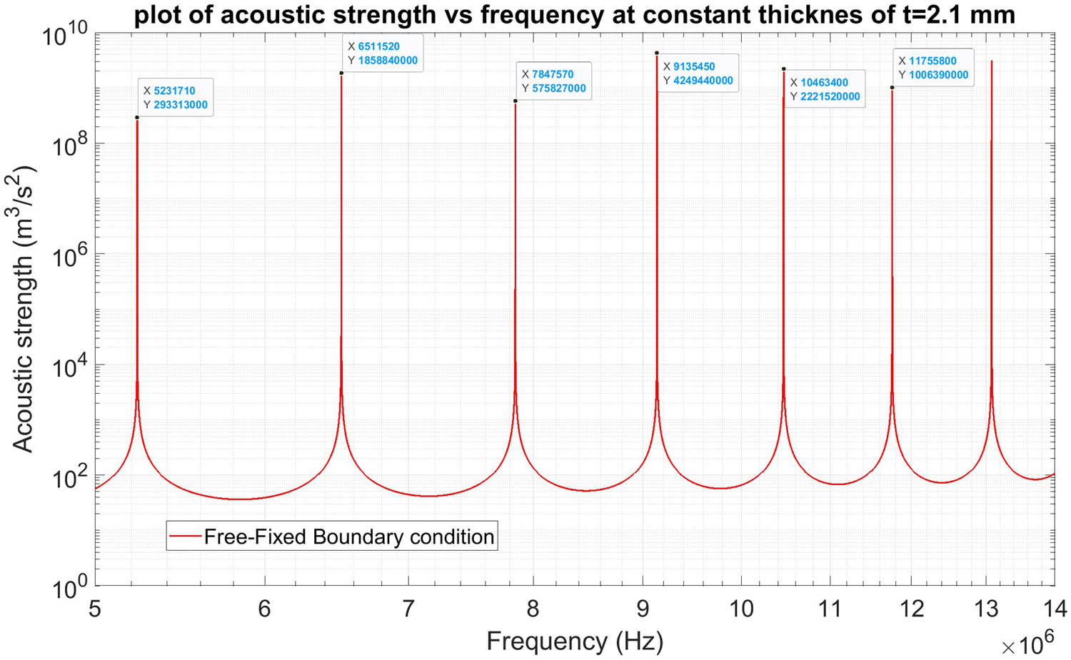
Plot of acoustic strength vs frequency.

Plot of pressure vs frequency at constant distance between transducers, the resonance frequency is 9.13545 MHz,

Plot of output power vs resistive load for free-fixed boundary condition.

Plot of output power vs capacitive load for free-fixed boundary condition.

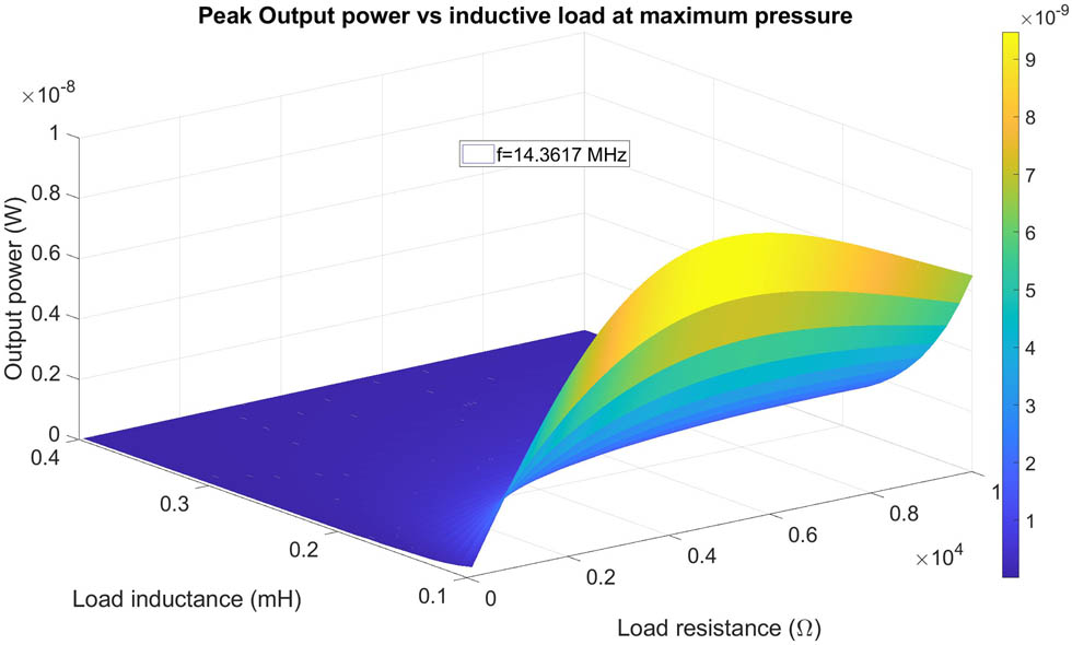
Plot of output power vs inductive load for free-fixed boundary condition.
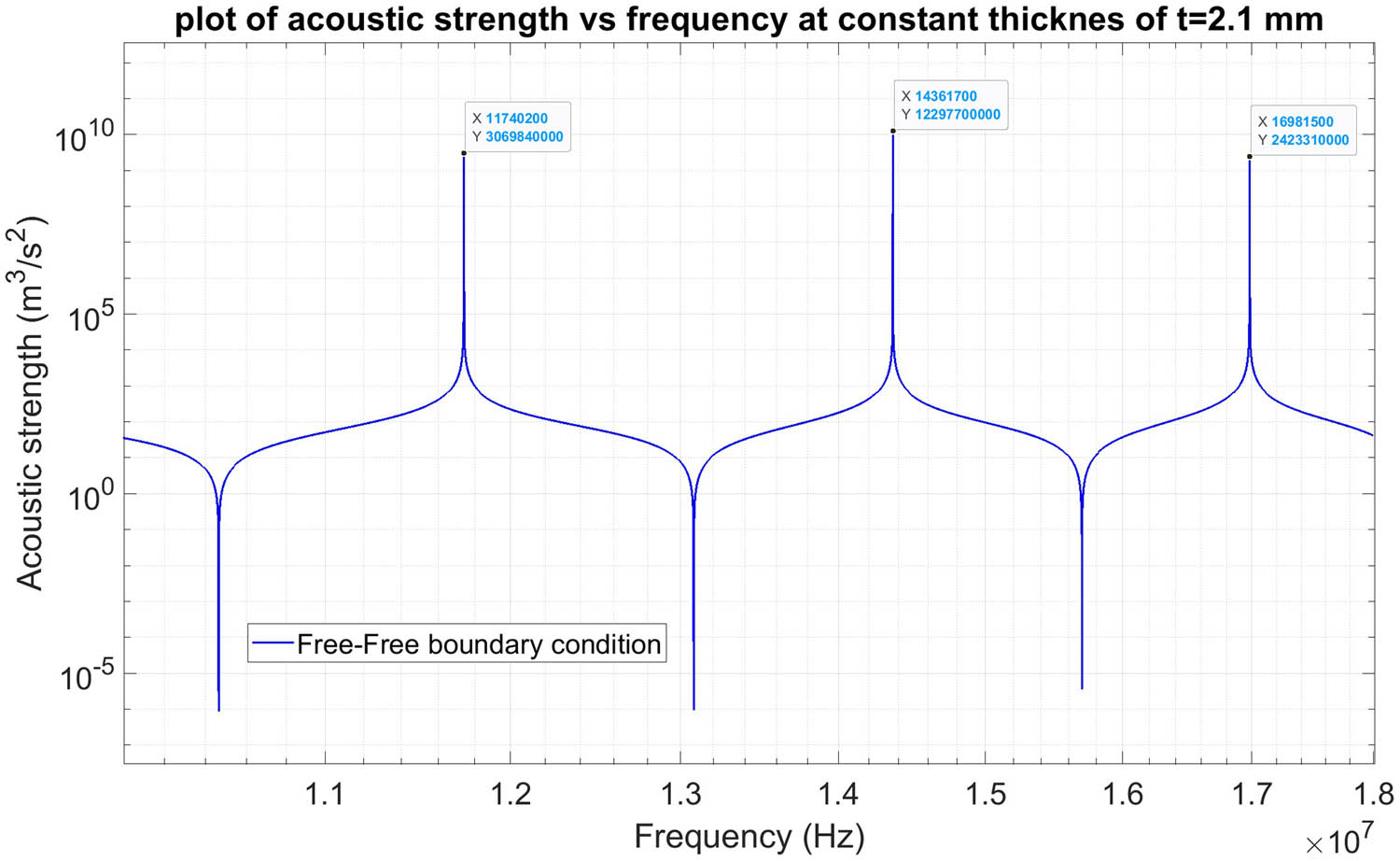
Plot of acoustic strength vs frequency.

Plot of pressure vs frequency at constant distance between transducers, the resonance frequency is 11.7402 MHz, L = 5 cm.

Plot of output power vs resistive load for free-free boundary condition.
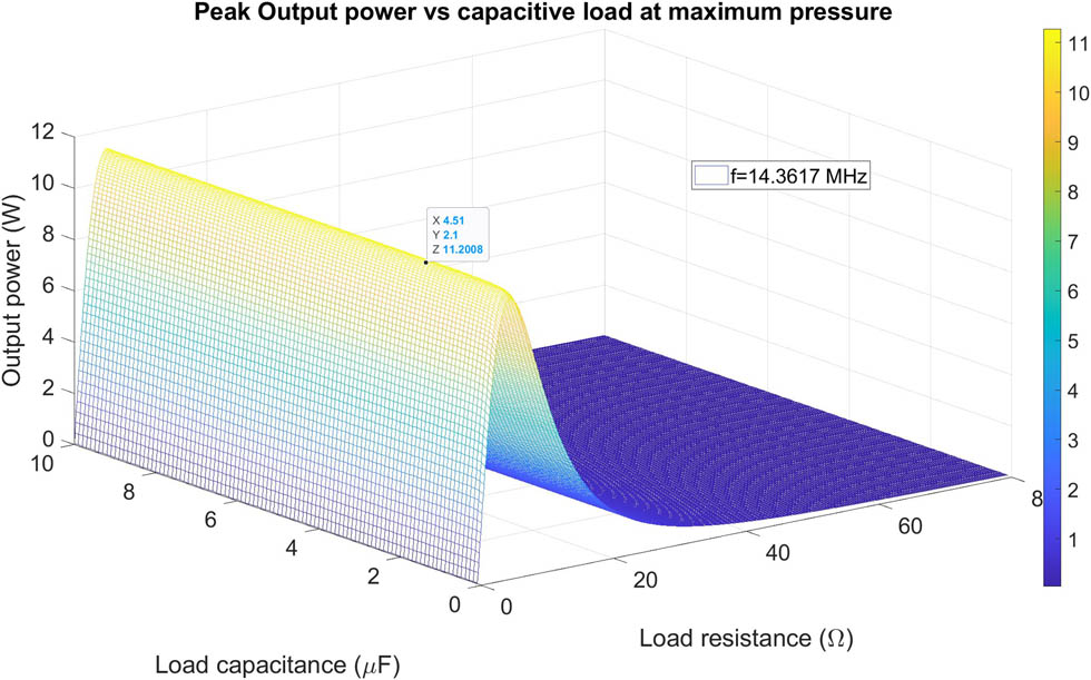
Plot of output power vs capacitive load for free-free boundary condition.
Plot of output power vs inductive load for free-free boundary condition.
We also include the mechanical parameters (Table 3) such as the stiffness of the transducers, which have importance in our calculations. It should be noted that the value of stiffness is calculated using a structural model in MATLAB.
According to Figure 13, we can calculate the stiffness (the ratio of force due to pressure over displacement), as
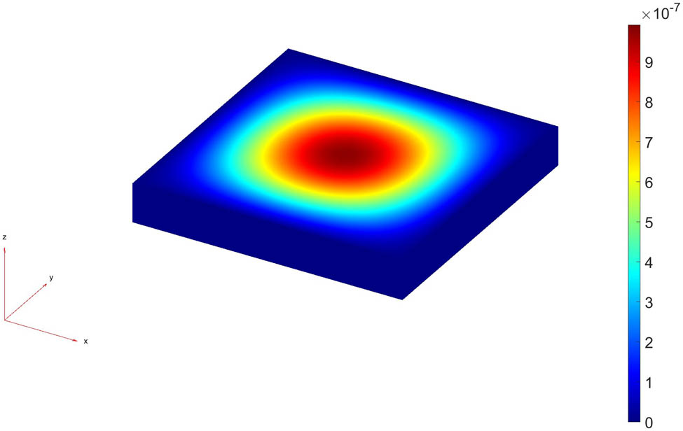
Deflection of receiver transducer (with 2.1 mm thickness) due to imposed pressure of 1.19448 MPa on it vs displacement (in meter) by finite element method in MATLAB.
6.1.1 Calculation of efficiency
Note that the maximum efficiency for resistive load based on equation (38f) and for free-fixed transmitter (Table 4) radiation (
Transmitter efficiency (free-fixed boundary conditions)
| Parameter | Value |
|---|---|
|
|
0.5748 mW |
|
|
|
|
|
|
Receiver efficiency (free-fixed boundary conditions)
| Resistive load | Capacitive load | Inductive load |
|---|---|---|
|
|
|
|
| — |
|
|
|
|
|
|
Transmitter efficiency (free-free boundary conditions)
| Parameter | Value |
|---|---|
|
|
0.8235 mW |
|
|
|
|
|
|
Receiver efficiency (free-free boundary conditions)
| Resistive load | Capacitive load | Inductive load |
|---|---|---|
|
|
|
|
| — |
|
|
|
|
|
|
6.1.2 Calculation of resonance frequency
Here, we plot the average Lagrangian for free-fixed boundary condition, and as seen from the plot, it has a minimum at frequency of 9.13545 MHz at constant thickness of 2.1 mm. The reveres is also true, i.e., it also has minimum at thickness of 2.1 mm and constant frequency of 9.13545 MHz (Figures 14 and 15).
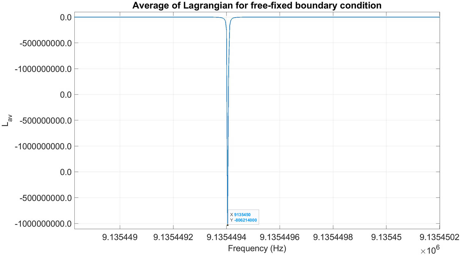
Extremum (minimum) of the Lagrangian with respect to frequency at thickness of

Extremum (minimum) of the Lagrangian with respect to thickness at frequency of
The Reynolds number for free-fixed boundary conditions is:
7 Discussion
From the plot of acoustic strength vs thickness (Figure 3), we see that the fixed-free boundary condition leads to multi-resonance at different acoustic strengths. On the other hand, the free-free boundary condition leads to resonance and antiresonance. Now a question may arises here is that where these two different behaviors come from?. The answer to this curiosity is that the behavior of transmitter under the free-free boundary condition is due to constructive and destructive interference. These interferences stems from forward and backward traveling wave from transmitter which causes constructive interference and resonance and destructive interference and antiresonance. However, the transmitter behavior under free-fixed boundary condition experience just radiation of forward traveling acoustic wave and its backward radiation suppressed by a layer with suitable thickness and that is why we do not see any antiresonance under this boundary condition. From mechanical design point of view, we should ask ourselves that does the pressure at resonance frequency cause mechanical failure in receiver transducer?. If you multiply the pressure by area of the receiver transducer, it leads to a large force in the order of several hundreds kilograms on small area of receiver especially for the case of free-free boundary conditions. Calculation of stress and strain due to this force is beyond the topic and scope of our article; however, we are free to choose a less excitation frequency and as a result less pressure peak for the safety reasons.
8 Conclusion
We conclude that by the resistive load, we can extract more power with even better efficiency with compared to capacitive and inductive loads. We also conclude that in the case of free-fixed boundary conditions in addition to graphical method, the resonance frequency can be calculated by energy methods, i.e., Lagrangian.
-
Funding information: None declared.
-
Author contributions: Conceptualization, Alfio Dario Grasso and Aboozar Dezhara; methodology, Aboozar Dezhara; data curation, Aboozar Dezhara and Andrea Ballo; writing – original draft preparation, Aboozar Dezhara; writing – review and editing, Aboozar Dezhara and Alfio Dario Grasso; visualization, Aboozar Dezhara; supervision, Alfio Dario Grasso and Andrea Ballo. All authors have accepted responsibility for the entire content of the manuscript and agreed to the published version.
-
Conflict of interest: The authors declare no conflicts of interest regarding this article.
-
Data availability statement: Reported data in this manuscript are available upon request to the corresponding author.
Appendixes
Here, we consider impedance matching for the receiver side and also deriving some parameters analytically.
A.1 Impedance matching (receiver side)
The mobility similarity, rather than the impedance similarity, of spring-mass system with electrical circuits as according to Dezhara (2022), Beeby et al. (2006), Ottman et al. (2002), Priya et al. (2017) is used in this article.
Figure A1 depicts the equivalent circuit of the PZT at the receiver side. The term
Receiver side transducer circuit.
Open circuit voltage.
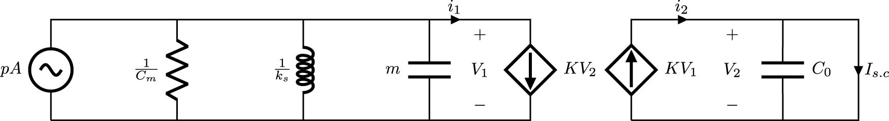
Short circuit current.
In regarding to Figure A3, we have:
where
Note that the optimum resistance and reactance does not depend on the pressure imposed on receiver transducer.
A.2 Mechanical damping coefficient and short circuit piezoelectric element
The mechanical damping coefficient can be calculated from logarithmic reduction law by measuring the consecutive peaks of transient response of piezoelectric shorted circuit in a oscilloscope.
To calculate the value of
If you solve the differential equation (A7), we have:
we assumed that we have under damped oscillation, i.e.,
If you equate the relations of (A6e) and (A9), we can calculate the values of
Thus, we obtain:
Note that the velocity is also decayed as
A.3 Piezoelectric Coupling Factor
Here, we propose two methods for deriving a formula for calculating the value of the coupling factor between the mechanical and electrical sides of piezoceramic transducers.
A.3.1 Method 1 (analytical method)
The value of
By substituting (A12d) into (A12a), we have:
By solving the aforementioned differential equation and obtaining the nonhomogeneous and homogeneous solution, we have:
where
where
From equation (A12i), we can write guess law as follows:
After substituting relation of (A12k) into (26), we can find strain along the (33) direction.
By knowing the the value of strain, we can find stress in (33) direction from equation (A12h).
Now we should relate the stress force to piezoelectric force (
From equation (A12o), we can find a formula for
If we calculate the value of
A.3.2 Method 2 (experimental method)
In the second method, we use equation (A2f). Note that everything is known except the parameter
We can put the aforementioned equation in the following form:
By solving the aforementioned equation symbolically in MATLAB, we can find the acceptable values of
References
Beeby S. P., Tudor M. J., and White N. M. (2006). “Energy harvesting vibration sources for microsystems applications,” Measurement Science and Technology, vol. 17, no. 12, R175. 10.1088/0957-0233/17/12/R01Search in Google Scholar
Chen N., Wei T., Ha D. S., Jung H. J., and Lee S. (2018). “Alternating resistive impedance matching for an impact-type microwind piezoelectric energy harvester,” IEEE Transactions on Industrial Electronics, vol. 65, no. 9, pp. 7374–7382. 10.1109/TIE.2018.2793269Search in Google Scholar
Dezhara A. (2022). “Frequency response locking of electromagnetic vibration-based energy harvesters using a switch with tuned duty cycle,” Energy Harvesting and Systems, vol. 9, no. 1, pp. 83–96. 10.1515/ehs-2021-0057Search in Google Scholar
Dezhara A. (2023). “The efficiency of linear electromagnetic vibration-based energy harvester at resistive, capacitive and inductive loads,” Energy Harvesting and Systems, vol. 10, no. 1, pp. 93–104. 10.1515/ehs-2022-0028Search in Google Scholar
Dezhara A. (2024). “Non-transient optimum design of nonlinear electromagnetic vibration-based energy harvester using homotopy perturbation method,” Energy Harvesting and Systems, vol. 11, no. 1, p. 20220101. 10.1515/ehs-2022-0101Search in Google Scholar
Erturk A. and Inman D. J. (2008). “Issues in mathematical modeling of piezoelectric energy harvesters,” Smart Materials and Structures, vol. 17, no. 6, pp. 065016. 10.1088/0964-1726/17/6/065016Search in Google Scholar
Humphrey V. F. (2007). “Ultrasound and matter-physical interactions,” Progress in Biophysics and Molecular Biology, vol. 93, no. 1, pp. 195–211. Effects of ultrasound and infrasound relevant to human health. 10.1016/j.pbiomolbio.2006.07.024Search in Google Scholar PubMed
Jiang L., Yang Y., Chen Y., and Zhou Q. (2020). “Ultrasound-induced wireless energy harvesting: From materials strategies to functional applications,” Nano Energy, vol. 77, p. 105131. 10.1016/j.nanoen.2020.105131Search in Google Scholar PubMed PubMed Central
Kim H., Priya S., Stephanou H., and Uchino K. (2007). “Consideration of impedance matching techniques for efficient piezoelectric energy harvesting,” IEEE Transactions on Ultrasonics, Ferroelectrics, and Frequency Control, vol. 54, no. 9, pp. 1851–1859. 10.1109/TUFFC.2007.469Search in Google Scholar PubMed
Kino G. S. (January 1, 1987). Acoustic waves: Devices, imaging, and analog signal processing, Prentice Hall. Search in Google Scholar
Liang J. and Liao W.-H. (2012). “Impedance modeling and analysis for piezoelectric energy harvesting systems,” IEEE/ASME Transactions on Mechatronics, vol. 17, no. 6, pp. 1145–1157. 10.1109/TMECH.2011.2160275Search in Google Scholar
Lin J. (2006). “A new ieee standard for safety levels with respect to human exposure to radio-frequency radiation,” IEEE Antennas and Propagation Magazine, vol. 48, no. 1, pp. 157–159. 10.1109/MAP.2006.1645601Search in Google Scholar
Ottman G., Hofmann H., Bhatt A., and Lesieutre G. (2002). “Adaptive piezoelectric energy harvesting circuit for wireless remote power supply,” IEEE Transactions on Power Electronics, vol. 17, no. 5, pp. 669–676. 10.1109/TPEL.2002.802194Search in Google Scholar
Ozeri S. and Shmilovitz D. (2010). “Ultrasonic transcutaneous energy transfer for powering implanted devices,” Ultrasonics, vol. 50, no. 6, pp. 556–566. Search in Google Scholar
Ozeri S. and Shmilovitz D. (2010 May). “Ultrasonic transcutaneous energy transfer for powering implanted devices,” Ultrasonics, vol. 50, no. 6, pp. 556–66. 10.1016/j.ultras.2009.11.004Search in Google Scholar PubMed
Piech D. K., Johnson B. C., Shen K., Ghanbari M. M., Li K. Y., Neely R. M., et al. (2020). “A wireless millimetre-scale implantable neural stimulator with ultrasonically powered bidirectional communication,” Nature Biomedical Engineering, vol. 4, pp. 207–222. 10.1038/s41551-020-0518-9Search in Google Scholar PubMed
Pritchard W. F., and Carey R. F. (1997). “Food and drug administration and regulation of medical devices in radiology,” Radiology, vol. 205, no. 1, pp. 27–36. 10.1148/radiology.205.1.9314955Search in Google Scholar PubMed
Priya S., Song H.-C., Zhou Y., Varghese R., Chopra A., Kim S.-G., et al. (2017). “A review on piezoelectric energy harvesting: Materials, methods, and circuits,” Energy Harvesting and Systems, vol. 4, no. 1, pp. 3–39. 10.1515/ehs-2016-0028Search in Google Scholar
Roes M. G. L., Duarte J. L., Hendrix M. A. M., and Lomonova E. A. (2013). “Acoustic energy transfer: A review,” IEEE Transactions on Industrial Electronics, vol. 60, no. 1, pp. 242–248. 10.1109/TIE.2012.2202362Search in Google Scholar
Safaei M., Sodano H. A., and Anton S. R. (2019). “A review of energy harvesting using piezoelectric materials: state-of-the-art a decade later (2008-2018),” Smart Materials and Structures, vol. 28, no. 11, pp. 113001. 10.1088/1361-665X/ab36e4Search in Google Scholar
Shahab S. (2014). “Contactless ultrasonic energy transfer: Acoustic-piezoelectric structure interaction modeling and performance enhancement,” Smart Materials and Structures, vol. 23, pp. 125032. 10.1088/0964-1726/23/12/125032Search in Google Scholar
Sherrit S. (2008). “The physical acoustics of energy harvesting,” Proceedings - IEEE Ultrasonics Symposium. 10.1109/ULTSYM.2008.0253Search in Google Scholar
Taalla R. V., Arefin M. S., Kaynak A., and Kouzani A. Z. (2019). “A review on miniaturized ultrasonic wireless power transfer to implantable medical devices,” IEEE Access, vol. 7, pp. 2092–2106. 10.1109/ACCESS.2018.2886780Search in Google Scholar
Tseng V. F.-G., Bedair S. S., Radice J. J., Drummond T. E., and Lazarus N. (2020). “Ultrasonic lamb waves for wireless power transfer,” IEEE Transactions on Ultrasonics, Ferroelectrics, and Frequency Control, vol. 67, no. 3, pp. 664–670. 10.1109/TUFFC.2019.2949467Search in Google Scholar PubMed
Wang H., Shan X., Xie T., and Fang M. (2011). “Analyses of impedance matching for piezoelectric energy harvester with a resistive circuit,” In: Proceedings of 2011 International Conference on Electronic & Mechanical Engineering and Information Technology, vol. 4, pp. 1679–1683. 10.1109/EMEIT.2011.6023423Search in Google Scholar
Wang J., Chen Z., Li Z., Jiang J., Liang J., and Zeng X. (2022). “Piezoelectric energy harvesters: An overview on design strategies and topologies,” IEEE Transactions on Circuits and Systems II: Express Briefs, vol. 69, no. 7, pp. 3057–3063. 10.1109/TCSII.2022.3173966Search in Google Scholar
Wang X., Song J., Liu J., Wang Z. L. (2007 Apr 6). “Direct-current nanogenerator driven by ultrasonic waves,” Science, vol. 316, no. 5821, pp. 102–5. 10.1126/science.1139366Search in Google Scholar PubMed
Wu M., Chen X., Qi C., and Mu X. (2020). “Considering losses to enhance circuit model accuracy of ultrasonic wireless power transfer system,” IEEE Transactions on Industrial Electronics, vol. 67, no. 10, pp. 8788–8798. 10.1109/TIE.2019.2947802Search in Google Scholar
Yang Z., Zeng D., Wang H., Zhao C., and Tan J. (2015). “Harvesting ultrasonic energy using 1-3 piezoelectric composites,” Smart Materials and Structures, vol. 24, no. 7, pp. 075029. 10.1088/0964-1726/24/7/075029Search in Google Scholar
Yang Z., Zeng D., Zhao C., Li F., and Wang H. (2013). “Wireless energy transmission using ultrasound for implantable devices,” In 2013 Symposium on Piezoelectricity, Acoustic Waves, and Device Applications (pp. 1–4). IEEE. 10.1109/SPAWDA.2013.6841073Search in Google Scholar
© 2024 the author(s), published by De Gruyter
This work is licensed under the Creative Commons Attribution 4.0 International License.
Articles in the same Issue
- Solar photovoltaic-integrated energy storage system with a power electronic interface for operating a brushless DC drive-coupled agricultural load
- Analysis of 1-year energy data of a 5 kW and a 122 kW rooftop photovoltaic installation in Dhaka
- Reviews
- Real yields and PVSYST simulations: comparative analysis based on four photovoltaic installations at Ibn Tofail University
- A comprehensive approach of evolving electric vehicles (EVs) to attribute “green self-generation” – a review
- Exploring the piezoelectric porous polymers for energy harvesting: a review
- A strategic review: the role of commercially available tools for planning, modelling, optimization, and performance measurement of photovoltaic systems
- Comparative assessment of high gain boost converters for renewable energy sources and electrical vehicle applications
- A review of green hydrogen production based on solar energy; techniques and methods
- A review of green hydrogen production by renewable resources
- A review of hydrogen production from bio-energy, technologies and assessments
- A systematic review of recent developments in IoT-based demand side management for PV power generation
- Research Articles
- Hybrid optimization strategy for water cooling system: enhancement of photovoltaic panels performance
- Solar energy harvesting-based built-in backpack charger
- A power source for E-devices based on green energy
- Theoretical and experimental investigation of electricity generation through footstep tiles
- Experimental investigations on heat transfer enhancement in a double pipe heat exchanger using hybrid nanofluids
- Comparative energy and exergy analysis of a CPV/T system based on linear Fresnel reflectors
- Investigating the effect of green composite back sheet materials on solar panel output voltage harvesting for better sustainable energy performance
- Electrical and thermal modeling of battery cell grouping for analyzing battery pack efficiency and temperature
- Intelligent techno-economical optimization with demand side management in microgrid using improved sandpiper optimization algorithm
- Investigation of KAPTON–PDMS triboelectric nanogenerator considering the edge-effect capacitor
- Design of a novel hybrid soft computing model for passive components selection in multiple load Zeta converter topologies of solar PV energy system
- A novel mechatronic absorber of vibration energy in the chimney
- An IoT-based intelligent smart energy monitoring system for solar PV power generation
- Large-scale green hydrogen production using alkaline water electrolysis based on seasonal solar radiation
- Evaluation of performances in DI Diesel engine with different split injection timings
- Optimized power flow management based on Harris Hawks optimization for an islanded DC microgrid
- Experimental investigation of heat transfer characteristics for a shell and tube heat exchanger
- Fuzzy induced controller for optimal power quality improvement with PVA connected UPQC
- Impact of using a predictive neural network of multi-term zenith angle function on energy management of solar-harvesting sensor nodes
- An analytical study of wireless power transmission system with metamaterials
- Hydrogen energy horizon: balancing opportunities and challenges
- Development of renewable energy-based power system for the irrigation support: case studies
- Maximum power point tracking techniques using improved incremental conductance and particle swarm optimizer for solar power generation systems
- Experimental and numerical study on energy harvesting performance thermoelectric generator applied to a screw compressor
- Study on the effectiveness of a solar cell with a holographic concentrator
- Non-transient optimum design of nonlinear electromagnetic vibration-based energy harvester using homotopy perturbation method
- Industrial gas turbine performance prediction and improvement – a case study
- An electric-field high energy harvester from medium or high voltage power line with parallel line
- FPGA based telecommand system for balloon-borne scientific payloads
- Improved design of advanced controller for a step up converter used in photovoltaic system
- Techno-economic assessment of battery storage with photovoltaics for maximum self-consumption
- Analysis of 1-year energy data of a 5 kW and a 122 kW rooftop photovoltaic installation in Dhaka
- Shading impact on the electricity generated by a photovoltaic installation using “Solar Shadow-Mask”
- Investigations on the performance of bottle blade overshot water wheel in very low head resources for pico hydropower
- Solar photovoltaic-integrated energy storage system with a power electronic interface for operating a brushless DC drive-coupled agricultural load
- Numerical investigation of smart material-based structures for vibration energy-harvesting applications
- A system-level study of indoor light energy harvesting integrating commercially available power management circuitry
- Enhancing the wireless power transfer system performance and output voltage of electric scooters
- Harvesting energy from a soldier's gait using the piezoelectric effect
- Study of technical means for heat generation, its application, flow control, and conversion of other types of energy into thermal energy
- Theoretical analysis of piezoceramic ultrasonic energy harvester applicable in biomedical implanted devices
- Corrigendum
- Corrigendum to: A numerical investigation of optimum angles for solar energy receivers in the eastern part of Algeria
- Special Issue: Recent Trends in Renewable Energy Conversion and Storage Materials for Hybrid Transportation Systems
- Typical fault prediction method for wind turbines based on an improved stacked autoencoder network
- Power data integrity verification method based on chameleon authentication tree algorithm and missing tendency value
- Fault diagnosis of automobile drive based on a novel deep neural network
- Research on the development and intelligent application of power environmental protection platform based on big data
- Diffusion induced thermal effect and stress in layered Li(Ni0.6Mn0.2Co0.2)O2 cathode materials for button lithium-ion battery electrode plates
- Improving power plant technology to increase energy efficiency of autonomous consumers using geothermal sources
- Energy-saving analysis of desalination equipment based on a machine-learning sequence modeling