Impact of using a predictive neural network of multi-term zenith angle function on energy management of solar-harvesting sensor nodes
-
Murad Al-Omary

 ,
Rafat Aljarrah
,
Aiman Albatayneh
,
Dua’a Alshabi
and
Khaled Alzaareer
,
Rafat Aljarrah
,
Aiman Albatayneh
,
Dua’a Alshabi
and
Khaled Alzaareer

Abstract
Using the Neural Networks to predict solar harvestable energy would contribute to prolonging the duration of the effective operation and thus less consumption in solar-harvesting sensor nodes. The NNs with higher prediction accuracy have the longest effective operation. Till now, the NNs that use the zenith angle function as input have been utilized with only two terms. This paper shows the advantages of using a multi-term zenith angle function on the energy management in the nodes. To this end, this paper considers two, three, and four terms for the function of the zenith angle. The results showed that the case of four terms has the lowest prediction mistakes on average (0.83%) compared to (2.13% and 1.75%) for the cases of two and three terms, respectively. This is followed by a reduction in energy consumption in favor of four terms case. For one month simulation period with hourly prediction, the sensor node worked at the higher consumption mode (M2) in the case of four terms 4 hours less than three terms and 7 hours less than two terms case. Thus, increasing the number of terms in the zenith angle function leads to higher accuracy and less energy consumption.
1 Introduction
Wireless Sensor Network (WSN) consists of plenty of tiny sensing devices. The main functionality of these devices is to monitor and record the physical or environmental variables directly (e.g., temperature, sound, light, pressure, distance and humidity) (Carlos-Mancilla, López-Mellado, Siller 2016; Galar and Kumar 2017; Senouci and Mellouk 2016). The sensed data is forwarded wirelessly to a base station, where the required computing and processing take place to give the desired results. Such wireless nodes are serviceable in vast domains including but not limiting engineering, medical, industrial, and intelligent agricultural applications (Matin and Islam 2012; Senouci and Mellouk 2016).
Typically, the sensor node can comprise four parts: the powering (storage), the communication (the transceiver), the processing or control (the microcontroller), and the sensing part. All those parts could be represented by block diagrams, as in Figure 1, which is taken from (Xia 2009). For the power storage part, small non-rechargeable/rechargeable batteries with a limited capacity and short lifetime are usually utilized. Due to the proven unfeasibility of recharging and replacing these batteries, new renewable technologies are required to extend the network lifetime leading to sustainable networks (Liang et al. 2019; Munir and Dyo 2018). Economically, these technologies could save the cost of recharging and replacements, especially in rugged and rural regions, where access is abundantly needed and challenging jointly (Zou et al. 2017).

Block diagram for parts of sensor nodes.
Building sensor nodes with reliable operation became a necessary need for the users of the networks. Because of existing renewable energy technologies today besides these sensors, such a target switched to a challenge (Azeem et al. 2019; Xu, Tang, and Xiang 2022). Although powering the sensors through renewable resources has been proposed as a solution to overcome the problem of batteries’ limitations, the energy from the surrounding environment could be provided by variant types like solar, wind, thermal, vibrations, and piezoelectric (Avtar et al. 2019; Prauzek et al. 2018; Sah and Amgoth 2020). However, solar energy is the most preferred form for powering sensor nodes. One of the main reasons for solar being heavily used as a power source is represented by the small size of the module compared to its output energy which can reach up to 15 W/cm2. Notably, the low cost of the solar cell components is also counted in favor of solar form over the others (Li and Shi 2015; Mabon et al. 2019; Sharma et al. 2018).
The first step toward fulfilling sustainable networks is to make the sensor units more practical and efficient. However, this could not happen without a good management plan that ensures balancing between available and consumed energy (Lorincz et al. 2019). Thus, studied management plans have been implemented in the microcontrollers of the nodes (Goyal and Sonal 2016; Silva, Liu, and Moghaddam 2012). Additionally, the management plans require a prediction as a supporting tool aiming to fulfill prior knowledge about the available energy. This prediction, in the role, will contribute to adjusting the sensor node to the necessary operation mode (Jankovic and Saranovac 2020).
Neural networks have been used commonly to predict profiles of harvested energy in sensor nodes. This is denoted by the accurate prediction method compared to the primitive statistical and stochastic ones. Accordingly to the variety of the utilized neural networks, the accuracy of prediction changes leading to a change in the manageability level (Al-Omary et al. 2019). One of the most recent neural networks is the network that was used with sensors and included historical inputs and the zenith angle function of two terms as meteorological inputs (Engmann et al. 2021). About this issue, this paper aims to study the impact of using a predictive neural network of multi-term zenith angle functions on the energy management of sensor nodes supplied with solar energy.
Regarding the structure of this paper, Section 2 handles the previous prediction techniques in solar-harvesting sensor units. In Section 3 of this paper, detailed clarifications about some statistical methods have been presented, specifically; the time series-based ones. In Section 4, the previous predictive neural networks that were used with these nodes are provided. Section 5 comes after that to identify the cases that would be considered for studying the impact of using multi-term zenith angle function with the predictive networks. It also contains a subsection in which the measured correlation coefficients and the associated prediction mistakes for these cases are offered. In the last section, Section 6, the results and the findings of the impact of employing these cases on the management of energy consumption have been announced by comparing the working modes that appeared for a sensor node within a specific simulation period.
2 State of the art
Energy forecasting for solar systems varies from a long-term forecasting scale (year or more) to a short-term forecasting scale ranging from minutes to a few hours. WSN requires short-term predictions for more accuracy. Several methods were used for that purpose, where most of them employ a group of previous energy readings recorded during current and past days considering 1-h duration (Engmann et al. 2021). These methods would be overviewed briefly from the most ancient to the most recent ones in the following paragraphs.
The simplest and oldest method is created by authors in (Kansal et al. 2007) and named Exponentially Weighted Moving Average (EWMA). The predictable energy for a specific time window is assumed here as weights from the energy collected two days before in the corresponding windows. Using this method at sudden fluctuations in the weather leads to large prediction mistakes, which is considered a drawback. The Weather Conditioned Moving Average (WCMA) method in (Piorno et al. 2009), effectively overcomes this drawback by taking into consideration the harvested energy from both current and past days. The latter method performs the prediction by inserting the mean value of similar samples in the past days and a scaling factor called (GAP) to the prediction equation.
Benefiting from the feedback mechanism, the authors in (Bergonzini, Brunelli, and Benini 2010) developed an improved method named WCMA-PDR. This method applies a phase displacement regulator to reduce the prediction mistake in WCMA. In (Jiang et al. 2010), the authors suggested another improved version of WCMA, with higher accuracy and very low overhead, called Weather Conditioned Selective Moving Average (WCSMA). This method classifies the past days into sunny and cloudy categories and then predicts the energy by choosing the most similar window from these categories according to the type of the predictable day.
Two years after (WCSMA), Pro-Energy was proposed by the authors in (Cammarano et al. 2012) as a novel procedure to expect the upcoming solar energy. This procedure extracts the most similar profile in the past days and employs it in addition to the current day’s observations in the prediction equation. During the same year, the authors in (Hassan and Bermak 2012) presented another prediction that offered an additive decomposition, Solar Energy Prediction Additive Decomposition (SEPAD); where both the daily and seasonal terms of the sun were considered.
The aforementioned methods were followed by another contribution for the authors in (Le et al. 2013), who proposed an adaptive filter to forecast energy from the sun. The IPro-Energy technique that is indicated in (Khan, Qureshi, and Iqbal 2015) appeared after that as an improved version of the Pro-Energy method. Then, Markov chains with increasing order were used by a prediction model called Accurate Solar Irradiance Model (ASIM) as proposed in (Ghuman et al. 2015).
The field of predicting solar energy has improved rapidly as many approaches with different structures and parameters were proposed. The workers on another piece of research in (Kosunalp 2016) proposed an updated version of the predicted profile of EWMA by adding the daily ratio as a new parameter to get another prediction technique for energy-harvesting, (QL-SEP). In another research (Edalat and Motani 2016), WCMA was used to derive another prediction model called Autoregressive Weather-Conditioned Moving Average (AR-WCMA). On other hand, the authors in (Zou et al. 2016), added the environmental shadow as an energy prediction parameter. Later on, the Pro-Energy-VLT method in (Cammarano et al. 2016) presented a combination of the Pro-Energy predictor with time windows of variable lengths.
Combining the global knowledge with the local knowledge in the EWMA was the addition found by the authors in (Thakur, Prasad, and Verma 2017). On the other hand, the research in (Dehwah, Elmetennani, and Claudel 2017) gave a universal dynamic version of the WCMA method in which a prediction and evaluation of solar power fluctuations are implemented in sensors, named UD-WCMA. The Real-Forecast Weather Moving Average (RWMA) showed up as a reliable and efficient forecasted technique (Ren et al. 2018). It employed the mistake of the harvested solar energy to adjust the prediction results. In Bouguera et al. (2018), Solar Energy Predictor for Communicating Sensors (SEPCS) was offered. This predictor uses the previous energy recorded readings to expect the availability of solar energy in the coming short term.
Moreover, the authors in (Al-Omary 2019) developed a forecasting neural network with higher accuracy compared to the time series-based methods and neural networks that just use historical inputs. This neural network adds the zenith angle as an additional meteorological parameter to the historical inputs. Another enhancement has been fulfilled by incorporating a tuning factor as well as a fine adjustment index to the Pro-Energy method. The authors of this method which appears in (Deb and Roy 2021) called their method “Enhanced Pro”. Lastly, in (Al-Omary et al. 2021), a recent technique aiming to enhance the prediction of solar energy over one day, by combining the previous two-time series-based approaches (EWMA and WCMA) was presented. Named Exponentially Weighted Weather Condition (EWWC). Finally, the “Ratioed Pro-Energy” predictor has been developed by the authors in (Al-Omary et al. 2022a), as a corrected copy of the Pro-Energy to be beneficial for small-scale solar worked devices including sensor nodes.
3 Time series prediction methods
The most common time series-based methods were presented in this section, with more details about their characteristics and prediction equations. As shown in Table 1, these methods include the Exponentially Weighted Moving Average (EWMA), the Weather Conditioned Moving Average (WCMA) and the Pro-Energy. From this table, the mathematical explanation of all these methods used a matrix from historical energy profiles E (i,j), where j refers to a sample of harvested energy at ith day. The predictable time window E (d,n+1) is obtained by a weighting factor (α). The value of α is determined experimentally between zero and one (0 < α < 1) to get the minimum prediction mistake for the desired value (Al-Omary et al. 2021).
Prediction equations and characteristics of the time series-based methods.
| Time-series based method | Prediction equation | Characteristics considering weather data of Germany |
|---|---|---|
| EWMA (Kansal et al. 2007) | E(d,n+1) = α E(d−1,n+1) + (1−α) × E(d−2,n+1) | – It adapts to seasonal changes and the diurnal cycle of solar radiation for prediction – High prediction mistakes (>30%) at sudden fluctuations in weather conditions (Al-Omary et al. 2021) |
| WCMA (Piorno et al. 2009) | E(d,n+1) = α E(d,n) + (1−α) × MD(d,n+1) × GAP | – It enhances the deficiencies of EWMA – High prediction mistakes (20−30%) at sunrise and sunset times (Al-Omary et al. 2021) |
| Pro-energy (Cammarano et al. 2012) | E(d,n+1) = α E(d,n) + (1−α) × E(n+1) | – Better performance than WCMA – Prediction mistakes at sunrise and sunset periods (14−18%) (Al-Omary et al. 2021) |
4 Neural networks prediction method
The time series-based methods are considered an acceptable option for the limited resources of the nodes (i.e., the microcontrollers), as they use simple prediction equations, which are implementable easily. However, the main drawback of these methods is the limited prediction accuracy. To overcome this obstacle, neural networks have been suggested as an alternative for predicting solar energy in the sensor nodes application. In this regard, the preference is given to the simply structured neural networks over the complex ones (for example, one hidden layer and a few neurons), as they can mitigate the massive computational efforts with less time for training (even online training would be possible), and smaller memory space for the weights and biases on microcontrollers. Thus, reaching a prediction with high quality is the intended aim. In other words, the sensor nodes of high-quality forecasting are well-energy-managed ones. Table 2 shows in detail different neural networks used before with sensor nodes. Generally, historical and meteorological inputs were used in these networks. According to the input type, the correlation coefficient changes from one to another. Consequently, the prediction mistake changes too. It is worth mentioning that the neural networks which utilize the zenith angle function as input consider only two terms for this function (Al-Omary et al. 2022b).
Previous predictive neural networks were used with sensor nodes.
| Number of inputs | Type of inputs | Characteristics considering weather data of Germany |
|---|---|---|
| 2 Inputs (Al-Omary 2019) | Historical inputs | – Two historical inputs at 2 past days – The correlation coefficient R between predicting GSR with measured GSR is 0.852 – Maximum prediction mistake reaches 12% (Al_Omary 2019) |
| 5 Inputs (Al-Omary 2019) | Historical inputs | – One in the current day and four in the past 4 days – The correlation coefficient R between predicting GSR with measured GSR is 0.948 – Maximum prediction mistake reaches 6% (Al_Omary 2019) |
| 19 Inputs (Al-Omary 2019) | Historical inputs | – 19 energy profiles before the predictable window – The correlation coefficient R between predicting GSR with measured GSR is 0.965 – Maximum prediction mistake reaches 5% (Al_Omary 2019) |
| 1 Input (Al-Omary 2019) | Meteorological input | – Zenith angle (θz
) is used as meteorological input – The correlation coefficient R between predicting GSR with measured GSR is 0.865 – Maximum prediction mistake reaches 9% (Al_Omary 2019) |
| 20 inputs (Al-Omary 2019) | Historical and meteorological inputs | – 19 Historical inputs and the zenith angle (θz
) – It shows performance better than the moving average-based method and the whole neural networks of historical inputs – The correlation coefficient R between predicting GSR with measured GSR is 0.996 – Maximum prediction mistake has not exceeded 2% (Al_Omary 2019) |
5 Analysis and associated discussion
This section analyzes the impact of using a predictive neural network of multi-term zenith angle function on the energy management of solar-supplied sensor nodes. To this end, the group of data, simulation conditions and the considered cases should be defined before.
5.1 Data group and training conditions
In this subsection, only a description of the data and training conditions would be exhibited (i.e., the fixed parts of the neural networks (like input, output, structure, activation function and processing algorithm)). The weights and biases resulting from the training would never be offered as they iteratively vary. This is valid too for the neural networks’ mechanism of processing, which became known from many publications. The reason behind backs to focusing on the most significant elements than less.
The study uses a neural network in which the zenith angle (θz) is the input and the real solar harvested energy (same as Global Solar Radiation (GSR)) is the output. To proceed with explaining this neural network, the zenith angle must be defined priorly for being the core topic of this study. However, it is a term for an angle that lies between the zenith of the viewing area and the sun. In another expression, the angle drawn between the sun’s rays projected on a site on the earth and the vertical direction of this site as in Figure 2 which is taken from (Al-Omary 2019).

Zenith angle (θz ) between the vertical direction and incident sun’s ray.
The structure of the selected network would be one hidden layer with two neurons inside, as in Figure 3. Input and output data for the city of Amman with an hourly resolution for one year (1st Jan till 31st Dec, 2021) would be used for the analysis process. Indeed, the values of the zenith angle change from one site to another according to the change in latitudes. Although its values are relatively close, the impact of changing its values on energy management would not appear notably when a site of poor potential for solar energy. Thus, using data from Amman city is due to its considerable potential for solar radiation or energy (Al-Omary et al. 2018). Observe that Figures 4 and 5 show, respectively, the change of the zenith angle and the real solar harvested energy for 8760 h during this period (from Amman). The hourly values of the zenith angle on the first winter day in January vary from 172° at midnight to 48° at midday. By passing toward the summer semester, these values decrease gradually to 131° at midnight and 7° at midday on the 2nd of July, the middle day of the year (i.e., a reduction of 41°). In the same context, the real solar harvested energy every hour touches roughly 400°J/h on the best summer day and 83°J/h on the worse winter day.

Structure of neural network considered for this study.

Zenith angle for the city of Amman during the period (1st Jan till 31st Dec, 2021).

Real harvested energy for the city of Amman during the period (1st Jan till 31st Dec, 2021).
Back to talking about the utilized neural networks (later for the three considered cases), they all were designed to use a feed-forward backpropagation algorithm during the training process. In this algorithm, the data flow from the input layer to the output one in a forward direction. The error is propagated in a backward direction by a closed loop. This is attributed to its advantages represented in speed, ease of programming, and simplicity. Besides, this algorithm has no parameters to tune apart from the numbers of input and does not need prior knowledge about the network. All of that makes it flexible enough and appropriate for the hardware of limited resources, like a sensor node (Srinivas et al. 2012).
Another training condition is the activation function, which was taken here as “sigmoid” for all adopted networks. This is due to the necessity of using the activation function with a nature similar to the predicted value (GSR in the cases considered in this study). Lastly, percentages of 70%, 15% and 15% for data sets of training, validation and testing, respectively. The distribution of these percentages in such a way allows giving more possibility to cover the variety of data for the training.
5.2 Considered cases of multi-term zenith angle function
This study handles three cases for the function of the zenith angle. For each case, a mathematical formula of a multi-exponential term (or dimension) has been created to express the zenith angle function. Here, the resulting formulas were found by fitting the curve on the 15th day of each month. Additionally, the resulting formulas would be circulated to be used later for the remaining days of the same month. It is worth pointing out that the adopted cases include two, three, and four terms corresponding respectively to cases I, II, and III, as shown in Table 3. The zenith angle could not be expressed as an exponential function of one term, as its daily shape looks like a sinusoidal form. The formulas in Table 3 include the variable (x), which changes from 1 to 24 and represents the arrangement of the hour in the day. In addition, the letters (a 1, b 1, c 1, …, b 4, c 4), which appear in the formulas, are constants that vary accordingly to the adapted data for a specific site. It is important to say too that adding more terms will lead to saving 36 values for the parameters in the node’s memory (3 for 12 months). Therefore, a maximum of four terms would be realistic and sufficient. However, Tables 4, 5 and 6, list the values of these constants on the 15th day of each month for Amman city.
Cases of multi-term zenith angle function that considered in this study.
| Case | Number of terms | Mathematical formula of the zenith angle function |
|---|---|---|
| Case I | Two |
|
| Case II | Three |
|
| Case III | Four |
|
Values of constants in two-term zenith angle function (Case I) for the city of Amman.
| Month | a 1 | b 1 | c 1 | a 2 | b 2 | c 2 |
|---|---|---|---|---|---|---|
| Jan | 163.6 | 22.69 | 8.659 | 180.2 | −4.497 | 11.24 |
| Feb | 158.1 | 22.67 | 8.742 | 153 | −1.849 | 8.91 |
| Mar | 149 | 22.35 | 8.517 | 134.2 | −0.347 | 7.265 |
| Apr | 138.9 | 21.97 | 8.151 | 119.5 | 0.5423 | 6.108 |
| May | 131.1 | 21.76 | 7.876 | 111 | 0.9597 | 5.538 |
| Jun | 127.3 | 21.76 | 7.748 | 108 | 1.114 | 5.406 |
| Jul | 129.1 | 21.86 | 7.775 | 110.3 | 1.065 | 5.541 |
| Aug | 135.9 | 21.98 | 8.019 | 116.6 | 116.6 | 5.907 |
| Sep | 145.4 | 22.03 | 8.394 | 126.2 | 126.2 | 6.66 |
| Oct | 154.7 | 22.01 | 8.58 | 142.1 | −1.434 | 8.137 |
| Nov | 161.2 | 21.87 | 8.354 | 181 | −5.19 | 11.26 |
| Dec | 163.3 | 22.16 | 8.287 | 219.3 | −8.229 | 13.58 |
Values of constants in three-term zenith angle function (Case II) for the city of Amman.
| Month | a 1 | b 1 | c 1 | a 2 | b 2 | c 2 | a 3 | b 3 | c 3 |
|---|---|---|---|---|---|---|---|---|---|
| Jan | 135.8 | 23.38 | 4.458 | 188.1 | −5.588 | 12.41 | 85.75 | 17.5 | 5.48 |
| Feb | 157.3 | 22.73 | 5.691 | 172.2 | −4.15 | 11.15 | 47.16 | 15.64 | 4.317 |
| Mar | 150.6 | 22.35 | 6.678 | 145.3 | −1.887 | 8.979 | 26.14 | 15 | 3.582 |
| Apr | 139.9 | 22.21 | 6.561 | 124.8 | −0.3634 | 7.28 | 28.35 | 15.16 | 3.491 |
| May | 131.4 | 22.21 | 6.295 | 113.6 | 0.351 | 6.426 | 32.78 | 15.34 | 3.469 |
| Jun | 127.5 | 22.28 | 6.15 | 109.9 | 0.6074 | 6.188 | 34.54 | 15.48 | 3.43 |
| Jul | 129.5 | 22.34 | 6.163 | 112.5 | 0.5173 | 6.366 | 34.08 | 15.53 | 3.427 |
| Aug | 136.7 | 22.3 | 6.407 | 120.5 | −0.0145 | 6.954 | 30.65 | 15.33 | 3.477 |
| Sep | 147 | 22.11 | 6.786 | 134.5 | −1.188 | 8.105 | 24.66 | 14.82 | 3.478 |
| Oct | 156.7 | 22.07 | 6.387 | 158.5 | −3.452 | 10.18 | 32.15 | 14.65 | 3.908 |
| Nov | 159.8 | 22.25 | 5.474 | 184.6 | −5.968 | 12.25 | 53.65 | 15.22 | 4.572 |
| Dec | 18.97 | 21.85 | 1.964 | 158.3 | −2.689 | 9.53 | 152.4 | 21.94 | 9.153 |
Values of constants in four-term zenith angle function (Case III) for the city of Amman.
| Month | a 1 | b 1 | c 1 | a 2 | b 2 | c 2 | a 3 | b 3 | c 3 | a 4 | b 4 | c 4 |
|---|---|---|---|---|---|---|---|---|---|---|---|---|
| Jan | −15,950 | 33.31 | 8.102 | 173.8 | −4.076 | 11.19 | −261 | 21.38 | 5.141 | 24550 | 37.38 | 10.35 |
| Feb | −10,480 | 26.19 | 6.833 | 158.3 | −2.637 | 9.915 | −274.8 | 20.46 | 5.017 | 10670 | 26.08 | 7.001 |
| Mar | −531.3 | 2.666 | 10.23 | 649.8 | 1.654 | 10.06 | −11.81 | 18.61 | 2.642 | 157.8 | 21.46 | 8.542 |
| Apr | 3.795 | 22.05 | 2.223 | 138.9 | −2.21 | 8.827 | −18.16 | 10.11 | 2.71 | 135.5 | 22.14 | 8.595 |
| May | 779800 | 22.2 | 0.0518 | 111.1 | 2.147 | 6.951 | −519.8 | 9.094 | 11.78 | 505.4 | 10.76 | 14.85 |
| Jun | 156.5 | 25.25 | 4.408 | 126.5 | 0.7902 | 7.168 | −3.319 | 725 | 126.3 | 176.6 | 19.23 | 6.976 |
| Jul | −6.22 | 23.11 | 0.097 | 112.5 | 0.5099 | 6.375 | 35.04 | 15.55 | 3.444 | 129.9 | 22.37 | 6.124 |
| Aug | 10030 | 21.38 | 4.569 | 122.8 | −0.377 | 7.343 | −9897 | 21.38 | 4.546 | 25.77 | 14.1 | 2.609 |
| Sep | 140.6 | 22.84 | 5.799 | 137.1 | −1.555 | 8.485 | −2828 | 16.35 | 3.545 | 2879 | 16.35 | 3.563 |
| Oct | 7841 | 20.16 | 4.658 | 156.5 | −3.234 | 10 | 3450 | 20.22 | 5.091 | −11,140 | 20.17 | 4.757 |
| Nov | 164.5 | 21.91 | 5.896 | 209.7 | −8.239 | 13.78 | 55,680 | 14.29 | 3.103 | −55,640 | 14.29 | 3.103 |
| Dec | 17.3 | 21.54 | 0.3986 | 190 | −6.231 | 12.73 | 103,200 | 19.78 | 5.6 | −10,310 | 19.78 | 5.597 |
5.3 Measured correlation coefficients
Studying the impact of using a multi-term zenith angle function on energy management in the sensor nodes needs a primary evaluation of the prediction accuracy. The main criterion that would be followed to evaluate this accuracy for the adopted cases is the correlation coefficient, referred to by (R). This coefficient is calculated by correlating the real harvested energy (pre-measured readings) with the predicted one after training the neural network. The correlation coefficient (R) has been chosen among different assessment criteria utilized with neural networks (like the coefficient of determination (R 2)) as a good fit due to the nature of the predicted value, which is here solar energy. In other words, solar energy always has positive values; even at night, its value would be zero but never goes below this. Exclusively, (R 2) is used when the values intended to forecast have both (positive and negative values) (Al-Omary et al. 2022b, 2022c).
The resulting value of the measured correlation coefficient (R) must be bounded between zero and one as lower and upper limits, respectively. In this regard, the network with a correlation coefficient nearest to one would be more accurate than that of fewer values. For more clarification, the correlation coefficient (R) could be expressed mathematically as in Eq. (1).
where,
x t : Measured harvested energy at specific hour t.
y t : Predicted harvested energy at specific hour t.
T: Total number of hourly samples of harvested energy (Al-Omary et al. 2022c).
For the three adopted cases in this study, the correlation coefficients have been measured and figured out in Figure 6. In case I, where only two terms were used, the correlation coefficient was found 0.962 (Figure 6 a). Additionally, 0.971 and 0.998 appeared for cases II and III, as shown in Figure 6 b and c, respectively. It can be observed that using a zenith angle function of four terms will lead to the most accurate harvested energy when compared with the two and three terms.

Correlation coefficients for (a) Case I, (b) Case II, (c) Case III.
5.4 Prediction mistakes
There is a need to realize the prediction mistakes associated with each case. This is a verification step that also emphasizes the precision of prediction that is offered by the correlation coefficient factor. In this section, the prediction mistakes are calculated using Eq. (2) and figured out in Figure 7 for all cases during the period of simulation (1st Jan till 31st Dec, 2021). Figure 7 indicates obviously that the maximum prediction mistakes do not exceed 3%, 2% and 1% for cases I, II, and III, respectively.
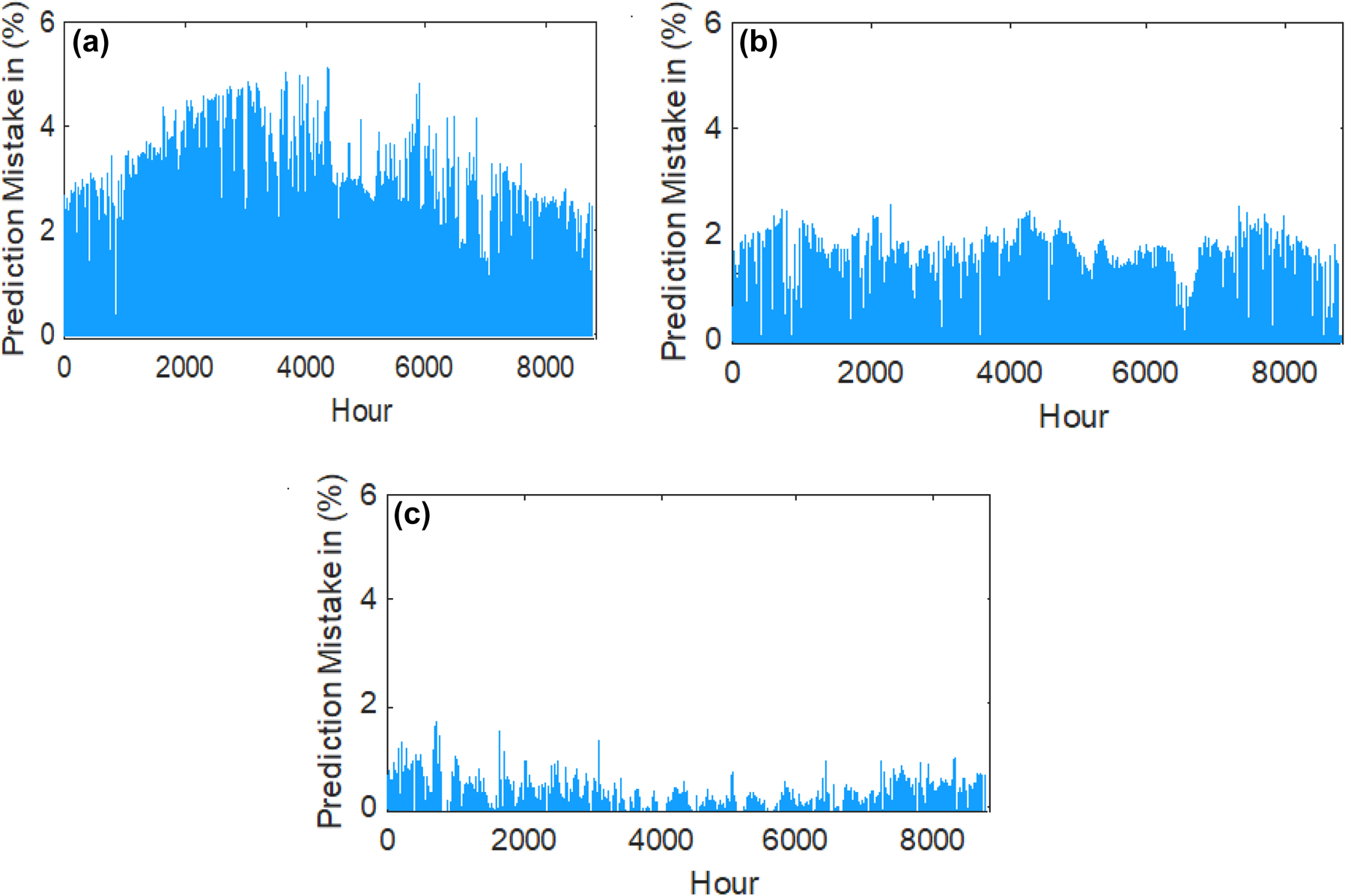
Prediction mistakes for (a) Case I, (b) Case II, (c) Ccase III.
To achieve a real assessment for the whole simulation period, the average of the prediction mistakes would be also computed. Eq. (3) shows the mathematical expression by which this average is found. Figure 8 gives the averages for the three cases in this study. Compared to (2.13% and 1.75%) found for cases I and II, it is notable that case III shows the lowest average (0.83%).

Averages of prediction mistakes for the three cases of multi-term zenith angle function.
6 Plan of energy management supported with prediction
The impact of utilizing the aforementioned predictive neural network with a multi-term zenith angle function on managing the energy consumption in solar-fed sensor units is discussed in this section. More specifically, the three cases that were listed in Table 3. However, the discussion requires a prior declaration of the working modes of the sensor units. These modes are provided in the first Subsection 6.1 for the most utilized neutrality management plan. Subsequently, an explanation for the implementation scenario, in which the predicted harvested energy is benefited, would be provided in Subsection 6.2. The last subsection presents and analyzes the allocation of the working modes during a selected simulation period.
6.1 Working modes of the sensor unit
The effects on the collected solar energy are considered slight compared to the consumed energy. For this reason, there is a big desire to regulate energy consumed in small-scale energy systems more than the collected energy. Hence, the plan for managing energy must have the ability to handle the energy delivered to the system in a well way ensuring fulfilling a permanent balance. Here, the neutrality management plan which is explained in (Al-Omary 2019; Al-Omary et al. 2022a), would be a good option to execute. This plan allows adjusting the sensor unit into one of the four working modes that appear in Figure 9.

Working modes of the neutrality management plan of energy in the sensor unit.
The movement from one mode to another depends on the level of powering energy. The working mode (M3) is the highest energy consumption. The powering energy in this mode exceeds the top limit
Because of the great consumption of energy in the persistent mode, any movement in the working modes from (M3) to (M2) will degrade the energy consumption. Conversely, the elimination of the working modes (M0 & M1) leads to more consumption of energy. In this regard, the working mode M2 is considered the most satisfactory and preferred one for being the middle mode in which fulfilling the energy balance is possible.
6.2 Implementation scenario of the sensor unit
The neutrality management plan explained in Subsection 6.1 has been included in an executed sensor unit. The implementation scenario encloses values of the energy limits that have been calculated from corresponding current values as well as the 3.3 V operating voltage for the wireless sensor unit. Table 7 offers those values for the current and the accompanied energy limits.
Values of currents and the accompanied energy limits for the implemented scenario.
| Limit of movement from working mode to another | Current value | Accompanied energy limit |
|---|---|---|
| Top limit |
|
|
| Nominal limit |
|
|
| Minimum limit |
|
|
It is worth noting that the area of the photovoltaic cell utilized in this executed sensor unit was chosen to be 5 cm2. Besides this cell, a battery is added as a storage element in this unit. Thus, the sensor unit would be fed through these two powering sources. The energy stored in the battery (E s ) is computed by the difference between the provided energy (E pro), consumed energy (E con) as well as the initial energy present in the battery (E s_ini) as in Eq. (4).
By considering individual and sequential windows of time, Eq. (4) could be rewritten as in Eq. (5).
To keep the battery safe against any extra energy harvested from the photovoltaic cell, the maximum capacity of the battery (E s_max) is considered here. This safety procedure is mathematically translated, as shown in Eq. (6).
6.3 Incidence times of working modes
This subsection shows the number of times at which the working modes are incident when a sensor unit with the management plan in Subsection 6.1 and the implementation scenario in Subsection 6.2 is used for one month (from 15th Jan 2022 to 14th Feb 2022) in Amman city. To identify the impact of using a multi-term zenith angle function, the incidence time would be recorded for the three cases mentioned in Subsection 5.2. Since the prediction in hourly resolution is assumed for all the cases, there would be 720 working hours for this month. Figure 10 shows how these hours would be allocated among the working modes explained in Subsection 6.1. Additionally, it indicates that the sensor unit has never been turned off during the mentioned month as the mode (M0) did not occur at all for any case. This means that the node worked effectively because of the permanent operation. On the other hand, the node was at rest (works at mode M1) for 24 h during this month in all cases. Thus, the node will consume the same amount of energy in the three cases. (i.e., no case will consume more or less energy than others).

Allocating the incidence times on the working modes of a sensor unit using predictive neural network with three cases of multi-term zenith angle function during the period (15th Jan 2022 to 14th Feb 2022).
The cases appear a disparity in the incidence time of the working mode (M2). Here, (688, 691, and 695) hours have been recorded respectively for cases I, II and III. It is worth pointing out that while there is a remarkable decrease in the incidence times from case III toward case I, this decrease is accompanied by an increase in the incidence times of the working mode (M3). It can be observed from Figure 10 that the incidence times of the working mode (M3) are (1, 5, and 8) hours for cases III, II, and I, respectively. Taken together, all these numbers indicate that case III, in which the neural network uses a zenith angle function of four terms, has less total energy consumption than case II which only uses three terms. Additionally, case II has less energy consumption than case I (the case of two terms) in total. Consequently, case III would be the most suitable case for fulfilling more effective work (less consumption and full action) for the sensor node.
7 Conclusion
Solar-harvesting sensor nodes could not be a sustainable technology to a sufficient degree without operating these nodes effectively. Because of the intermittent nature of solar energy, reaching the point of effective operation is considered a challenge. The low energy consumption with full and constant functions for the nodes supports reaching this point. The neural networks-based prediction contributes to achieving well-management of the energy consumed by these nodes. One of the neural networks used with solar-harvesting sensor nodes adopts the zenith angle function as input. This paper has investigated the impact of using the zenith angle function with multi-term on energy management in this technology. To this end, three cases (two, three and four terms) have been addressed and employed in an executed node. The results have proven that increasing the terms for the zenith angle function would remarkably improve the manageability level. In other words, it will push solar-harvesting sensor nodes toward less consumption and effective working.
Nomenclature
- cm2
-
Squared centimeter
- E(i, j)
-
Matrix of energy profiles
- EWMA
-
Exponentially weighted moving average
- E con
-
Energy consumed by the wireless sensor
- E pro
-
Energy supplied to the wireless sensor
- E min
-
Initial energy level where the wireless sensor starts working in the sleep mode
- E n
-
Nominal energy level
- E s
-
Energy stored in the battery
- E s_ini
-
Energy available in the battery at the initial state
- E s_max
-
Maximum energy level of the battery
- GAP
-
Scaling factor reflects the current day solar condition relative to the past days
- GSR
-
Global solar radiation
- I min
-
Current level at the wireless sensor starts working in the sleep mode
- I n
-
Nominal current level.
- J
-
Joule
- J/h
-
Joule per hour
- μ
-
Micro (10–6)
- m
-
Milli (10–3)
- M D (d, n)
-
Mean value of energy harvested at time window
- M0
-
Switch off operating mode
- M1
-
Sleep operating mode
- M2
-
Active operating mode
- M3
-
Continuous operating mode
- n
-
Time window in a day
- n + 1
-
Predictable time window
- R
-
Correlation coefficient
- R 2
-
Coefficient of determination
- s
-
Second
- T
-
Total number of hourly GSR samples
- W
-
Watt
- WCMA
-
Weather conditioned moving average
- x t
-
Measured GSR at specific hour t
- y t
-
Predicted GSR at specific hour t
- θ z
-
Zenith angle.
- α
-
Weighting factor.
Funding source: German Jordanian University, Deanship of Scientific Research
Award Identifier / Grant number: SNREM19/2021
-
Author contributions: Murad Al-Omary: Project administration, Conceptualization, Methodology, Resources, Supervision, Formal analysis, Investigation, Writing – Original Draft. Rafat Aljarrah: Data Curation, Software, Validation, Writing – Review & Editing. Aiman Albatayneh: Visualization, Writing – Review & Editing. Dua’a Alshabi: Writing – Original Draft. Khaled Alzaareer: Writing – Review & Editing.
-
Research funding: The authors thank German Jordanian University for providing financial support through the Seed Grant (SNREM 19/2021) to buy the equipment that contributed to achieving this work.
-
Conflicts of interest statement: The authors declared that there are no conflicts of interest.
References
Azeem, N. S. A., I. Tarrad, A. A. Hady, M. I. Youssef, and S. M. A. El-kader. 2019. “Shared Sensor Networks Fundamentals, Challenges, Opportunities, Virtualization Techniques, Comparative Analysis, Novel Architecture and Taxonomy.” JSAN 8 (2): 29. https://doi.org/10.3390/jsan8020029.Search in Google Scholar
Avtar, N. Sahu, Aggarwal, S. Chakraborty, A. Kharrazi, A. P. Yunus, J. Dou, and Kurniawan. 2019. “Exploring Renewable Energy Resources Using Remote Sensing and GIS—A Review.” Resources 8 (3): 149. https://doi.org/10.3390/resources8030149.Search in Google Scholar
Al_Omary, M. S. M. 2019. Accuracy Improvement of Predictive Neural Networks for Managing Energy in Solar Powered Wireless Sensor Nodes. Chemnitz, Germany: Technical University of Chemnitz.Search in Google Scholar
Al-Omary, M., K. Hassini, A. Fakhfakh, and O. Kanoun 2019. “Prediction of Energy in Solar Powered Wireless Sensors Using Artificial Neural Network.” In 2019 16th International Multi-Conference on Systems, Signals & Devices (SSD), 288–93. IEEE.confproc10.1109/SSD.2019.8893213Search in Google Scholar
Al-Omary, M., R. Aljarrah, A. Albatayneh, and H. Jaradat 2021. “A Composite Moving Average Algorithm for Predicting Energy in Solar Powered Wireless Sensor Nodes.” In 2021 18th International Multi-Conference on Systems, Signals & Devices (SSD), 1047–52. IEEE.confproc10.1109/SSD52085.2021.9429440Search in Google Scholar
Al-Omary, M., A. Albatayneh, H. Jaradat, and R. Aljarrah 2022a. “An Efficient Energy-Aware Controller for Small-Scale Solar-Worked Devices Using Ratioed Pro-energy Predictor.” In 2022 IEEE Electrical Power and Energy Conference (EPEC), 336–41. IEEE.confproc10.1109/EPEC56903.2022.10000232Search in Google Scholar
Al-Omary, M., R. Aljarrah, A. Albatayneh, K. Alzaareer, A. Malkawi, and H. Jaradat. 2022b. “Optimal Neural Network for Predicting Solar Energy in Sensor Units Based on a Cascaded Input/Structure Direct Optimization.” Journal of Sensors 2022: 1–18. https://doi.org/10.1155/2022/7273469.Search in Google Scholar
Al-Omary, M., A. Albatayneh, R. Aljarrah, and K. Alzaareer. 2022c“Reliability Evaluation of GSR Prediction Using Neural Networks with Variant Atmospheric Parameters.” In 2022 19th International Multi-Conference on Systems, Signals & Devices (SSD), 1156–61. IEEE.confproc10.1109/SSD54932.2022.9955790Search in Google Scholar
Al-Omary, M., M. Kaltschmitt, and C. Becker. 2018. “Electricity System in Jordan: Status & Prospects.” Renewable and Sustainable Energy Reviews 81: 2398–409. https://doi.org/10.1016/j.rser.2017.06.046.Search in Google Scholar
Bergonzini, C., D. Brunelli, and L. Benini. 2010. “Comparison of Energy Intake Prediction Algorithms for Systems Powered by Photovoltaic Harvesters.” Microelectronics Journal 41 (11): 766–77. https://doi.org/10.1016/j.mejo.2010.05.003.Search in Google Scholar
Bouguera, T., J.-F. Diouris, G. Andrieux, J.-J. Chaillout, and R. Jaouadi. 2018. “A Novel Solar Energy Predictor for Communicating Sensors.” IET Communications 12 (17): 2145–9. https://doi.org/10.1049/iet-com.2018.5244.Search in Google Scholar
Carlos-Mancilla, M., E. López-Mellado, and M. Siller. 2016. “Wireless Sensor Networks Formation: Approaches and Techniques.” Journal of Sensors 2016: 1–18. https://doi.org/10.1155/2016/2081902.Search in Google Scholar
Cammarano, A., C. Petrioli, and D. Spenza. 2012. “Pro-Energy: A Novel Energy Prediction Model for Solar and Wind Energy-Harvesting Wireless Sensor Networks.” In 2012 IEEE 9th International Conference on Mobile Ad-Hoc and Sensor Systems (MASS 2012), 75–83. IEEE.confproc10.1109/MASS.2012.6502504Search in Google Scholar
Cammarano, A., C. Petrioli, and D. Spenza. 2016. “Online Energy Harvesting Prediction in Environmentally Powered Wireless Sensor Networks.” IEEE Sensors Journal 16 (17): 6793–804. https://doi.org/10.1109/JSEN.2016.2587220.Search in Google Scholar
Dehwah, A. H., S. Elmetennani, and C. Claudel. 2017. “UD-WCMA: An Energy Estimation and Forecast Scheme for Solar Powered Wireless Sensor Networks.” Journal of Network and Computer Applications 90: 17–25. https://doi.org/10.1016/j.jnca.2017.04.003.Search in Google Scholar
Deb, M., and S. Roy. 2021. “Enhanced-Pro: A New Enhanced Solar Energy Harvested Prediction Model for Wireless Sensor Networks.” Wireless Personal Communications 117 (2): 1103–21. https://doi.org/10.1007/s11277-020-07913-y.Search in Google Scholar
Engmann, F., K. Sarpong Adu-Manu, J.-D. Abdulai, and F. Apietu Katsriku. 2021. “Applications of Prediction Approaches in Wireless Sensor Networks.” In Wireless Sensor Networks – Design, Deployment and Applications, edited by S. S. Yellampalli. IntechOpen.book-chapter10.5772/intechopen.94500Search in Google Scholar
Edalat, N., and M. Motani. 2016. “Energy-aware Task Allocation for Energy Harvesting Sensor Networks.” Journal of Wireless Communications and Networking 2016 (1): 1–14, https://doi.org/10.1186/s13638-015-0490-3.Search in Google Scholar
Galar, D., and U. Kumar. 2017. “Sensors and Data Acquisition.” In eMaintenance, 1–72. Elsevier.book-chapter10.1016/B978-0-12-811153-6.00001-4Search in Google Scholar
Goyal, D. and Sonal, eds. 2016. Power Management in Wireless Sensor Network. IEEE.book-chapterSearch in Google Scholar
Ghuman, M. F., A. Iqbal, H. K. Qureshi, and M. Lestas. 2015. “ASIM.” In Proceedings of the 3rd International Workshop on Energy Harvesting & Energy Neutral Sensing Systems, edited by G. V. Merrett, C. Renner, and D. Brunelli, Vol. 11, 21–6. New York: ACM.10.1145/2820645.2820646Search in Google Scholar
Hassan, M. and A. Bermak. 2012. “Solar Harvested Energy Prediction Algorithm for Wireless Sensors.” In 2012 Asia Symposium on Quality Electronic Design (ASQED), 178–81. IEEE.confproc10.1109/ACQED.2012.6320497Search in Google Scholar
Jankovic, S., and L. Saranovac. 2020. “Prediction of Harvested Energy for Wireless Sensor Node.” Elektronica and Elektrotechniek 26 (1): 23–31. https://doi.org/10.5755/j01.eie.26.1.23807.Search in Google Scholar
Jiang, Z., X. Jin, and Y. Zhang. 2010. “A Weather-Condition Prediction Algorithm for Solar-Powered Wireless Sensor Nodes.” In 2010 International Conference on Computational Intelligence and Software Engineering. Vol. 23, 1–4. IEEE.confproc10.1109/WICOM.2010.5601116Search in Google Scholar
Kansal, A., J. Hsu, S. Zahedi, and M. B. Srivastava. 2007. “Power Management in Energy Harvesting Sensor Networks.” ACM Transactions on Embedded Computing Systems 6 (4): 32. https://doi.org/10.1145/1274858.1274870.Search in Google Scholar
Khan, J. A., H. K. Qureshi, and A. Iqbal. 2015. “Energy Management in Wireless Sensor Networks: A Survey.” Computers & Electrical Engineering 41: 159–76. https://doi.org/10.1016/j.compeleceng.2014.06.009.Search in Google Scholar
Kosunalp, S. 2016. “A New Energy Prediction Algorithm for Energy-Harvesting Wireless Sensor Networks with Q-Learning.” IEEE Access 4: 5755–63. https://doi.org/10.1109/ACCESS.2016.2606541.Search in Google Scholar
Liang, Y., C. -Z. Zhao, H. Yuan, Y. Chen, W. Zhang, J. -Q. Huang, D. Yu, Y. Liu, M. Titirici, Y. Chueh, H. Yu, and Q. Zhang. 2019. “A Review of Rechargeable Batteries for Portable Electronic Devices.” InfoMat 1 (1): 6–32. https://doi.org/10.1002/inf2.12000.Search in Google Scholar
Li, Y., and R. Shi. 2015. “An Intelligent Solar Energy-Harvesting System for Wireless Sensor Networks.” Journal of Wireless Communications and Networking 2015 (1): 1–12, https://doi.org/10.1186/s13638-015-0414-2.Search in Google Scholar
Lorincz, J., A. Capone, and J. Wu. 2019. “Greener, Energy-Efficient and Sustainable Networks: State-Of-The-Art and New Trends.” Sensors 19 (22): 1–29, https://doi.org/10.3390/s19224864.Search in Google Scholar PubMed PubMed Central
Le, T. N., O. Sentieys, O. Berder, A. Pegatoquet, and C. Belleudy, eds. 2013. Adaptive Filter For Energy Predictor in Energy Harvesting Wireless Sensor Networks.IEEE.book-chapter10.1109/GreenCom.2012.107Search in Google Scholar
Matin, M. A., and M. M. Islam. 2012. “Overview of Wireless Sensor Network.” In Wireless Sensor Networks – Technology and Protocols, edited by M. Matin. InTech.book-chapter.10.5772/49376Search in Google Scholar
Munir, B., and V. Dyo. 2018. “On the Impact of Mobility on Battery-Less RF Energy Harvesting System Performance.” Sensors 18 (11): 1–16, https://doi.org/10.3390/s18113597.Search in Google Scholar PubMed PubMed Central
Mabon, M., M. Gautier, B. Vrigneau, M. Le Gentil, and O. Berder. 2019. “The Smaller the Better: Designing Solar Energy Harvesting Sensor Nodes for Long-Range Monitoring.” Wireless Communications and Mobile Computing 2019: 1–11. https://doi.org/10.1155/2019/2878545.Search in Google Scholar
Piorno, J. R., C. Bergonzini, D. Atienza, and T. R. Simunic. 2009. “Prediction and Management in Energy Harvested Wireless Sensor Nodes.” In 2009 1st International Conference on Wireless Communication, Vehicular Technology, Information Theory and Aerospace & Electronic Systems Technology, 6–10. IEEE.confproc10.1109/WIRELESSVITAE.2009.5172412Search in Google Scholar
Prauzek, M., J. Konecny, M. Borova, K. Janosova, J. Hlavica, and P. Musilek. 2018. “Energy Harvesting Sources, Storage Devices and System Topologies for Environmental Wireless Sensor Networks: A Review.” Sensors 18 (8): 1–22, https://doi.org/10.3390/s18082446.Search in Google Scholar PubMed PubMed Central
Ren, H., J. Guo, L. Sun, and C. Han. 2018. “Prediction Algorithm Based on Weather Forecast for Energy-Harvesting Wireless Sensor Networks.” In 2018 17th IEEE International Conference on Trust, Security and Privacy in Computing and Communications/12th IEEE International Conference on Big Data Science and Engineering (TrustCom/BigDataSE), 1785–90. IEEE.confproc10.1109/TrustCom/BigDataSE.2018.00269Search in Google Scholar
Senouci, M. R., and A. Mellouk. 2016. “Wireless Sensor Networks.” In Deploying Wireless Sensor Networks, 1–19. Elsevier.book-chapter10.1016/B978-1-78548-099-7.50001-5Search in Google Scholar
Sah, D. K., and T. Amgoth. 2020. “Renewable Energy Harvesting Schemes in Wireless Sensor Networks: A Survey.” Information Fusion 63: 223–47. https://doi.org/10.1016/j.inffus.2020.07.005.Search in Google Scholar
Sharma, H., A. Haque, and Z. A. Jaffery. 2018. “Solar Energy Harvesting Wireless Sensor Network Nodes: A Survey.” Journal of Renewable and Sustainable Energy 10 (2): 23704. https://doi.org/10.1063/1.5006619.Search in Google Scholar
Silva, A., M. Liu, and M. Moghaddam. 2012. “Power-Management Techniques for Wireless Sensor Networks and Similar Low-Power Communication Devices Based on Nonrechargeable Batteries.” Journal of Computer Networks and Communications 2012: 1–10. https://doi.org/10.1155/2012/757291.Search in Google Scholar
Srinivas, Y., A. S. Raj, D. H. Oliver, D. Muthuraj, and N. Chandrasekar. 2012. “A Robust Behavior of Feed Forward Back Propagation Algorithm of Artificial Neural Networks in the Application of Vertical Electrical Sounding Data Inversion.” Geoscience Frontiers 3 (5): 729–36. https://doi.org/10.1016/j.gsf.2012.02.003.Search in Google Scholar
Thakur, S., D. Prasad, and A. Verma. 2017. “Energy Harvesting Methods in Wireless Sensor Network: A Review.” IJCA 165 (9): 19–22. https://doi.org/10.5120/ijca2017914000.Search in Google Scholar
Xia, F. 2009. “Wireless Sensor Technologies and Applications.” Sensors 9 (11): 8824–30. https://doi.org/10.3390/s91108824.Search in Google Scholar PubMed PubMed Central
Xu, X., J. Tang, and H. Xiang. 2022. “Data Transmission Reliability Analysis of Wireless Sensor Networks for Social Network Optimization.” Journal of Sensors 2022: 1–12. https://doi.org/10.1155/2022/3842722.Search in Google Scholar
Zou, T., W. Xu, W. Liang, J. Peng, Y. Cai, and T. Wang. 2017. “Improving Charging Capacity for Wireless Sensor Networks by Deploying One Mobile Vehicle with Multiple Removable Chargers.” Ad Hoc Networks 63: 79–90. https://doi.org/10.1016/j.adhoc.2017.05.006.Search in Google Scholar
Zou, T., S. Lin, Q. Feng, and Y. Chen. 2016. “Energy-Efficient Control with Harvesting Predictions for Solar-Powered Wireless Sensor Networks.” Sensors 16 (1): 1–31, https://doi.org/10.3390/s16010053.Search in Google Scholar PubMed PubMed Central
© 2024 the author(s), published by De Gruyter, Berlin/Boston
This work is licensed under the Creative Commons Attribution 4.0 International License.
Articles in the same Issue
- Solar photovoltaic-integrated energy storage system with a power electronic interface for operating a brushless DC drive-coupled agricultural load
- Analysis of 1-year energy data of a 5 kW and a 122 kW rooftop photovoltaic installation in Dhaka
- Reviews
- Real yields and PVSYST simulations: comparative analysis based on four photovoltaic installations at Ibn Tofail University
- A comprehensive approach of evolving electric vehicles (EVs) to attribute “green self-generation” – a review
- Exploring the piezoelectric porous polymers for energy harvesting: a review
- A strategic review: the role of commercially available tools for planning, modelling, optimization, and performance measurement of photovoltaic systems
- Comparative assessment of high gain boost converters for renewable energy sources and electrical vehicle applications
- A review of green hydrogen production based on solar energy; techniques and methods
- A review of green hydrogen production by renewable resources
- A review of hydrogen production from bio-energy, technologies and assessments
- A systematic review of recent developments in IoT-based demand side management for PV power generation
- Research Articles
- Hybrid optimization strategy for water cooling system: enhancement of photovoltaic panels performance
- Solar energy harvesting-based built-in backpack charger
- A power source for E-devices based on green energy
- Theoretical and experimental investigation of electricity generation through footstep tiles
- Experimental investigations on heat transfer enhancement in a double pipe heat exchanger using hybrid nanofluids
- Comparative energy and exergy analysis of a CPV/T system based on linear Fresnel reflectors
- Investigating the effect of green composite back sheet materials on solar panel output voltage harvesting for better sustainable energy performance
- Electrical and thermal modeling of battery cell grouping for analyzing battery pack efficiency and temperature
- Intelligent techno-economical optimization with demand side management in microgrid using improved sandpiper optimization algorithm
- Investigation of KAPTON–PDMS triboelectric nanogenerator considering the edge-effect capacitor
- Design of a novel hybrid soft computing model for passive components selection in multiple load Zeta converter topologies of solar PV energy system
- A novel mechatronic absorber of vibration energy in the chimney
- An IoT-based intelligent smart energy monitoring system for solar PV power generation
- Large-scale green hydrogen production using alkaline water electrolysis based on seasonal solar radiation
- Evaluation of performances in DI Diesel engine with different split injection timings
- Optimized power flow management based on Harris Hawks optimization for an islanded DC microgrid
- Experimental investigation of heat transfer characteristics for a shell and tube heat exchanger
- Fuzzy induced controller for optimal power quality improvement with PVA connected UPQC
- Impact of using a predictive neural network of multi-term zenith angle function on energy management of solar-harvesting sensor nodes
- An analytical study of wireless power transmission system with metamaterials
- Hydrogen energy horizon: balancing opportunities and challenges
- Development of renewable energy-based power system for the irrigation support: case studies
- Maximum power point tracking techniques using improved incremental conductance and particle swarm optimizer for solar power generation systems
- Experimental and numerical study on energy harvesting performance thermoelectric generator applied to a screw compressor
- Study on the effectiveness of a solar cell with a holographic concentrator
- Non-transient optimum design of nonlinear electromagnetic vibration-based energy harvester using homotopy perturbation method
- Industrial gas turbine performance prediction and improvement – a case study
- An electric-field high energy harvester from medium or high voltage power line with parallel line
- FPGA based telecommand system for balloon-borne scientific payloads
- Improved design of advanced controller for a step up converter used in photovoltaic system
- Techno-economic assessment of battery storage with photovoltaics for maximum self-consumption
- Analysis of 1-year energy data of a 5 kW and a 122 kW rooftop photovoltaic installation in Dhaka
- Shading impact on the electricity generated by a photovoltaic installation using “Solar Shadow-Mask”
- Investigations on the performance of bottle blade overshot water wheel in very low head resources for pico hydropower
- Solar photovoltaic-integrated energy storage system with a power electronic interface for operating a brushless DC drive-coupled agricultural load
- Numerical investigation of smart material-based structures for vibration energy-harvesting applications
- A system-level study of indoor light energy harvesting integrating commercially available power management circuitry
- Enhancing the wireless power transfer system performance and output voltage of electric scooters
- Harvesting energy from a soldier's gait using the piezoelectric effect
- Study of technical means for heat generation, its application, flow control, and conversion of other types of energy into thermal energy
- Theoretical analysis of piezoceramic ultrasonic energy harvester applicable in biomedical implanted devices
- Corrigendum
- Corrigendum to: A numerical investigation of optimum angles for solar energy receivers in the eastern part of Algeria
- Special Issue: Recent Trends in Renewable Energy Conversion and Storage Materials for Hybrid Transportation Systems
- Typical fault prediction method for wind turbines based on an improved stacked autoencoder network
- Power data integrity verification method based on chameleon authentication tree algorithm and missing tendency value
- Fault diagnosis of automobile drive based on a novel deep neural network
- Research on the development and intelligent application of power environmental protection platform based on big data
- Diffusion induced thermal effect and stress in layered Li(Ni0.6Mn0.2Co0.2)O2 cathode materials for button lithium-ion battery electrode plates
- Improving power plant technology to increase energy efficiency of autonomous consumers using geothermal sources
- Energy-saving analysis of desalination equipment based on a machine-learning sequence modeling