Non-transient optimum design of nonlinear electromagnetic vibration-based energy harvester using homotopy perturbation method
-
Aboozar Dezhara


Abstract
In this paper the coupled differential equations governing the vibration of nonlinear electromagnetic energy harvesters are solved by the homotopy perturbation method. The amplitudes of odd harmonics of displacement of the magnet, coil current, and load voltage are derived up to the 5th harmonic. The frequency response of output power is plotted and it peaks at the linear mechanical resonance frequency. It should be noted that the optimum design of coil and load parameters, optimum electromagnetic coupling coefficient, and optimum vibration frequency of the magnet attached to a non-linear spring resulted in a stationary or non-transient vibration. Paying insufficient attention to this point and using typical parameters instead of optimum ones will result in transient vibration. The research aims at a rigorous semi-analytical method on a nonlinear problem which has previously solely investigated by numerical or experimental method.
1 Introduction
The enormous growth has been witnessed in the realm of wireless devices in the past few decades. But, in many cases, the extent of services rendered by these devices has been dictated by the lifetime of batteries powering them. Presence of a self-sustainable power source would thus enable the exploitation of the full potential of such devices. Miniaturization is the prime motive behind the current technological revolution and as devices continue to shrink, less energy is required onboard (kamaraj, Ali, and Arockiarajan 2015). Nonlinear vibration frequently occurs in engineering problems among them the problem of nonlinear electromagnetic energy harvesters with spring non-linearity received substantial attention recently because of their high output power at the low resonance frequency. In this paper, the new perturbation method called the homotopy perturbation method is proposed, in contrast to the traditional perturbation methods, this technique does not require a small parameter in an equation. In this method, according to the homotopy technique, a homotopy with an embedding parameter p is constructed, and the embedding parameter is considered as 1, so the method is called the homotopy perturbation method, which can take full advantage of the traditional perturbation methods and homotopy techniques. To illustrate its effectiveness and its convenience, a Duffing equation with high order of nonlinearity is used (Anjum and He 2020; He 2000, 2003; Yu, He, and García 2019). Many researchers work on this subject without paying much attention to the optimum design of these harvesters so they design a harvester that vibrates with specified mechanical parameters at specified base acceleration and gives specified electrical power at generally their mechanical resonance frequency, and with the same mechanical as well as electrical parameters, these devices give different output power!. However, in this paper and the author’s previous paper (Dezhara 2022a) it is proved that with the same parameters different output power can not be achieved with different mechanical configurations. With optimum parameters, the frequency response will peak at the mechanical resonance frequency for nonlinear vibration-based harvesters, but no power will be delivered to electrical loads for linear ones because efficiency is zero at the mechanical resonance frequency. Generally, it is difficult to provide an exact or closed-form solution to nonlinear dynamical equations. Therefore, researchers have attempted to implement approximate analytical solutions or numerical solutions for such equations. Approximate solutions provide important information to understand the characteristics of mechanical systems, specifically during the design procedure (Bayat et al. 2022). Li and Lim (Ghadimi and Kaliji 2013) applied Newton–harmonic balance (NHB) to the nonlinear oscillation systems to yield an approximate analytical expression for large amplitude problems. The accuracy of the high order of the NHB was verified, and it is not restricted to small and large positive parameters of the Duffing equation. Bayat, Pakar, and Cveticanin (2014) proposed the Hamiltonian Approach to achieve an accurate solution for nonlinear ordinary differential equations with inertia and static-type cubic nonlinearities. Their proposed solution is accurate for the whole domain. Homotopy perturbation Method (HPM) was first proposed by He (1999) and is widely used in nonlinear problems. Ganji, Tari, and Jooybari (2007) extended the HMP for nonlinear evolution equations and compared the results with the variational iteration method. Among all mentioned approaches, the Homotopy Perturbation Method (HPM) has been used widely for nonlinear systems. Compared to other approaches, it has the following advantages: (a) It is appropriate to be used for strong nonlinear oscillators, and (b) the solving procedure in higher order approximation is quite simple. In this paper, the high-order approximate Homotopy Perturbation Method (HPM) is developed to evaluate the nonlinear frequency response of an electromagnetic vibration-based energy harvester (EVEH) at a capacitive load. The governing equation of motion consists of three coupled differential equations one of them are second-order nonlinear differential equation and the other two equations are linear first-order differential equations. The coupled equations with linear and nonlinear properties are transformed into a set of differential–algebraic equations using intermediate variables. The obtained differential–algebraic equations are solved by HPM. It has been demonstrated the second order of the HPM can lead us to a highly accurate solution that is valid for the whole domain of the problem. It should be noted that in the view of mathematics, this research is novel research of its kind because the other researchers paid no or little attention to solving coupled differential equations using HPM (Figures 1 and 2).

Typical nonlinear electromagnetic energy harvester (reprinted from reference (Kubba and Jiang 2014)).
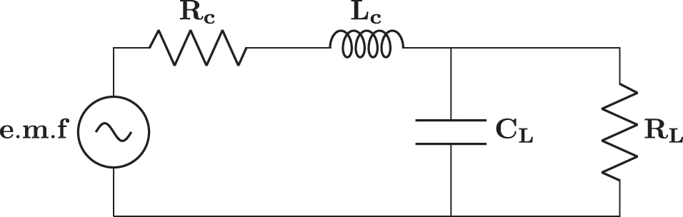
EVEH’s electrical side for capacitive load.
2 Homotopy perturbation method
The coupled differentials equations of EVEH (Figure 1) are as follows (Aldawood, Nguyen, and Bardaweel 2019) (see Figure 2):
where the z is magnet displacement and the i is coil current and the v is load voltage, C m , K, m, A b , k 1, k 3 are mechanical damping coefficient, electromagnetic coupling coefficient, the mass of the magnet, base acceleration, linear spring constant, and nonlinear spring constant respectively. It should be noted that in our analysis the sign of coefficients of k 1 and k 3 are not necessarily positive and they may possess negative values. In solving these coupled equations you should note that in arranging the homotopy equation of nonlinear differential equation of (1) the zero-order homotopy variable equation should be simple harmonic so that you will be able to solve higher-order homotopy variable differential equations. Consequently, the author arranges the first equation i.e. equation of (1) as follows:
where the prime and dot are derivative with respect to time. Now write the initial conditions according to homotopy theory:
Similarly the derivative of v and i at time t = 0 is zero. Note that we just expand the number of zero to homotopy variable p for z and not for i or v (the reason will be known later in this paper). Consequently, we have these initial conditions and relations:
By substituting equations of (5), (6), (7) into Equation (4):
It should be noted that the first equation in (16) is a simple harmonic equation, second and third equations in (16) are coupled with current. To solve these coupled equations you should refer to other differential equations i.e. equations of (2) and (3). Accordingly, we proceed as follows: The solution of the first differential equation of (16) is:
For solving the second differential equation you should first solve for i 0 and with known z 0 and i 0 one can solve for z 1. Now write the homotopy equation for equations of (2) and (3). For convenience, we can assume the prime is a symbol of the derivative with respect to time for coil current and load voltage. According to the equation of (3):
According to the Equation (2):
Now consider the first equation of (19) and combine it with the first equation of (21) and eliminate i 0. As we know z 0 from the equation of (17), we can solve for v 0 and consequently i 0. we proceed as follows. First eliminate i 0:
If you solve for v 0 and substitute it in the first equation of (19) the i 0 will be obtained and consequently we can solve for z 1 from the second equation of (16). The reason for not expanding the zero initial condition of v and i now became known, the differential equation of v has a damping term and the transient response of it became evanescent as time goes by, hence we assumed all initial conditions of v and i are zero. However, the z has not this condition i.e. has not had the damping term. Now turn to the differential equation of (22):
The forced response of the above equation is as follows:
By substituting the above equation into the differential equation of (24) we have:
where α 1, α 2, and α 3 are coefficients of derivatives in the equation of (24).
By arranging equation of (26) we have:
In the matrix form, we have:
Now that the v 0 is known we derive i 0 using the first equation of (19).
where λ 1 and λ 2 are arbitrary names for coefficients of i 0. Turning to second Equation (16) i.e. differential equation of z 1, we have:
putting the i 0 into the above differential equation:
To avoid secular terms the coefficients of cos(ωt) and sin(ωt) at the right side of Equation (35) should be equaled to zero.
From the equation of (36) the value of unknown parameter a 1 will be known. And from the equation of (37), the value of Z 0 will be known.
After omitting the secular terms the differential equation of z 1 is:
Now we can solve for the z 1, assume the forced response of z 1 is:
putting the equation of (41) into the Equation (40), we have:
The result is:
The general solution of z 1 is:
Hence we have:
Now turn to the third differential equation of (16), we should first derive i 1 and then solve for z 2. Combining i 1 into the second equation of (19) and as we derived z 1 we can solve for v 1 and consequently i 1.
assume v 1 as:
By substituting (48) into the differential equation of (47), we have:
After solving the above matrix equation symbolically in MATLAB we have:
From the second equation of (19) we have:
where:
Turning to third Equation (16) i.e. differential equation for z 2, we have:
By substituting the i 1 into the above differential equation:
The multiplication action between the two big parentheses on the right-hand side of the differential equation of (53) can be simplified as follows:
Finally, after simplifying the above term the differential equation became:
To avoid secular terms the coefficients of cos(ωt) and sin(ωt) at the right side of Equation (54) should be equaled to zero.
These equations are vital in the design process. We will use them directly without simplification in MALTAB to derive optimum parameters numerically.
Thus Equation (54) became:
where:
Now we can solve for the z 2, assume z 2 is:
By substituting Equation (62) into Equation (57) and after simplifying we can solve for constants of D 2, E 2, F 2 and G 2.
Applying initial conditions we have:
Hence:
To derive v 2 from the third equation of (19) eliminate i 2 from this equation using the third equation of (18).
since z 2 has the cos(3ωt) and cos(5ωt) terms we can assume v 2 as follows:
By putting (70) into the Equation (69) and simplifying the resulted relations we have:
you can solve the above matrix equation in MATLAB symbolically, the result is:
where δ 3, δ 4 and δ 5 are:
Now that we know v 2 we can derive i 2 from third equation of (18):
where the constants are as follows:
Now you can add these currents or voltages or even displacements to achieve the unknowns dependent variables in coupled differential equations. If we take the homotopy variable (p) as (1), we have:
where a 1 and a 2 obtained from relations of (38) and (56) or (55) respectively. The displacement of magnet is:
The coil current is:
The load voltage is:
The resonance frequency is:
To plot frequency response after designing the optimum parameters of the system you should refer to relation (90). Note that the Equation (90) is a function of Z
1, V
0, V
1, in order to eliminate these parameters and derive frequency with respect to just Z
0 and plotting frequency response you should solve symbolically (4) equations from omitting secular terms with (6) symbolic variables i.e. ω, a
1, a
2, Z
1, V
0, V
1 and two initial homotopy relation (i.e. relations of (13) and (14)) which itself add two more parameters of Z
2 and V
2 which totally became six equation and eight parameters. The other two equation comes from the first two initial conditions i.e. z(0) = 0 and
The initial conditions are:
To design optimum parameters of the system, we have (6) equations from initial conditions, (2) equations from initial homotopy relations i.e. equations of (13) and (14) plus (4) equations as a result of omitting the secular terms and one equation of frequency-amplitude i.e. relation of (90) which add up to (13) equations with (13) unknowns. Theses unknown includes R L , C L , R c , L c , ω, a 1, a 2 and (6) unknown from initial homotopy parameters. Solving these (13) nonlinear equations with (13) unknowns using fsolve command in MATLAB results in optimum parameters. Consequently, the amplitudes of sinusoidal terms of v, i, and z can be calculated.
It should be noted that the amplitudes of v, i, z are functions of (4) coil and load parameters i.e. R L , C L , R c , L c and frequency as well as initial homotopy parameters i.e. Z 0, Z 1, Z 2 and V 0, V 1, V 2.
3 Numerical example
In this example with just known values of spring constants of k 1 and k 3 and the mass of the magnet, we will design the (9) optimum parameters that lead to non-transient vibration and give us the maximum output power at this stationary situation. Consider the values of k 1, k 3 and m as follows:
Known values (g = 9.81
| Known parameter | Value | Unit |
|---|---|---|
| k 1 | 700 |
|
| k 3 | 60 |
|
| m | 14 | gr |
| C m | 0.35 |
|
| K | 3.5 |
|
| A b | 1.8 g |
|
According to our design procedure and based on MATLAB calculation the optimum parameters that lead to stationary or non-transient vibration are (Table 2):
Optimum parameters for known values of Table 1.
| Number | Optimum parameter | Value | Unit |
|---|---|---|---|
| 1 | R L | 28.5 | kΩ |
| 2 | C L | 5.14 | nF |
| 3 | R c | 10.38 | Ω |
| 4 | L c | 1.8075 | H |
| 5 | w | 223.6 |
|
| 6 | a 1 | −7.64 |
|
| 7 | a 2 | 10.45 |
|
| 8 | Z 0 | −3.2 | mm |
| 9 | Z 1 | 4 | mm |
| 10 | Z 2 | −0.883 | mm |
| 11 | V 0 | −793.1 |
|
| 12 | V 1 | 790.3 |
|
| 13 | V 2 | 2.8 |
|
The frequency response based on the above parameters is as follows (Figures 3 –7):

First harmonic displacement frequency response.
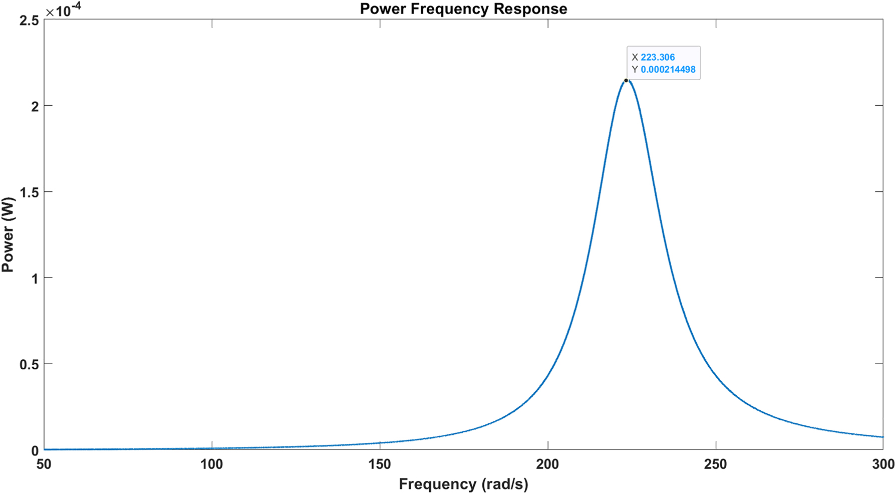
Power frequency response.
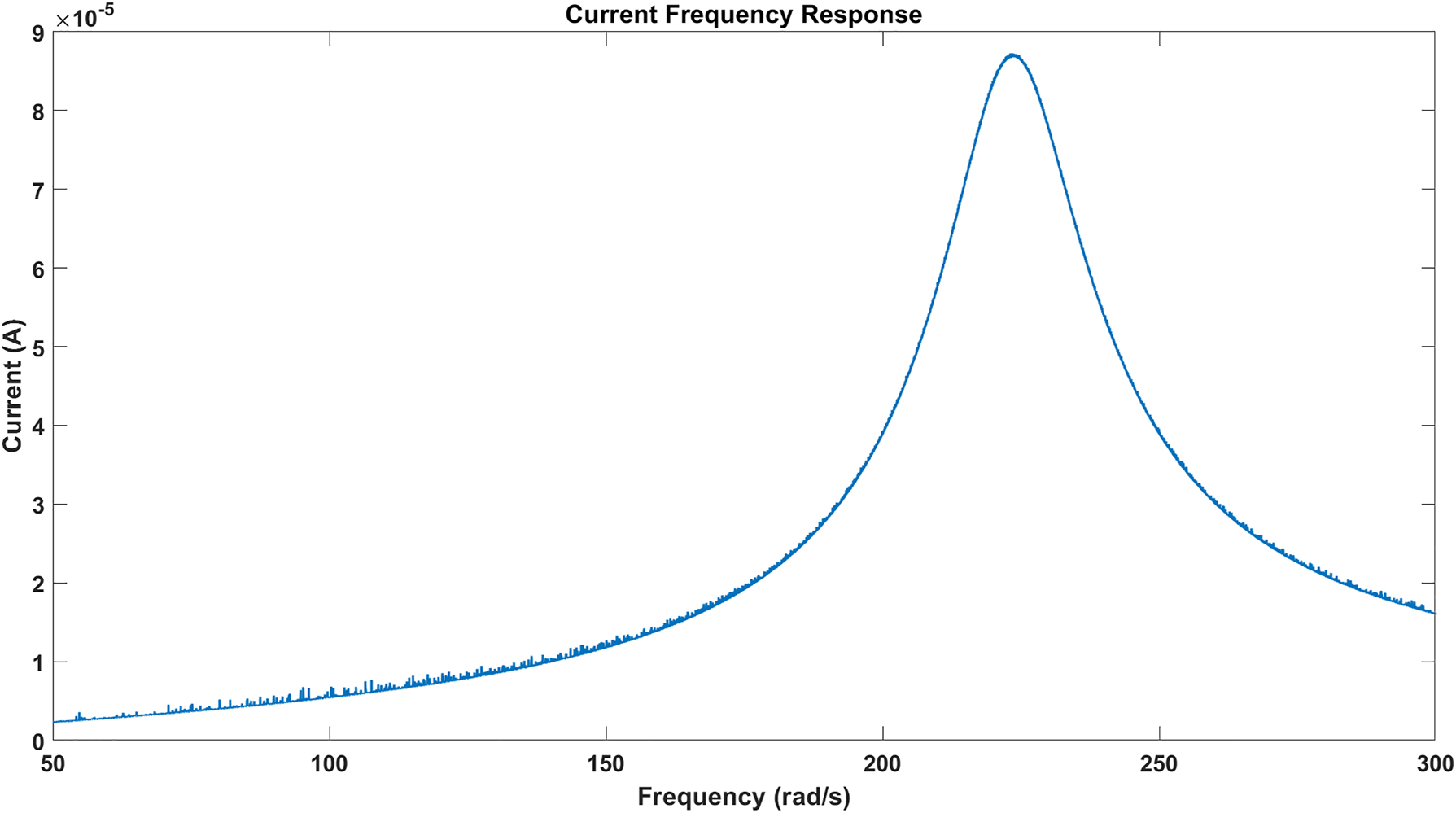
Current frequency response.
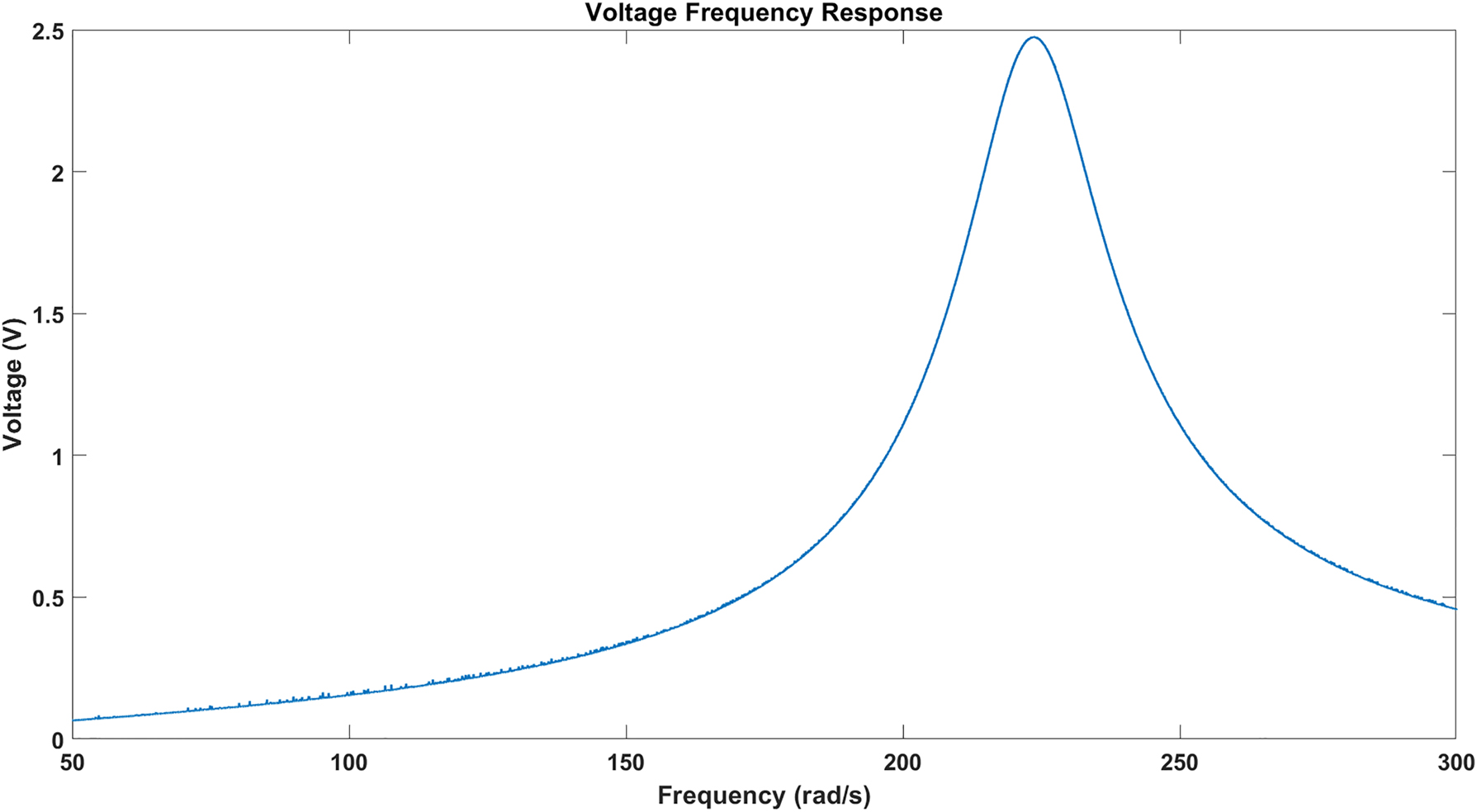
Voltage frequency response.
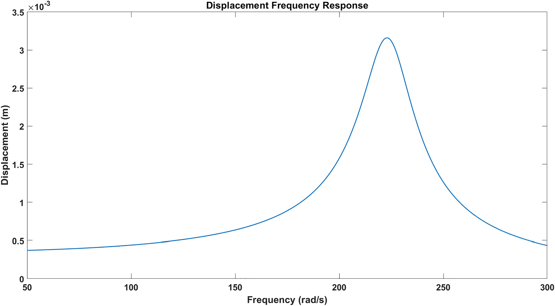
Displacement frequency response.
Note that in contrast to linear EVEH whose frequency response peaks at a different frequency in comparison to mechanical resonance frequency (Dezhara 2022b), the frequency response of the nonlinear one peaks at the linear mechanical resonance frequency.
4 Conclusions
We conclude that the homotopy method results in a more accurate response than other methods such as harmonic balance which assumes the response is simple harmonic and ignores higher harmonics. Plotting the frequency response after the optimum parameters design of EVEH is a good way to specify the resonance frequency of EVEH, and based on the numerical example of this paper this resonance frequency occurs at the linear mechanical resonance frequency. Note that in the case of linear EVEH at resonance mechanical frequency no power will deliver to the electrical load. However, in the case of nonlinear one maximum power is delivered to the load at the linear mechanical resonance frequency.
-
Author contributions: The author has accepted responsibility for the entire content of this submitted manuscript and approved submission.
-
Research funding: None declared.
-
Conflict of interest statement: The author declares no conflicts of interest regarding this article.
References
Aldawood, G., H. T. Nguyen, and H. Bardaweel. 2019. “High Power Density Spring-Assisted Nonlinear Electromagnetic Vibration Energy Harvester for Low Base-Accelerations.” Applied Energy 253: 113546. https://doi.org/10.1016/j.apenergy.2019.113546.Search in Google Scholar
Anjum, N., and J.-H. He. 2020. “Homotopy Perturbation Method for N/Mems Oscillators.” Mathematical Methods in the Applied Sciences. https://doi.org/10.1002/mma.6583.Search in Google Scholar
Bayat, M., I. Pakar, and L. Cveticanin. 2014. “Nonlinear Free Vibration of Systems with Inertia and Static Type Cubic Nonlinearities: An Analytical Approach.” Mechanism and Machine Theory 77: 50–8. https://doi.org/10.1016/j.mechmachtheory.2014.02.009.Search in Google Scholar
Bayat, M., M. Head, L. Cveticanin, and P. Ziehl. 2022. “Nonlinear Analysis of Two-Degree of Freedom System with Nonlinear Springs.” Mechanical Systems and Signal Processing 171: 108891. https://doi.org/10.1016/j.ymssp.2022.108891.Search in Google Scholar
Dezhara, A. 2022a. “The Efficiency of Linear Electromagnetic Vibration-Based Energy Harvester at Resistive, Capacitive and Inductive Loads.” Energy Harvesting and Systems 10 (1): 93–104. https://doi.org/10.1515/ehs-2022-0028.Search in Google Scholar
Dezhara, A. 2022b. “Frequency Response Locking of Electromagnetic Vibration-Based Energy Harvesters Using a Switch with Tuned Duty Cycle.” Energy Harvesting and Systems 9 (1): 83–96. https://doi.org/10.1515/ehs-2021-0057.Search in Google Scholar
Ganji, D. D., H. Tari, and M. B. Jooybari. 2007. “Variational Iteration Method and Homotopy Perturbation Method for Nonlinear Evolution Equations.” Computers and Mathematics with Applications 54 (7): 1018–27. https://doi.org/10.1016/j.camwa.2006.12.070.Search in Google Scholar
Ghadimi, M., and H. D. Kaliji. 2013. “Application of the Harmonic Balance Method on Nonlinear Equations.” World Applied Sciences Journal 22: 532–7.Search in Google Scholar
He, J.-H. 1999. “Homotopy Perturbation Technique.” Computer Methods in Applied Mechanics and Engineering 178 (3): 257–62. https://doi.org/10.1016/s0045-7825(99)00018-3.Search in Google Scholar
He, J.-H. 2000. “A Coupling Method of a Homotopy Technique and a Perturbation Technique for Non-Linear Problems.” International Journal of Non-Linear Mechanics 35: 37–43. https://doi.org/10.1016/s0020-7462(98)00085-7.Search in Google Scholar
He, J.-H. 2003. “Homotopy Perturbation Method: A New Nonlinear Analytical Technique.” Applied Mathematics and Computation 135 (1): 73–9. https://doi.org/10.1016/s0096-3003(01)00312-5.Search in Google Scholar
Kamaraj, A. K., S. F. Ali, and A. Arockiarajan. 2015. “Pizomahnetoelastic Broadband Energy Harveter: Nonlinear Modeling and Chracterization.” The European Physical Journal - Special Topics 224: 2803–22. https://doi.org/10.1140/epjst/e2015-02590-8.Search in Google Scholar
Kubba, A. E., and K. Jiang. 2014. “A Comprehensive Study on Technologies of Tyre Monitoring Systems and Possible Energy Solutions.” Sensors 14 (6): 10306–45. https://doi.org/10.3390/s140610306.Search in Google Scholar PubMed PubMed Central
Yu, D.-N., J.-H. He, and A. G. García. 2019. “Homotopy Perturbation Method with an Auxiliary Parameter for Nonlinear Oscillators.” Journal of Low Frequency Noise, Vibration and Active Control 38 (3–4): 1540–54, https://doi.org/10.1177/1461348418811028.Search in Google Scholar
© 2024 the author(s), published by De Gruyter, Berlin/Boston
This work is licensed under the Creative Commons Attribution 4.0 International License.
Articles in the same Issue
- Solar photovoltaic-integrated energy storage system with a power electronic interface for operating a brushless DC drive-coupled agricultural load
- Analysis of 1-year energy data of a 5 kW and a 122 kW rooftop photovoltaic installation in Dhaka
- Reviews
- Real yields and PVSYST simulations: comparative analysis based on four photovoltaic installations at Ibn Tofail University
- A comprehensive approach of evolving electric vehicles (EVs) to attribute “green self-generation” – a review
- Exploring the piezoelectric porous polymers for energy harvesting: a review
- A strategic review: the role of commercially available tools for planning, modelling, optimization, and performance measurement of photovoltaic systems
- Comparative assessment of high gain boost converters for renewable energy sources and electrical vehicle applications
- A review of green hydrogen production based on solar energy; techniques and methods
- A review of green hydrogen production by renewable resources
- A review of hydrogen production from bio-energy, technologies and assessments
- A systematic review of recent developments in IoT-based demand side management for PV power generation
- Research Articles
- Hybrid optimization strategy for water cooling system: enhancement of photovoltaic panels performance
- Solar energy harvesting-based built-in backpack charger
- A power source for E-devices based on green energy
- Theoretical and experimental investigation of electricity generation through footstep tiles
- Experimental investigations on heat transfer enhancement in a double pipe heat exchanger using hybrid nanofluids
- Comparative energy and exergy analysis of a CPV/T system based on linear Fresnel reflectors
- Investigating the effect of green composite back sheet materials on solar panel output voltage harvesting for better sustainable energy performance
- Electrical and thermal modeling of battery cell grouping for analyzing battery pack efficiency and temperature
- Intelligent techno-economical optimization with demand side management in microgrid using improved sandpiper optimization algorithm
- Investigation of KAPTON–PDMS triboelectric nanogenerator considering the edge-effect capacitor
- Design of a novel hybrid soft computing model for passive components selection in multiple load Zeta converter topologies of solar PV energy system
- A novel mechatronic absorber of vibration energy in the chimney
- An IoT-based intelligent smart energy monitoring system for solar PV power generation
- Large-scale green hydrogen production using alkaline water electrolysis based on seasonal solar radiation
- Evaluation of performances in DI Diesel engine with different split injection timings
- Optimized power flow management based on Harris Hawks optimization for an islanded DC microgrid
- Experimental investigation of heat transfer characteristics for a shell and tube heat exchanger
- Fuzzy induced controller for optimal power quality improvement with PVA connected UPQC
- Impact of using a predictive neural network of multi-term zenith angle function on energy management of solar-harvesting sensor nodes
- An analytical study of wireless power transmission system with metamaterials
- Hydrogen energy horizon: balancing opportunities and challenges
- Development of renewable energy-based power system for the irrigation support: case studies
- Maximum power point tracking techniques using improved incremental conductance and particle swarm optimizer for solar power generation systems
- Experimental and numerical study on energy harvesting performance thermoelectric generator applied to a screw compressor
- Study on the effectiveness of a solar cell with a holographic concentrator
- Non-transient optimum design of nonlinear electromagnetic vibration-based energy harvester using homotopy perturbation method
- Industrial gas turbine performance prediction and improvement – a case study
- An electric-field high energy harvester from medium or high voltage power line with parallel line
- FPGA based telecommand system for balloon-borne scientific payloads
- Improved design of advanced controller for a step up converter used in photovoltaic system
- Techno-economic assessment of battery storage with photovoltaics for maximum self-consumption
- Analysis of 1-year energy data of a 5 kW and a 122 kW rooftop photovoltaic installation in Dhaka
- Shading impact on the electricity generated by a photovoltaic installation using “Solar Shadow-Mask”
- Investigations on the performance of bottle blade overshot water wheel in very low head resources for pico hydropower
- Solar photovoltaic-integrated energy storage system with a power electronic interface for operating a brushless DC drive-coupled agricultural load
- Numerical investigation of smart material-based structures for vibration energy-harvesting applications
- A system-level study of indoor light energy harvesting integrating commercially available power management circuitry
- Enhancing the wireless power transfer system performance and output voltage of electric scooters
- Harvesting energy from a soldier's gait using the piezoelectric effect
- Study of technical means for heat generation, its application, flow control, and conversion of other types of energy into thermal energy
- Theoretical analysis of piezoceramic ultrasonic energy harvester applicable in biomedical implanted devices
- Corrigendum
- Corrigendum to: A numerical investigation of optimum angles for solar energy receivers in the eastern part of Algeria
- Special Issue: Recent Trends in Renewable Energy Conversion and Storage Materials for Hybrid Transportation Systems
- Typical fault prediction method for wind turbines based on an improved stacked autoencoder network
- Power data integrity verification method based on chameleon authentication tree algorithm and missing tendency value
- Fault diagnosis of automobile drive based on a novel deep neural network
- Research on the development and intelligent application of power environmental protection platform based on big data
- Diffusion induced thermal effect and stress in layered Li(Ni0.6Mn0.2Co0.2)O2 cathode materials for button lithium-ion battery electrode plates
- Improving power plant technology to increase energy efficiency of autonomous consumers using geothermal sources
- Energy-saving analysis of desalination equipment based on a machine-learning sequence modeling