Real yields and PVSYST simulations: comparative analysis based on four photovoltaic installations at Ibn Tofail University
-
Oumaima Ait Omar
 ,
Hassan EL Fadil
,
Hassan EL Fadil

Abstract
Since the PVSYST simulator is the most well-known software among researchers and PV experts, we chose to compare its results to those of the manual method. Thus, the objective of the article was to obtain the degree of similarity between the results of the PVSYST simulation and the manual calculation of the same parameters, based on the study of the photovoltaic systems of the University Ibn Tofail. Those installations are installed in the Faculty of Letters, Science, the Presidency and CFC. The later used in our study, have different parameters. Hence, to collect these parameters and their distinct data we used multiple sources. The datasheets of each components of the PV system contains the parameters that distinguish the devices therefore it was mandatory to look for that information, since it will facilitate our study. The meteorological database PVGIS, was our reference for the temperature and irradiation data. What’s more is the PVSYST software that helps in the simulation of the PV system and thus having a detailed report with massive information. All this collection of data was aiming to help us comparing the results of yields and other parameters by manual calculation versus simulation in PVSYST. Morocco has demonstrated a strong commitment to combat climate change by embracing renewable energy, particularly photovoltaic systems. In this pursuit, universities like Ibn Tofail University (UIT) play a crucial role in addressing climate challenges and developing research solutions for mitigation. UIT actively participates in projects related to environmental protection and sustainable development, contributing to Morocco’s growth and higher education advancement. As part of its efforts, UIT has been involved in implementing sustainable green projects and promoting renewable energy technologies. A specific study at UIT aimed to compare PVSYST simulation results with manual calculations for four PV systems on campus, considering parameters such as orientation, electrical installation, and panel types. The International Energy Agency (IEA) Photovoltaic Systems Program has established standards and a key concept, the yield factor, measuring the net energy production over a facility’s lifetime compared to the energy used for construction, operation, and supply. By evaluating the accuracy and efficiency of PVSYST, researchers sought to advance the use of PV systems and contribute to Morocco’s renewable energy goals. Such research not only aids in the progression of renewable energy technology but also aligns with Morocco’s vision for sustainable development and environmental protection.
1 Introduction
Energy is often simply defined as the ability to do work or generate heat. Human beings con-sume energy in almost every aspect of life, and the source of energy varies with the degree of human civilization. In early human history, humans depended on the muscular strength of the human body, the energy of animals, the sun, water and air. However, with the discovery of fire, people began to use biomass as an energy source. Energy from the sun, wind, biomass, hydroelectricity, and geothermal energy are called renewable energy sources that naturally renew themselves in a short period of time. As human civilization progressed, coal was dis-covered and it largely replaced biomass, especially in industrialized countries. The discovery of oil and natural gas is significantly displacing coal, especially in developed countries. Coal, uranium, oil and natural gas are called non-renewable energy sources because they are de-pletable and take a long time to form (What is Energy). There is empirical evidence for links between energy use and population growth, and between energy use and economic growth.
The relationship between energy consumption and economic growth in China, India, and G7 countries from 1965 to 2017 is studied by applying multi-spatial fusion cross-mapping (CCM). For research purposes, the two sets of data, total energy consumption (EC) per capita in million tons of oil equivalent and real gross domestic product (GDP) calculated at constant prices in 2010 are from BP Statistical Yearbook of World Energy and World Development Indicators (WDI). A multi-spatial aggregated cross-mapping (CCM) analysis of the collected data revealed positive correlations between energy consumption and economic growth in the United States (US), Japan, Italy and Canada, China and India.
Photovoltaic self-consumption, energy efficiency and electric vehicles are topics of particular interest to ITU. Projects on these topics include green energy and the environment, photovoltaic systems. Several software programs optimize the simulation results of photovoltaic systems, PVSYST software is one of the most commonly used (El Mokhi et al. 2022). Therefore, efficiency and accuracy are keywords that every software user hopes to obtain, especially when the richness of the software confuses them. Morocco’s commitment to international efforts to combat climate change has been translated over time into concrete actions and plans in different sectors (Choukai et al. 2022). Therefore, efficiency and accuracy are keywords that every software user hopes to obtain, especially when the richness of the software confuses them. Morocco’s commitment to international efforts to combat climate change has been translated over time into concrete actions and plans in different sectors (Ait Errouhi et al. 2022). To implement the Royal Vision, Moroccan universities, especially Ibn Tofail University, are aware of climate change issues, especially since researchers at these universities have sounded the alarm and have the mechanisms and resources to assess the state of the Earth and in the context of climate change From the perspective of providing solutions for adaptation and mitigation, Ibn Tofail University (UIT) is committed to providing solutions through the development of scientific research and the accompanying public policy deadlines (Author Anonymous). UIT fulfills its mission to contribute to Morocco’s sustainable development, higher education advancement and economic growth by adopting and implementing several promising projects in the fields of development and environment. The University strives to further develop its contribution to research and its relationships with various stakeholders. UIT is firmly committed to environmental protection and actively participates in the implementation of sustainable green projects (Présentation de l’UIT).
The parameters describing energy photovoltaic systems and their components were developed by the International Energy Agency (IEA) Photovoltaic Systems Program and described in IEC standards (Ekeocha, Penzin, and Ogbuabor 2020). In short, the general definition of a power plant production factor describes how much of the energy produced during a power plant’s operation covers the energy used to build the plant.
Since the PVSYST simulator is the most famous software among researchers and PV experts, we decided to compare its results with those of manual methods. Therefore, the aim of this paper is to determine the degree of similarity between the PVSYST simulation results and the manual calculation results for the same parameters, based on a study of photovoltaic systems at the University of Ibn Tofail (Chandrika et al. 2020). Four photovoltaic systems were installed at the later university. These installations are installed in the Faculties of Letters, Science, President and CFC. The ones used later in our study have different parameters (orientation, electrical installation, type of photovoltaic panels …). Therefore, in order to collect these parameters and their various data, we used several sources (Chioncel et al. 2010; Kasim, Hussain, and Abed 2019). The data sheet for each component of a photovoltaic system contains parameters that differentiate the device, so it is imperative to look up this information as it will aid our research. The meteorological database PVGIS is our reference for obtaining temperature and sunshine data (Verma, Yadav, and Sengar 2021). In addition, PVSYST software facilitates the simulation of photovoltaic systems, thereby providing detailed reports with a wealth of information. All this data collection should help us compare the results of yield and other parameters with simulations in PVSYST through manual calculations (Mermoud and Wittmer 2014).
2 Detailed design and methodology
2.1 Collection of data
We will first determine the energy produced from E ac and E dc for each installation. To obtain the E ac and E dc energies, we had to retrieve them from the Solar–Log or Solar–Web™ website, put them in an Excel file and thus, calculate the average which will be used in the calculations.
2.1.1 Faculty Letters
The average E dc = 227.706 and E ac = 222.876 are calculated from the values of 03, 27, 28 June 2020 and 03, 10 June 2020 for the summer. For winter, the average E dc = 185.59 and E ac = 181.326 are calculated from the values of 11, 12, 30 January 2020 and 01, 03 February 2020 (literature university) Table 1.
E ac and E dc of 4 installations in summer and winter.
| FL (Letters Faculty) | FS (Sciences Faulty) | Presidency | CEC | ||
|---|---|---|---|---|---|
| E dc (kWh) | 227.70 | 274.42 | 106.96 | 220.16 | |
| Summer | E ac (kWh) | 222.87 | 263.03 | 102.90 | 216.20 |
| System size (kWp) | 46.8 | 60 | 21.06 | 34.56 | |
| E dc (kWh) | 185.59 | 219.45 | 84.95 | 121.82 | |
| Winter | E ac (kWh) | 181.32 | 210.70 | 81.83 | 119.82 |
| System size (kWp) | 46.8 | 60 | 21.06 | 34.56 |
2.1.2 Faculty Sciences
The average E dc = 274.4225 and E ac = 263.03 are calculated from the values of 01, 19 July 2021 and 05, 23 June 2021 for the summer. Regarding the winter, the average E dc = 219.4525 and E ac = 210.7075 are calculated from the values of 11, 12 January 2021 and 01, 03 February 2021 (Faculty of Science) Table 1.
2.1.3 Presidency
The average E dc = 106.96 and E ac = 102.8966667 are calculated from the values of 07, 12, 11 July 2021 and 05, 28, 29 June 2021 for the summer. For winter, the average E dc = 84.95833333 and E ac = 81.83666667 are calculated from the values of 04, 12 January 2021 and 10, 14, 23 February 2021 (Presidency) Table 1.
2.1.4 Center for continuing education
The average E dc = 220.1575 and E ac = 216.2 are calculated from the values of 07, 20 July 2021 and 01, 05 June 2021 for the summer. For the winter, the average E dc = 121.825 and E ac = 119.825 are calculated from the values of 03, 18 January 2021 and 15, 16 February 2021 (Center of Continuing Education CFC) Table 1.
Then, we will have to extract the irradiation of the two months January and February of the winter season, and June and July of the summer season. PVGIS is a web site containing the meteorological database such as irradiation and temperature. Choosing the location and month of study and integrating it into PVGIS is essential to have the exact irradiation values since they change depending on the geographical location and month. The following figures and tables represent the irradiation of the months January, February, June, and July.
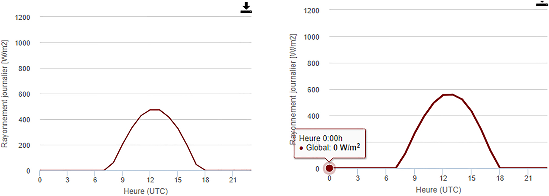
The curves in Figure 1 represent the daily irradiation pattern of the two months January and February of the winter season where the irradiation decreases due to climatic conditions.
The average of the daily values for the month of February equals 342.22 W/m2, and for January, it equals 295.781 W/m2 (Table 2).
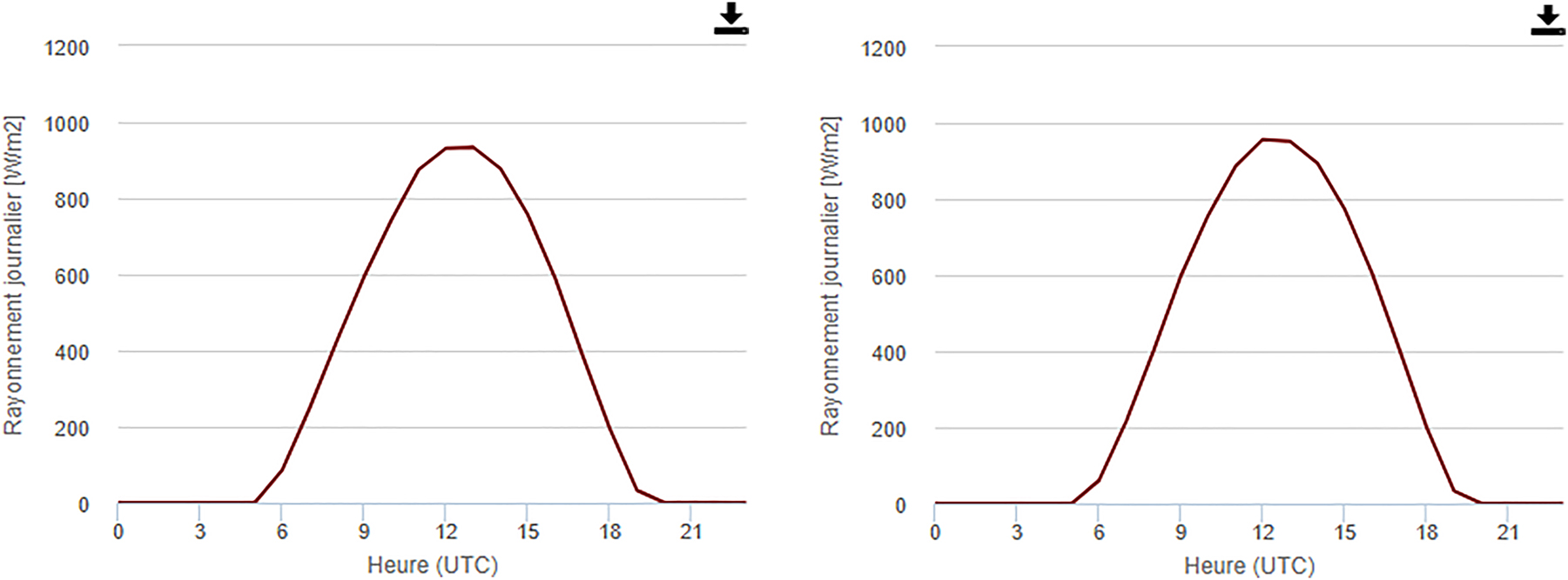
The curves in Figure 2 represent the daily irradiation of the two months June and July of the summer season where we notice a considerable increase.
The average of the daily values for June equals 547.81 W/m2, and for July, it is 552.67 W/m2 (Table 3).
Irradiation of February and January-PVGIS meteorological database.
Irradiation: January and February-PVGIS meteorological database.
| January W/m2 | February W/m2 | |
|---|---|---|
| 59.83 | 111.44 | |
| 204.9 | 265.85 | |
| 331.87 | 394.56 | |
| 427.42 | 495.58 | |
| 472.92 | 554.94 | |
| 472.93 | 558.90 | |
| 417.65 | 522.49 | |
| 328.55 | 432.08 | |
| 196.7 | 295.62 | |
| 45.04 | 132.3 | |
| – | 0.66 | |
| Average irradiation W/m 2 | 295.78 | 342.22 |
-
Bold values represent the daily irradiation in W/m2.
Irradiation of July and June-PVGIS meteorological database.
Irradiation: June and July-PVGIS meteorological database.
| June W/m2 | July W/m2 | ||
|---|---|---|---|
| 85.29 | 60.60 | ||
| 247.50 | 217.03 | ||
| 424.43 | 401.48 | ||
| 593.60 | 598.86 | ||
| 742.47 | 757.92 | ||
| 875.16 | 886.27 | ||
| 931.25 | 956.86 | ||
| 933.49 | 951.70 | ||
| 877.74 | 893.41 | ||
| 755.76 | 772.21 | ||
| 588.96 | 604.67 | ||
| 387.17 | 404.41 | ||
| 194.21 | 199.23 | ||
| 32.34 | 32.73 | ||
| Average irradiation W/m2 | 547.81 | 552.67 | |
A third step consists in listing the components of each photovoltaic installation. The orientation and inclination of each system are essential for the simulation of the pre-existing systems. The following table summarizes the components, their types, the number of modules for each installation and the installed power (Table 4).
The components of each installation.
| Data | Faculty Letters | Sciences Faculty | Presidency | CEC |
|---|---|---|---|---|
| Fabricant | JA SOLAR | JINKO SOLAR | JINKO SOLAR | BISOL |
| Type de PV | JAM60S01-315Wp | EAGLE DUAL 60 280Wc | EAGLE 60 270Wc | BISOL XL SERIES |
| Number of modules | 156 | 216 | 78 | 108 |
| Field power | 46.8 | 60.48 | 21.06 | 34.56 |
| Type of inverter | SUN2000-20KTL | SYMO 20.0-3-M | SYMO 20.0-3-M | DELTA ENERGY RPIM30A |
| Power of inverter kWc | 20 | 20 | 20 | 30 |
| Inverter efficiency | 98.65 % | 98.10 % | 98.10 % | 98.50 % |
| Angle | 15 | 13 | 15 | 15 |
| PV power rating (kWp) | 0.315 | 0.28 | 0.27 | 0.32 |
| Power kWp under field | (17 modules/4 chaînes) 21.42 | (18 modules/12 chaînes) 60.48 | (20 modules/2 chaînes) 10.8 | – |
| Area m2 | 111 | 353.54 | 65.47 | – |
| Power kWp under field | (22 modules/4 chaînes) 27.72 | – | (19 modules/2 chaînes) 10.26 | |
| Area m2 | 143.89 | – | 62.1984 | 210.41 |
| Orientation | 158 | −152 | −150 | −99 |
After the collection of data, we will proceed to evaluate PVSYST by comparing the results of two different methods:
Manuel method
Simulated method
2.2 Manuel method
2.2.1 Equation
We will calculate some parameters that we will use in the comparison. The system energy produced is divided into 3 types: reference energy, final energy produced after passing through the inverter and the energy of the PV system.
The energy produced by the PV system Y a is defined by E dc divided by the rated power of the system (Kasim, Hussain, and Abed 2019). The equation is written as follows:
E dc is the direct current energy (kWh).
As for the final energy Y f, it is defined by E ac divided by the PV system power. Y f represents the time during which the system operates in its rated power in hours or kWh/kW (Kasim, Hussain, and Abed 2019).
E ac represents the energy of the alternating current (kWh).
The reference energy is defined by dividing the global irradiation by the reference irradiation which equals: 1 kW/m2.
System and PV field losses:
L a: the collection losses: caused by obscuration, temperature rise, mismatching, dust covering the modules as well as the losses of the energy conducted in the PV modules (Kasim, Hussain, and Abed 2019).
L s: system losses caused by the inverter, conduction and losses of passive circuits (Kasim, Hussain, and Abed 2019).
The yield of a Photovoltaic installation is divided into 3 main parts:
The yield of the photovoltaic modules which is calculated as follows:
System performance:
Inverter efficiency:
The performance index, as its name suggests, is a parameter that determines the performance of the photovoltaic field. These values are between 70 % and 90 % and decrease by 1 % every year. The more losses you have, like dirt losses, wiring losses, component failure, or inverter losses, the lower your performance index will be (Verma, Yadav, and Sengar 2021).
CF is a method to evaluate the energy produced by the PV array.
2.2.2 Results
The following tables contain the calculation results of the parameters for the period of June/July (summer) and January/February (winter) Tables 5–8.
Calculation results of the FL parameters.
| F Letters | |||
|---|---|---|---|
| Winter | Summer | ||
| System yield | Array yield (Y a) | 3.96 | 4.86 |
| Finale yield (Y f) | 3.87 | 4.76 | |
| Reference yield (Y r) | 4.79 | 7.6 | |
| Array loss (L a) | 0.82 | 2.73 | |
| System energy loss (L s) | 0.09 | 0.10 | |
| PV solar array efficiency | 15.17 | 11.74 | |
| A (m2) | 255.08 | 255.08 | |
| System efficiency | 14.82 | 11.43 | |
| The inventer efficiency | 97.70 | 97.87 | |
| Performance ratio | 81 % | 63 % | |
| Capacity factor | 0.00044 | 0.00054 | |
Calculation results of the FS parameters.
| F Sciences | |||
|---|---|---|---|
| Winter | Summer | ||
| System yield | Array yield (Y a) | 3.62 | 4.53 |
| Finale yield (Y f) | 3.48 | 4.34 | |
| Reference yield (Y r) | 3.82 | 7.70 | |
| Array loss (L a) | 0.19 | 3.16 | |
| System energy loss (L s) | 0.14 | 0.18 | |
| PV solar array efficiency | 16.21 | 10.07 | |
| A (m2) | 353.54 | 353.54 | |
| System efficiency | 15.56 | 9.65 | |
| The inventer efficiency | 96.01 | 95.84 | |
| Performance ratio | 91 % | 56 % | |
| Capacity factor | 0.00039 | 0.00049 | |
Results of the calculation of the Presidency’s parameters.
| Presidency | |||
|---|---|---|---|
| Winter | Summer | ||
| System yield | Array yield (Y a) | 4.03 | 5.07 |
| Finale yield (Y f) | 3.88 | 4.88 | |
| Reference yield (Y r) | 4.78 | 7.60 | |
| Array loss (L a) | 0.75 | 2.52 | |
| System energy loss (L s) | 0.14 | 0.19 | |
| PV solar array efficiency | 13.89 | 11.02 | |
| A (m2) | 127.67 | 127.67 | |
| System efficiency | 13.38 | 10.60 | |
| The inventer efficiency | 96.32 | 96.20 | |
| Performance ratio | 81 % | 64 % | |
| Capacity factor | 0.00044 | 0.00055 | |
CFC parameter calculation results System yield.
| Centre de formation continue CEC | |||
|---|---|---|---|
| Winter | Summer | ||
| System yield | Array yield (Y a) | 3.52 | 6.37 |
| Finale yield (Y f) | 3.46 | 6.25 | |
| Reference yield (Y r) | 3.82 | 7.70 | |
| Array loss (L a) | 0.30 | 1.33 | |
| System energy loss (L s) | 0.06 | 0.11 | |
| PV solar array efficiency | 15.12 | 13.58 | |
| A (m2) | 210.41 | 210.41 | |
| System efficiency | 14.85 | 13.33 | |
| The inventer efficiency | 98.19 | 98.20 | |
| Performance ratio | 90 % | 81 % | |
| Capacity factor | 0.00039 | 0.00071 | |
2.3 Simulation method
2.3.1 PVSYST simulation
When using software, one always looks for an optimal result and minimum margin of error for the obtained results. PVSYST facilitates the task of dimensioning photovoltaic installations and allows to obtain various information such as energy production, necessary surface, and annual energy production (Chandrika et al. 2020).
To simulate the 4 photovoltaic installations, we need to:
First, choose the irradiation and temperature from the PVGIS weather database (Figure 3).
Second, the choice of tilts and orientations differ from one geographical location to another (Figure 4).
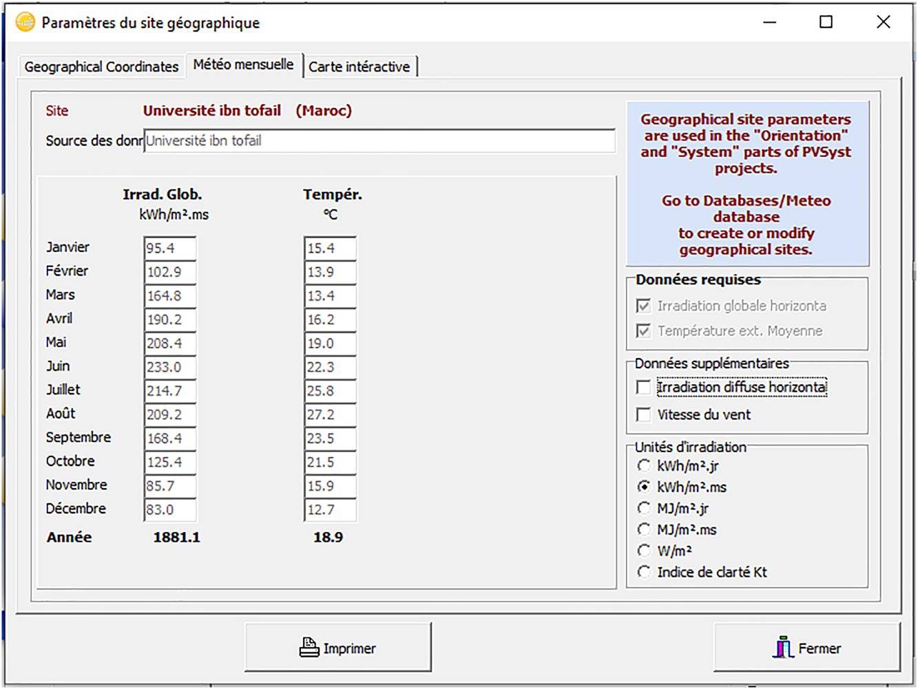
Geographic parameters of the site.
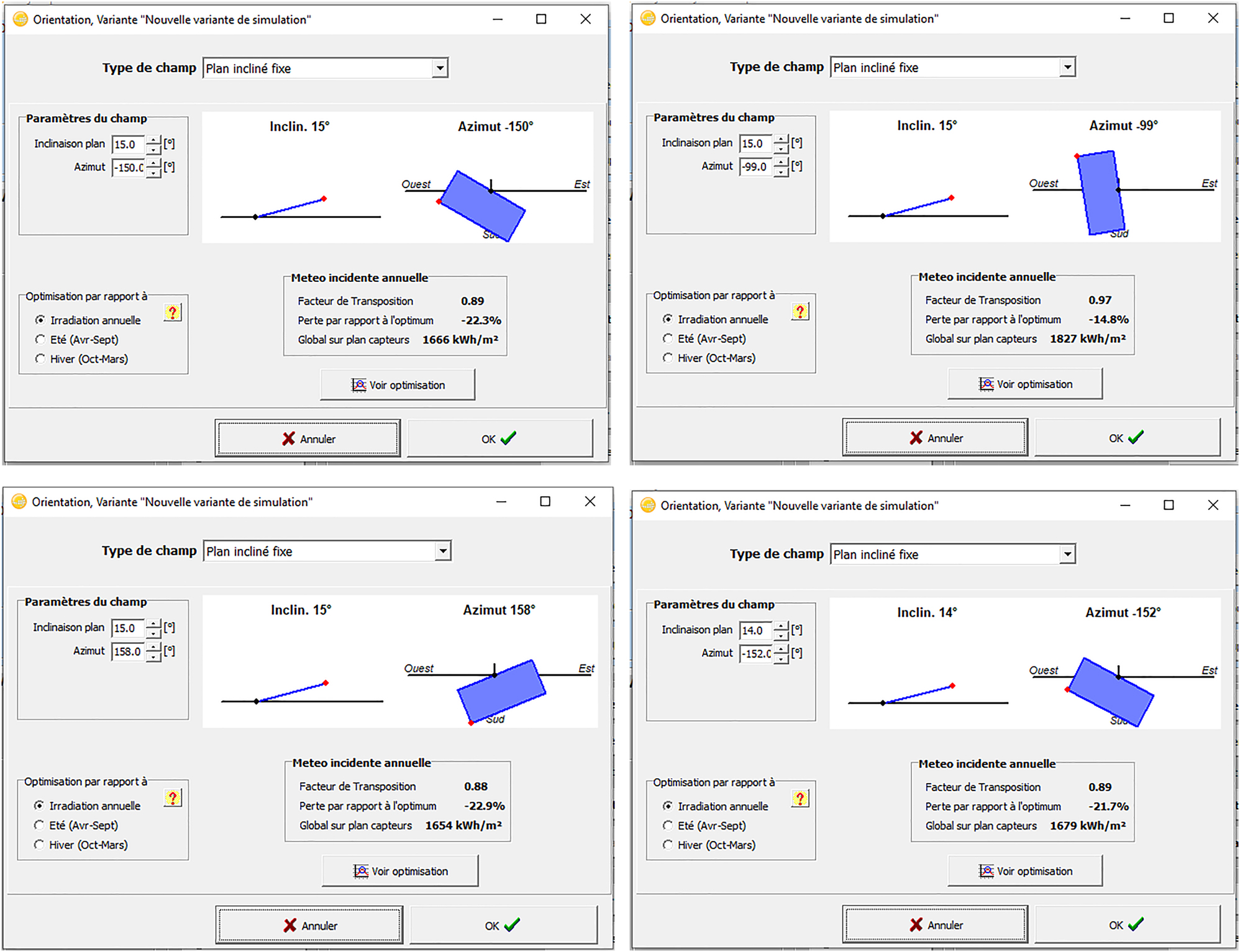
Orientations.
Third, the characteristics of each PV system (inverters, PV module type …) are entered into the software.
Concerning the installations of the Faculty of Letters (Figures 5 and 6) (power 46.8 kW and 156 number of modules), and for the Presidency (Figures 9 and 10) of the University Ibn Tofail (power 21.06 kW and 78 number of modules) their simulation was in the form of sub-fields contrary to the CFC (Figure 8) (power 34.56 kW to the number 108 modules) and faculty of Sciences (Figure 7) (power 60.48 kW and 216 number of modules) which constitutes a single field (Figures 8 –10).
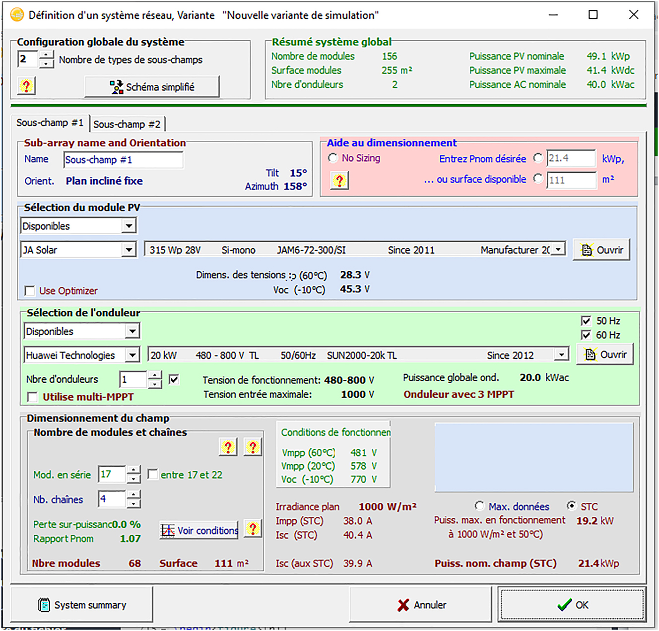
PVSYST project design of the F. Letter.
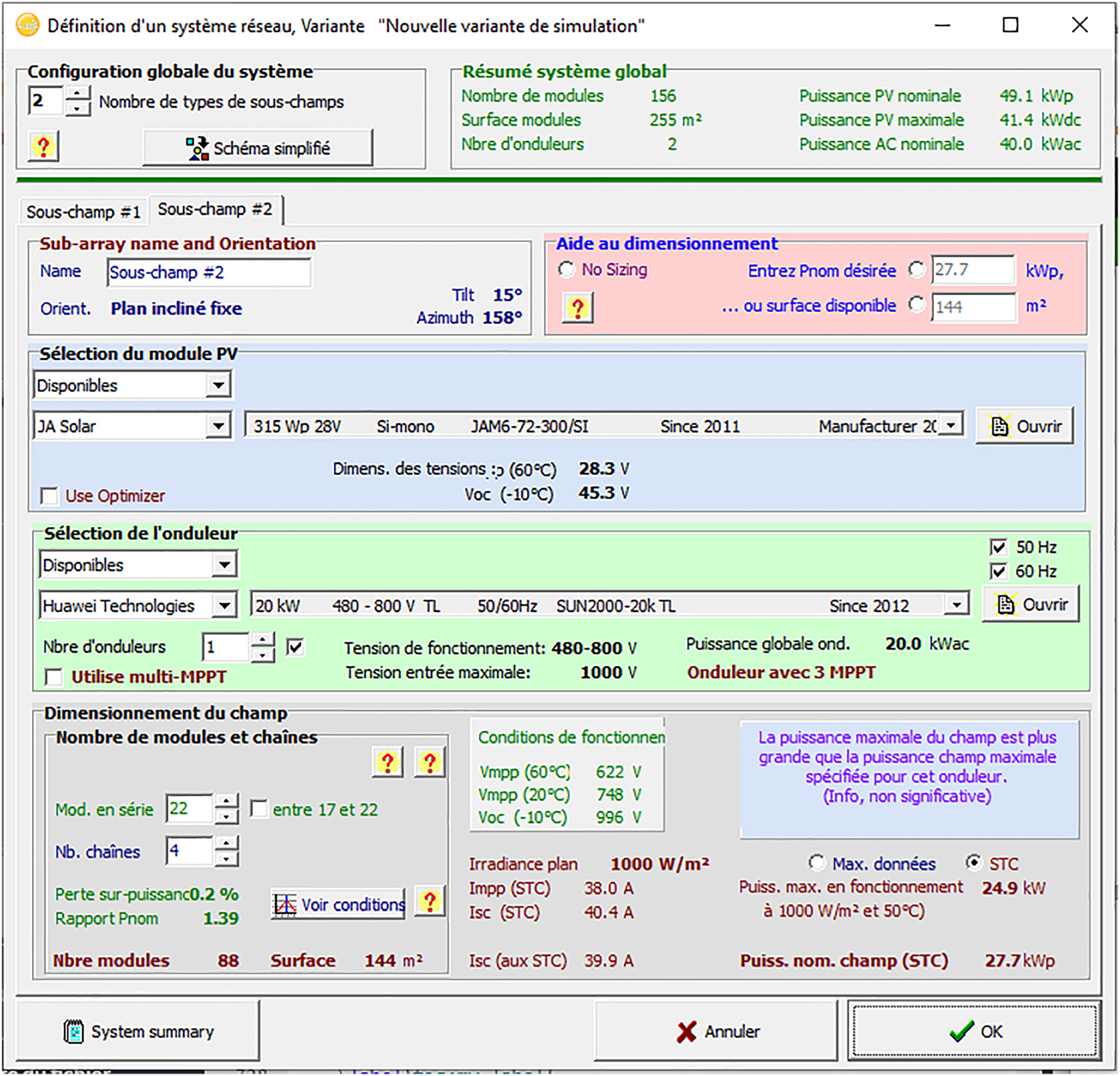
PVSYST project design the F. Letter.
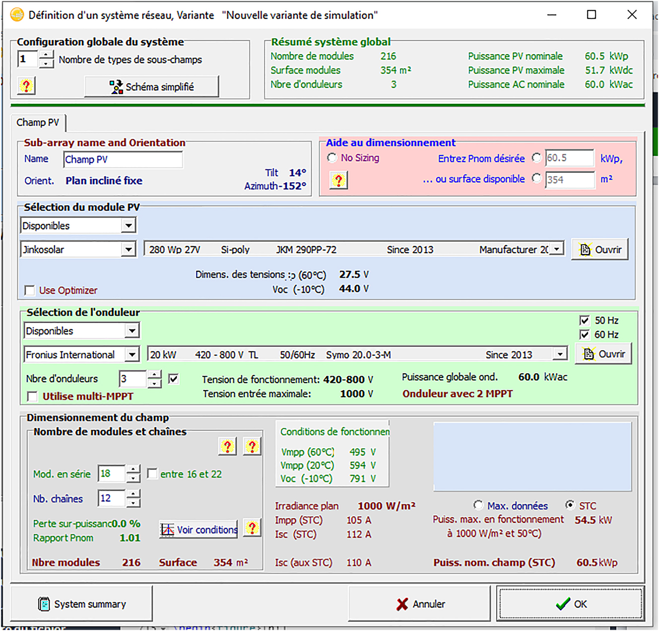
PVSYST project design of the Science Faculty.

PVSYST project design of the CFC.

PVSYST project design of the Presidency.
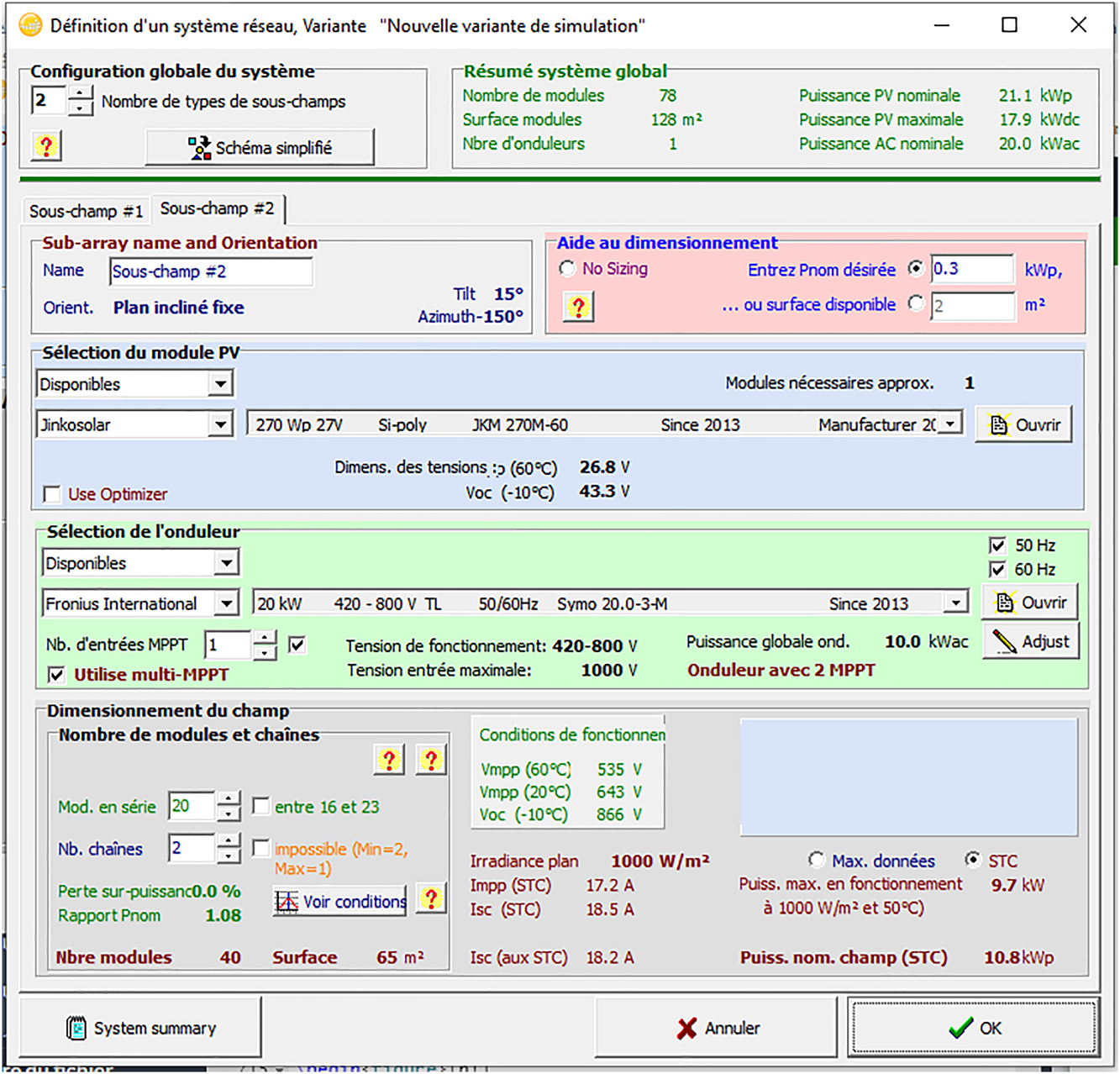
PVSYST project design of the Presidency.
2.3.2 Results of PVSYST simulation
The following figures determine 4 parameters which are: the performance index, the collection and system losses and the useful energy produced.
After the simulation of the installation of the Faculty of Letters, the normalized production (per kWp Installed) equal to 49.1 kWp does not differ strongly from the real value which equals 46.8 kWp. The performance index equals 0.854 considering all the months of the year (Figure 11).
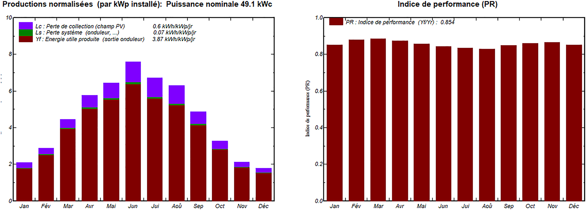
Nominal power et PR of Letters Faculty.
After the simulation of the installation of the Faculty of Science, the normalized production (per kWp Installed) equal to 60.5 kWp does not differ strongly from the real value which equals 60.48 kWp. The performance index equals 0.848 considering all the months of the year (Figure 12).

Simulation PVSYST nominal power et PR of Science Faculty.
After the simulation of the installation of the Presidency, the normalized production (per kWp Installed) equal to 21.06 kWp equals the real value. The performance index equals 0.850 considering all the months of the year (Figure 13).
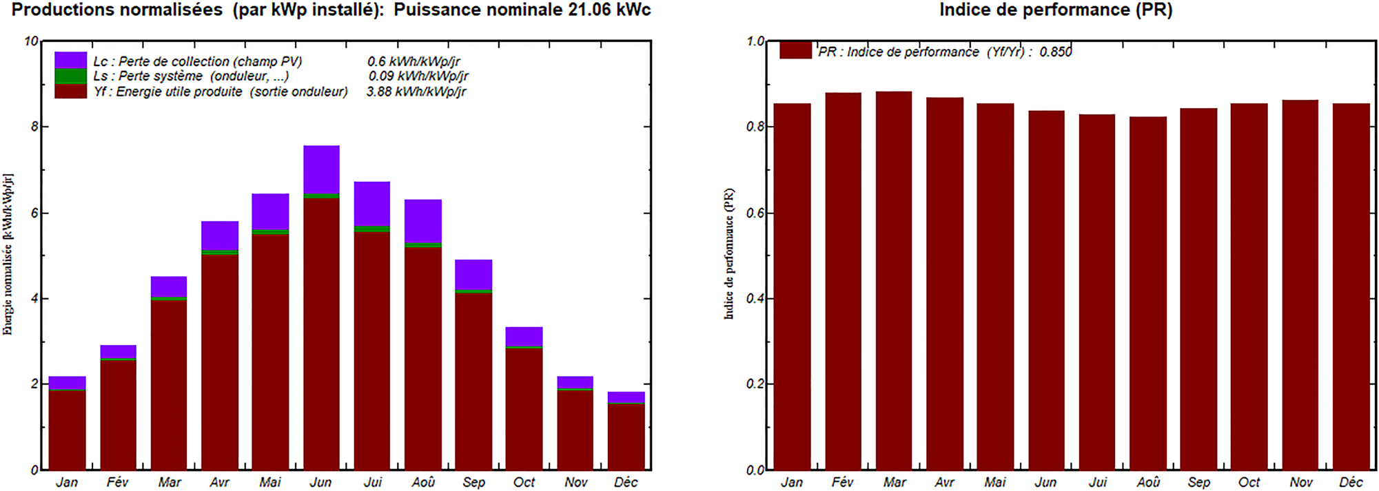
Simulation PVSYST nominal power et PR of the Presidency.
After the simulation of the CFC installation, the normalized production (per kWp Installed) equal to 34.6 kWp does not differ strongly from the real value which equals 34.56 kWp. The performance index equals 0.848 considering all the months of the year (Figure 14).
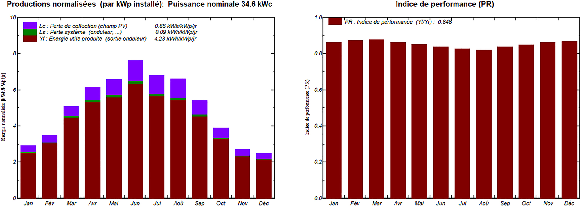
Simulation PVSYST nominal power et PR of the CFC.
The following diagrams summarize the different losses of the system such as the losses of inverters and cables to finally determine the value of energy injected into the network:
The nominal field energy (according to STC) of the first simulation of the Faculty of Letters is equal to 77.5 MWh/year which gives a value of energy injected into the grid of 69.4 MWh/year after losses at the irradiation levels, camp temperature, module quality as well as cable and inverter losses (Figure 15).
The nominal field energy (according to STC) of the first simulation of the Faculty of Science equals 97.2 MWh/year which gives a value of energy injected into the grid of 86.1 MWh/year after losses at irradiation levels, camp temperature, module quality as well as cable and in-verter losses (Figure 16).
The energy injected into the grid equals 29.6 MWh/year after losses at irradiation levels (−0.3 %), field temperature (−7.7 %), module quality (+0.7 %) as well as cable and inverter losses (Figure 17).
The energy injected into the grid equals 54.5MWh/year after losses at irradiation levels (−2.1 %), field temperature (−8.1 %), module quality (+0.7 %) as well as cable and inverter losses (Figure 18).
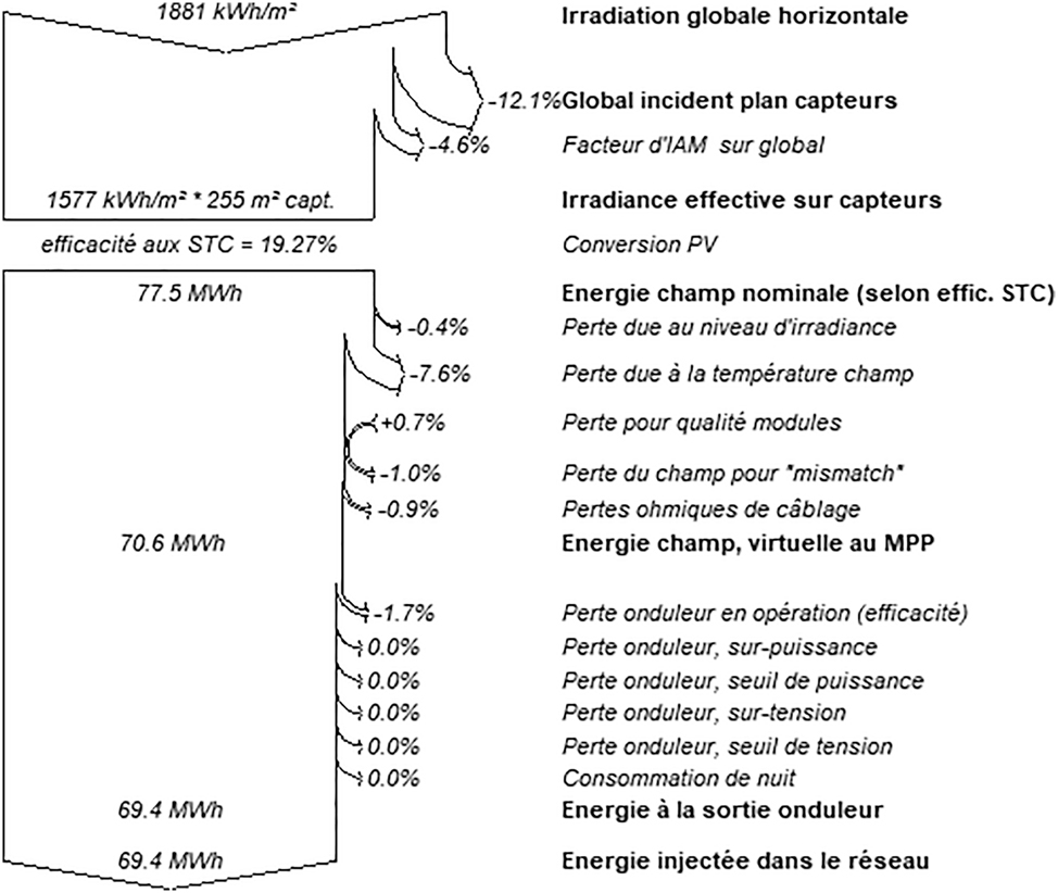
Loss diagram: Faculty of Letters.
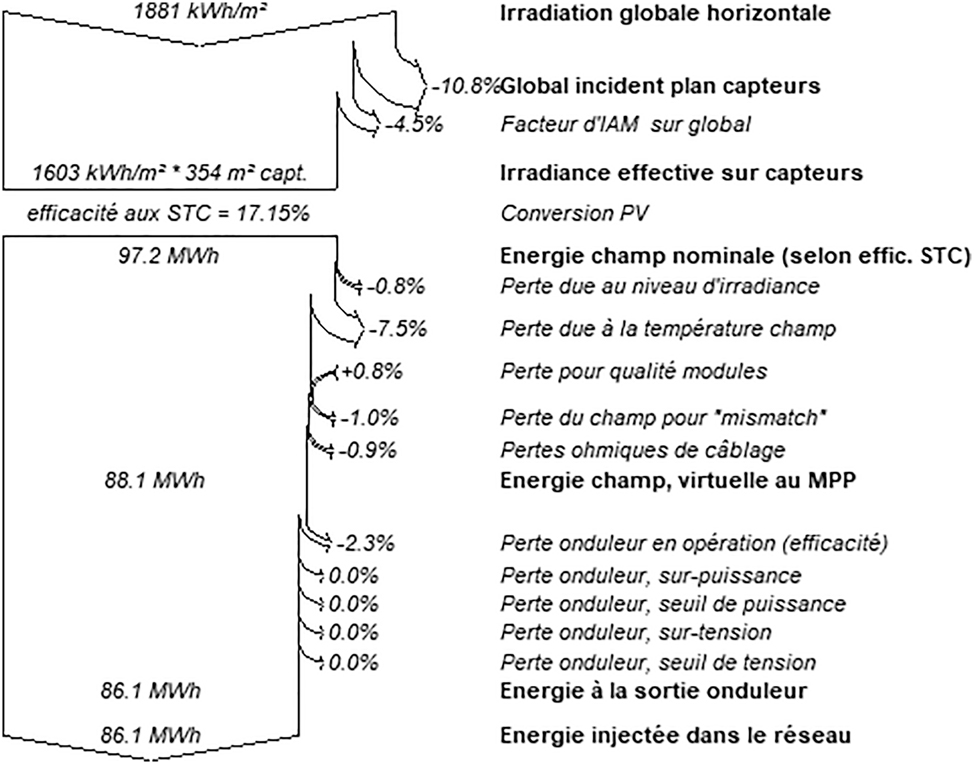
Loss diagram: Faculty of Science.
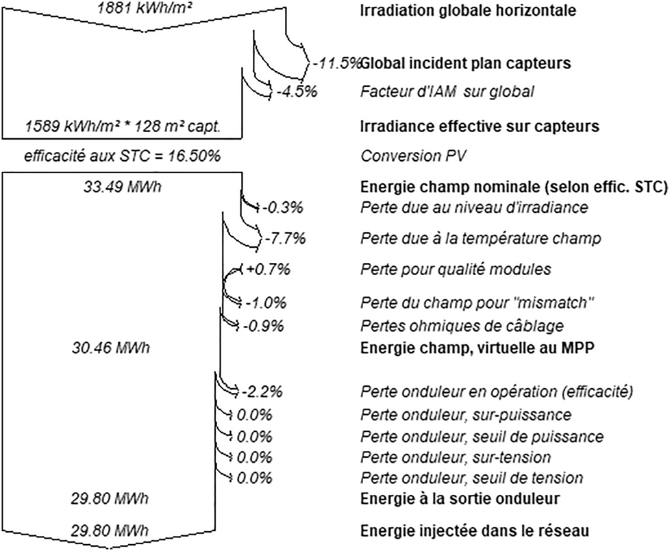
Loss diagram: Presidency.
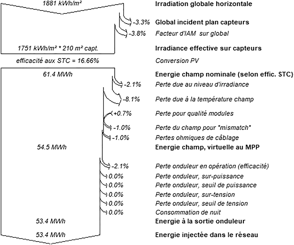
Loss diagram: CFC.
2.4 SImulation and calculation results
The following tables summarize the results obtained for the calculations and simulations of the 4 installations (Tables 9 –16):
The sum of the calculated index PR gives a value of PR = 72 % and the value of the simulation PVSYST PR = 85.4 %, so we have a gap of 13.4 % (F Letters).
Calculated parameters: F. Letters.
| Calculation of parameters using PVGIS data | ||
|---|---|---|
| Winter | Summer | |
| Module loss | 0.82 | 2.73 |
| System loss | 0.091 | 0.103 |
| Efficiency pv module | 15.17 | 11.74 |
| System efficiency | 14.82 | 11.49 |
| Inverter efficiency | 97.70 | 97.87 |
| Performance index | 0.81 | 0.63 |
| CF | 0.00044 | 0.00054 |
Simulated parameters: F. Letters.
| PVSYST simulation with PVGIS data | |
|---|---|
| Module quality loss | −0.008 |
| Energy produced | 69.37 MWh/year |
| PR index | 0.854 |
| Final yield | 3.87 kWh/kp/day |
| L c | 0.60 kWh/kWp/day |
| L s | 0.07 kWh/kW/day |
| Inverter loss in operation | −1.70 % |
| Efficiency at STC | 19.27 % |
| Global irradiation H (kWh/m2) | 1881 |
| Incidence angle modified | −4.60 % |
| GI sensor plane | −12.10 % |
-
The sum of the calculated index PR gives a value of PR = 73.5 % and the value of the PVSYST simulation PR = 84.8 % hence a difference of 11.3 %.
Calculated parameters: F. Sciences.
| Calculation of parameters using PVGIS data | ||
|---|---|---|
| Winter | Summer | |
| Module loss | 0.199 | 3.16 |
| System loss | 0.144 | 0.188 |
| Efficiency pv module | 16.21 | 10.07 |
| System efficiency | 15.56 | 9.65 |
| Inverter efficiency | 96.01 | 95.84 |
| Performance index | 0.91 | 0.56 |
| CF | 0.00039 | 0.00049 |
Simulated parameters: F. Sciences.
| PVSYST simulation with PVGIS data | |
|---|---|
| Module quality loss | −0.008 |
| Energy produced | 86.06 MWh/year |
| PR index | 0.848 |
| Final yield | 3.9 kWh/kp/day |
| L c | 0.61 kWh/kWp/day |
| L s | 0.09 kWh/kW/day |
| Inverter loss in operation | −2.30 % |
| Efficiency at STC | 17.15 % |
| Global irradiation H (kWh/m2) | 1881 |
| Incidence angle modified | −4.50 % |
| GI sensor plane | −10.80 % |
-
The sum of the calculated index PR gives a value of PR = 72.5 % and the value of the simulation PVSYST PR = 85 % which is a difference of 12.5 %.
Calculated parameters: Presidency.
| Calculation of parameters using PVGIS data | ||
|---|---|---|
| Winter | Summer | |
| Module loss | 0.75 | 2.52 |
| System loss | 0.14 | 0.19 |
| Efficiency pv module | 13.89 | 11.02 |
| System efficiency | 13.38 | 10.60 |
| Inverter efficiency | 96.32 | 96.20 |
| Performance index | 0.81 | 0.64 |
| CF | 0.000443 | 0.00055 |
Simulated parameters: Presidency.
| PVSYST simulation with PVGIS data | |
|---|---|
| Module quality loss | −0.008 |
| Energy produced | 29.8 MWh/year |
| PR index | 0.85 |
| Final yield | 3.88 kWh/kp/day |
| L c | 0.6 kWh/kWp/day |
| L s | 0.09 kWh/kW/day |
| Inverter loss in operation | −2.20 % |
| Efficiency at STC | 16.50 % |
| Global irradiation H (kWh/m2) | 1881 |
| Incidence angle modified | −4.50 % |
| GI sensor plane | −11.50 % |
-
The sum of the calculated index PR gives a value of PR = 85.5 % and the value of the PVSYST simulation PR = 84 % hence a difference of −1.5 %.
Calculated parameters: continuing education center.
| Calculation of parameters using PVGIS data | ||
|---|---|---|
| Winter | Summer | |
| Module loss | 0.302 | 1.33 |
| System loss | 0.063 | 0.114 |
| Efficiency pv module | 15.12 | 13.58 |
| System efficiency | 14.85 | 13.33 |
| Inverter efficiency | 98.19 | 98.2 |
| Performance index | 0.9 | 0.81 |
| CF | 0.00039 | 0.00071 |
Simulated parameters: continuing education center.
| PVSYST simulation with PVGIS data | |
|---|---|
| Module quality loss | −0.008 |
| Energy produced | 53.4 MWh/year |
| PR index | 0.84 |
| Final yield | 4.23 kWh/kp/day |
| L c | 0.66 kWh/kWp/day |
| L s | 0.09 kWh/kW/day |
| Inverter loss in operation | −2.10 % |
| Efficiency at STC | 16.66 % |
| Global irradiation H (kWh/m2) | 1881 |
| Incidence angle modified | −3.80 % |
| GI sensor plane | −3.30 % |
3 Comparison and discussion
When comparing the performance index obtained by calculation and by simulation, the latter is between −1.5 % and 13.4 % Table 17.
Comparison table of the calculated performance index and the one obtained by PVSYST simulation.
| Performance index, manual calculation | Performance index, PVSYST simulation | Difference between manual calculation and PVSYST simulation | |
|---|---|---|---|
| CFC | 85.5 | 84 | −1.5 |
| Faculty of Letters | 73.5 | 84.8 | 11.3 |
| Faculty des Sciences | 72 | 85.4 | 13.4 |
| Presidency | 72.5 | 85 | 12.5 |
To better understand this comparison, taking as an example a 35 kWp installation connected to the grid and with a performance index of 86 % and considering the comparison interval already made, the PR of this installation obtained via PVSYST will be between 84.71 % and 97.5 %. In other words, the performance index of the PVSYST software of the installation is close to the real value while respecting the interval previously determined.
The accuracy of this index is even more accurate when the following parameters are taken into consideration:
Degree of dust presence.
The length of the cables that induce losses.
Degree of shading.
The uncertainty of PVGIS.
Annual degradation (1 %).
It should be noted that in the calculation made, unlike the PVSYST calculation that considers all the months of the year, only specific days are considered.
The following Table 18 are a summary and an overview of the calculated and simulated values of the parameters Y f, L c and L s in order to calculate their performance.
Specific efficiency, L s, L c losses of institutions.
| PVGIS data calculation | ||||||
|---|---|---|---|---|---|---|
| Summer June/July | Winter January/February | |||||
| Institution | Final yield | Array losses | System energy losses | Final yield | Array losses | System energy losses |
| FL | 4.762 | 2.735 | 0.103 | 3.874 | 0.091 | 0.829 |
| Average | 4.318 | Average | 1.413 | Average | 0.466 | |
| FS | 4.349 | 13.165 | 0.188 | 3.482 | 0.199 | 0.144 |
| Average | 3,9155 | Average | 6.682 | Average | 0.166 | |
| Presidency | 4.885 | 2.522 | 0.192 | 3.885 | 0.753 | 0.148 |
| Average | 4.385 | Average | 1.6375 | Average | 0.17 | |
| CFC | 6.255 | 1.333 | 0.114 | 3.461 | 0.302 | 0.063 |
| Average | 4.858 | Average | 0.8175 | Average | 0.0885 | |
-
The bold values represent the average of the Final Yield, Array losses, and system energy losses, for the summer and the winter (The whole year).
After the simulations of the four installations on the PVSYST software, the results are as follows:
The specific yield for Faculty of Letters equals 3.87 kWh/kWp/dr, L c equals 0.6 kWh/kWp/dr and L s equals 0.07 kWh/kWp/dr.
The specific efficiency for the Faculty of Science is 3.9 kWh/kWc/dr, L c is 0.61 kWh/kWc/dr and L s is 0.09 kWh/kWc/dr.
The specific yield for the Presidency equals 3.88 kWh/kWc/dr, L c equals 0.6 kWh/kWc/dr and L s equals 0.09 kWh/kWc/dr.
The specific output for Continuing Education Center equals 4.23 kWh/kWp/dr, L c equals 0.66 kWh/kWp/dr and L s equals 0.09 kWh/kWp/dr.
The tables below summarize the results of the parameters Y f, L c and L s obtained by calculation.
The averages of the specific yield Y f = 4.318 kWh/kWp/dr, L c = 1.413 kWh/kWp/dr, and L s = 0.466 kWh/kWp/dr encompass both the summer and winter season values of the FLK PV plant.
The averages of the two winter and summer seasons of FSK and of the specific yield and losses L c and L s are consecutively equal 3.9155 kWh/kWc/dr, 6.682 kWh/kWc/dr, 0.166 kWh/kWc/dr.
The averages of the two winter and summer seasons of the Presidency and of the specific yield and losses L c and L s are consecutively equal to 4.385 kWh/kWc/dr, 1.6375 kWh/kWc/dr, 0.17 kWh/kWc/dr.
The averages for the two winter and summer seasons of the CFC Training Center and of the specific efficiency and the losses L c and Ls are consecutively equal to 4.858 kWh/kWc/dr, 0.8175 kWh/kWc/dr, 0.0885 kWh/kWc/dr.
The results in (Table 19) show the difference between the calculated and simulated values. The difference between calculated and simulated Y f does not exceed 13 %.
Specific efficiency, L s, L c losses of institutions.
| Difference L c calculated and L c simulated | Difference L s calculated and L s simulated | Difference Y f calculated and Y f simulated | |
|---|---|---|---|
| Specific yield | |||
| FL | 58 % | 85 % | 10 % |
| FS | 91 % | 46 % | 0 % |
| Presidency | 63 % | 47 % | 12 % |
| CFC | 19 % | −2 % | 13 % |
The results in (Table 19) show the difference between the calculated and simulated values. The difference between calculated and simulated Y f does not exceed 13 %.
In the case of the CFC, the efficiency of the losses L s is equal to −2 %. This is an exception, which shows that the calculated values are considerably greater than the values obtained by simulation.
The parameters not taken into consideration generate losses, hence their yields are between a minimum value equal to −2 % and a maximum value equal to 91 %. This is another indication that affirms the hypothesis that the losses not taken into consideration can affect the results. Therefore, the more losses are taken into consideration, the more accurate the results.
4 Conclusions
The abundance of simulation and sizing software for PV systems as well as the user’s requirement for accuracy, efficiency and speed can lead the researcher to evaluate them. Since in my academic environment in the use of PVSYST is favorable, the choice of the title of the subject is the comparison between PVSYST simulations and real PV production. The objective was to evaluate the accuracy of the PVSYST software. First, it was necessary to make a bibliography of articles with the intention of validating the equations to be used. Secondly, determining the components of the installations was essential for the simulation. Another task to validate was the choice of meteorological databases since the calculations depended on them. At the end, a data analysis was done whose main goal is to evaluate the software. The evaluation of the software was based on the uncertainty rate of the performance index which is between −1.5 % and 13.4 %. The latter depends on several parameters such as the temperature, the degree of shading, the length of the cables, the degree of the presence of dust, and not forgetting the annual degradation which is 1 % and the uncertainty of the values of the irradiation collected from the PVGIS database. The result of the simulations depends on these parameters; therefore, losses are generated. Hence, the interest in analyzing the difference between the estimated and simulated parameters which provides values up to 91 % for the L c losses of the FLK, as an example. PV installations require precise dimensioning and PVSYST is a quite powerful software. The more one takes into consideration the parameters and the real conditions, the closer the PR index and the losses of the simulation are to those calculated.
The objective was to evaluate the accuracy of the PVSYST software. First, it was necessary to make a bibliography of articles with the intention of validating the equations to be used. Secondly, determining the components of the installations was essential for the simulation. Another task to validate was the choice of meteorological databases since the calculations depended on them. At the end, a data analysis was done whose main goal is to evaluate the software. The evaluation of the software was based on the uncertainty rate of the performance index which is between −1.5 % and 13.4 %. The latter depends on several parameters such as the temperature, the degree of shading, the length of the cables, the degree of the presence of dust, and not forgetting the annual degradation which is 1 % and the uncertainty of the values of the irradiation collected from the PVGIS database. The result of the simulations depends on these parameters; therefore, losses are generated. Hence, the interest in analyzing the difference between the estimated and simulated parameters which provides values up to 91 % for the L c losses of the FLK, as an example. PV installations require precise dimensioning and PVSYST is a quite powerful software. The more one takes into consideration the parameters and the real conditions, the closer the PR index and the losses of the simulation are to those calculated.
Nomenclature
- Am (m2)
-
surface
- CF
-
capacity factor
- CFC
-
center for continuing education
- CEC
-
continuing education center
- CO2
-
carbon dioxide
- E ac (kWh)
-
alternating current energy
- E dc (kWh)
-
direct current energy
- FL
-
Faculty of Letters
- FS
-
Faculty of Science
- G (kWh m2)
-
reference irradiation
- H (kW m2)
-
global irradiation
- IEA
-
international energy agency
- L a (h)
-
array losses
- L s (h)
-
system energy losses
- PR
-
performance ratio
- PV
-
photovoltaic
- PVGIS
-
photovoltaic geographical information system
- STC
-
standard test conditions
- UIT
-
Ibn Tofail University
- Y a (h)
-
array yield
- Y f (h)
-
final yield
- Y r (h)
-
reference yield
-
Research ethics: Not applicable.
-
Author contributions: The authors have accepted responsibility for the entire content of this manuscript and approved its submission.
-
Competing interests: The authors state no conflict of interest.
-
Research funding: None declared.
-
Data availability: The raw data can be obtained on request from the corresponding author.
References
Ait Errouhi, A., O. Choukai, Z. Oumimoun, and C. El Mokhi. 2022. “Energy Efficiency Measures and Technical-Eco-Nomic Study of a Photovoltaic Self-Consumption Installation at ENSA Kenitra, Morocco.” Energy Harvesting and Systems 9 (2): 193–201. https://doi.org/10.1515/ehs-2021-0081.Search in Google Scholar
Author Anonymous. Biographie Ibn Tofail. http://www.cliniqueibntofail.com/la-clinique/biographie-ibn-tofail (accessed March 12, 2023).Search in Google Scholar
Chandrika, V. S., M. Mohamed Thalib, A. Karthick, R. Sathyamurthy, A. M. Mano-kar, U. Subramaniam, and B. Stalin. 2020. Performance Assessment of Free Standing and Building Inte-Grated Grid Connected Photo-Voltaic System for Southern Part of India, Vol. 42. Chennai: SAGE Jour-nals.10.1177/0143624420977749Search in Google Scholar
Chioncel, C. P., D. I. E. T. E. R. Kohake, L. A. D. I. S. L. A. U. Augustinov, P. E. T. R. U. Chioncel, and G. O. Tirian. 2010. “Yield Factors of a Photovoltaic Plant.” Acta Tech Corvin Bull Eng (Fascicule) 2: 63–6.Search in Google Scholar
Choukai, O., C. El Mokhi, A. Hamed, and A. Ait Errouhi. 2022. “Feasibility Study of a Self-Consumption Photovoltaic Instal-Lation with and without Battery Storage, Optimization of Night Lighting and Introduction to the Application of the DALI Protocol at the University of Ibn Tofail (ENSA/ENCG), Kenitra – Morocco.” Journal Abbreviation 9 (2): 165–77. https://doi.org/10.1515/ehs-2021-0080.Search in Google Scholar
Ekeocha, P. C., D. J. Penzin, and J. E. Ogbuabor. 2020. “Energy Consumption and Economic Growth in Nigeria: A Test of Alternative Specifications.” International Journal of Energy Economics and Policy 10 (3): 369–79. https://doi.org/10.32479/ijeep.8902.Search in Google Scholar
El Mokhi, C., O. Choukai, H. Hachimi, and A. A. Errouhi. 2022. “Assessment And Optimization of Photovoltaic Systems at the University. Ibn Tofail According to the New Law on Renewable Energy in Morocco Using HOMER Pro.” Energy Harvesting and Systems 10 (1): 55–69.10.1515/ehs-2022-0035Search in Google Scholar
Kasim, N. K., H. H. Hussain, and A. N. Abed. 2019. “Performance Analysis of Grid-Connected CIGS PV Solar System and Comparison with PVSYST Simulation Program.” International Journal of Smart Grid 3: 173–7.Search in Google Scholar
Mermoud, A., and B. Wittmer. 2014. PVSYST User’s Manual. https://d3pcsg2wjq9izr.cloudfront.net/files/73830/download/660275/100.pdf (accessed September 16, 2023).Search in Google Scholar
Présentation de l’UIT. “Production d’électricité via Energies Renouvelables.” https://sd.uit.ac.ma/production-delectricite-via-energies-renouvelables/ (accessed March 12, 2023).Search in Google Scholar
Verma, S., D. K. Yadav, and N. Sengar. 2021. “Performance Evaluation of Solar Photovoltaic Power Plants of Semi-Arid Region and Suggestions for Efficiency Improvement.” IJRER 2: 763–75.Search in Google Scholar
What is Energy. Also available at: https://www.eia.gov/energyexplained/what-is-energy/ (accessed March 12, 2023).Search in Google Scholar
© 2024 the author(s), published by De Gruyter, Berlin/Boston
This work is licensed under the Creative Commons Attribution 4.0 International License.
Articles in the same Issue
- Solar photovoltaic-integrated energy storage system with a power electronic interface for operating a brushless DC drive-coupled agricultural load
- Analysis of 1-year energy data of a 5 kW and a 122 kW rooftop photovoltaic installation in Dhaka
- Reviews
- Real yields and PVSYST simulations: comparative analysis based on four photovoltaic installations at Ibn Tofail University
- A comprehensive approach of evolving electric vehicles (EVs) to attribute “green self-generation” – a review
- Exploring the piezoelectric porous polymers for energy harvesting: a review
- A strategic review: the role of commercially available tools for planning, modelling, optimization, and performance measurement of photovoltaic systems
- Comparative assessment of high gain boost converters for renewable energy sources and electrical vehicle applications
- A review of green hydrogen production based on solar energy; techniques and methods
- A review of green hydrogen production by renewable resources
- A review of hydrogen production from bio-energy, technologies and assessments
- A systematic review of recent developments in IoT-based demand side management for PV power generation
- Research Articles
- Hybrid optimization strategy for water cooling system: enhancement of photovoltaic panels performance
- Solar energy harvesting-based built-in backpack charger
- A power source for E-devices based on green energy
- Theoretical and experimental investigation of electricity generation through footstep tiles
- Experimental investigations on heat transfer enhancement in a double pipe heat exchanger using hybrid nanofluids
- Comparative energy and exergy analysis of a CPV/T system based on linear Fresnel reflectors
- Investigating the effect of green composite back sheet materials on solar panel output voltage harvesting for better sustainable energy performance
- Electrical and thermal modeling of battery cell grouping for analyzing battery pack efficiency and temperature
- Intelligent techno-economical optimization with demand side management in microgrid using improved sandpiper optimization algorithm
- Investigation of KAPTON–PDMS triboelectric nanogenerator considering the edge-effect capacitor
- Design of a novel hybrid soft computing model for passive components selection in multiple load Zeta converter topologies of solar PV energy system
- A novel mechatronic absorber of vibration energy in the chimney
- An IoT-based intelligent smart energy monitoring system for solar PV power generation
- Large-scale green hydrogen production using alkaline water electrolysis based on seasonal solar radiation
- Evaluation of performances in DI Diesel engine with different split injection timings
- Optimized power flow management based on Harris Hawks optimization for an islanded DC microgrid
- Experimental investigation of heat transfer characteristics for a shell and tube heat exchanger
- Fuzzy induced controller for optimal power quality improvement with PVA connected UPQC
- Impact of using a predictive neural network of multi-term zenith angle function on energy management of solar-harvesting sensor nodes
- An analytical study of wireless power transmission system with metamaterials
- Hydrogen energy horizon: balancing opportunities and challenges
- Development of renewable energy-based power system for the irrigation support: case studies
- Maximum power point tracking techniques using improved incremental conductance and particle swarm optimizer for solar power generation systems
- Experimental and numerical study on energy harvesting performance thermoelectric generator applied to a screw compressor
- Study on the effectiveness of a solar cell with a holographic concentrator
- Non-transient optimum design of nonlinear electromagnetic vibration-based energy harvester using homotopy perturbation method
- Industrial gas turbine performance prediction and improvement – a case study
- An electric-field high energy harvester from medium or high voltage power line with parallel line
- FPGA based telecommand system for balloon-borne scientific payloads
- Improved design of advanced controller for a step up converter used in photovoltaic system
- Techno-economic assessment of battery storage with photovoltaics for maximum self-consumption
- Analysis of 1-year energy data of a 5 kW and a 122 kW rooftop photovoltaic installation in Dhaka
- Shading impact on the electricity generated by a photovoltaic installation using “Solar Shadow-Mask”
- Investigations on the performance of bottle blade overshot water wheel in very low head resources for pico hydropower
- Solar photovoltaic-integrated energy storage system with a power electronic interface for operating a brushless DC drive-coupled agricultural load
- Numerical investigation of smart material-based structures for vibration energy-harvesting applications
- A system-level study of indoor light energy harvesting integrating commercially available power management circuitry
- Enhancing the wireless power transfer system performance and output voltage of electric scooters
- Harvesting energy from a soldier's gait using the piezoelectric effect
- Study of technical means for heat generation, its application, flow control, and conversion of other types of energy into thermal energy
- Theoretical analysis of piezoceramic ultrasonic energy harvester applicable in biomedical implanted devices
- Corrigendum
- Corrigendum to: A numerical investigation of optimum angles for solar energy receivers in the eastern part of Algeria
- Special Issue: Recent Trends in Renewable Energy Conversion and Storage Materials for Hybrid Transportation Systems
- Typical fault prediction method for wind turbines based on an improved stacked autoencoder network
- Power data integrity verification method based on chameleon authentication tree algorithm and missing tendency value
- Fault diagnosis of automobile drive based on a novel deep neural network
- Research on the development and intelligent application of power environmental protection platform based on big data
- Diffusion induced thermal effect and stress in layered Li(Ni0.6Mn0.2Co0.2)O2 cathode materials for button lithium-ion battery electrode plates
- Improving power plant technology to increase energy efficiency of autonomous consumers using geothermal sources
- Energy-saving analysis of desalination equipment based on a machine-learning sequence modeling