Soft sensor method for endpoint carbon content and temperature of BOF based on multi-cluster dynamic adaptive selection ensemble learning

2.1 Sample distribution of MC algorithm

One of the important factors affecting ensemble learning performance is the performance of a single model and the diversity among models. To achieve diverse base models, the input data of the base model are often modified to obtain different base models. Commonly used methods include bootstrap random distribution, random subspace algorithm, and others. In this study, due to the high volatility of converter steelmaking production process data and the tightness between samples, the similarity between data is measured through clustering methods. Samples with the same degree of similarity are classified into one class, and various clustering algorithms are used to measure the characteristics of data sample sets from different perspectives to generate different sample subsets. This approach ensures the diversity of the base model. Therefore, the study uses four different clustering methods to generate sample subsets, including:

1. The self-organizing map (SOM) algorithm is a type of unsupervised learning algorithm that combines clustering and high-dimensional visualization. It is a type of neural network that simulates the human brain, where different regions of nerve cells have distinct characteristics that enable the clustering of data. The clustering effect of production process data D ′ is achieved in a specific manner by identifying the winning neurons s in the corresponding output layer and updating the weights of these neurons.

   (1) s = arg min c ∥ ( x i , y i ) − W c ∥ ,

   where c represents the current neuron, W c denotes the weight vector, and ε stands for the learning rate, ∥ ∥ represents a certain similarity measurement method. In the context of converter steel production process data, the SOM algorithm can map the clustering center of this complex data D ′ to a surface or plane using neural network techniques, while preserving the topology of the data. This allows for a better understanding and analysis of the data by converting high-dimensional data into a lower-dimensional representation.

2. The fuzzy C-means (FCM) algorithm is a combination of fuzzy theory and clustering algorithms that produces more flexible clustering results. In the actual industrial process of converter steelmaking production, the samples in the dataset D ' cannot be clearly divided into specific types of clusters. If forced to assign them to a specific cluster, the results may appear blunt or even incorrect. To address this issue, the FCM algorithm assigns weights to each data sample D ' , indicating the degree to which the sample belongs to the cluster. That is, the clustering centers are obtained by minimizing the following objective function:

   (2) J m = ∑ i = 1 n ∑ j = 1 C u i j m ∥ ( x i , y i ) − c j ∥ 2 , 1 ≤ m < ∞ ,

   (3) u i j = 1 ∑ k = 1 C ( x i , y i ) − c j ( x i , y i ) − c k 2 m − 1 ,

   where m represents the number of clusters, n stands for the number of samples, and C denotes the number of cluster centers, and u i j indicates the degree of membership of the sample x i to the cluster center c j , which reflects a similarity measure of the data. This allows for better representation of data samples that do not easily fit into a single cluster and improves the accuracy of the clustering results.

3. The spectral clustering (SPC) algorithm is a clustering algorithm that applies knowledge from graph theory. It regards all samples in the dataset D ' as distinct points in space and connects these points with edges to form a graph. The graph is then cut in a way that minimizes the weight value of edges between different sub-graphs and maximizes the weight value of edges within the same sub-graphs, thereby achieving the purpose of clustering. In the context of converter steelmaking production process data, the SPC algorithm uses graph theory to measure the internal information of the data D ' , without needing to consider its specific structure. The algorithm only needs to consider the similarity matrix of the data and can achieve better clustering results as a result.

4. The Gaussian mixture model (GMM) clustering algorithm is a probability-based clustering algorithm that describes the distribution of production process data D ' using multiple Gaussian distribution models. The algorithm judges the probability of each sample in the dataset D ' according to each Gaussian distribution and constantly updates until the model converges.

where γ j , i ( i = 1 , 2 , 3 , … , k ) denotes the probability of the i-th Gaussian distribution for the j-th sample, while z j represents the random variable corresponding to a selected distribution such that z j ∈ { 1 , 2 , 3 , … , k } . The data samples are then divided into the distribution with the largest probability, achieving the effect of data clustering. In other words, the GMM clustering algorithm models the data using multiple Gaussian distribution models, allowing for flexible and accurate clustering of complex datasets, such as those encountered in converter steelmaking production processes. The algorithm considers the probability of each sample belonging to different distributions, thereby accounting for the uncertainties inherent in such complex datasets. By iteratively refining these probabilities, the GMM algorithm produces accurate and useful clustering results that reflect the underlying patterns and behaviors of the datasets.

In the data of the converter steelmaking process, there may not be a real label indicating which cluster a sample belongs to. As a result, the clustering results are evaluated by calculating the intra-class sample closeness or inter-class sample estrangement. This internal evaluation index is often referred to as the silhouette coefficient (SC), which determines the specific number of clusters for each clustering algorithm.

2.2 Construction of endpoint carbon content and temperature model based on gradient boosting decision tree (GBDT)

Assume the given dataset D m ′ = { ( x i , y i ) ; i = 1 , 2 , 3 , … , n m } , ( x i , y i ) ∈ F h + 1 , x i ∈ F h , y i ∈ F , where F represents the entire dataset, x i represents the input dataset of the model, y i represents the carbon content or temperature of the endpoint output, n m is the number of samples in each cluster, and h is the dimension of the input feature.

The GBDT is a popular base model used in the ensemble learning framework for predicting the carbon content and temperature at the endpoint of converter steelmaking. It is an improvement over the boosting decision tree algorithm and uses the approximate method of gradient descent. In GBDT, the negative gradient of the loss function in the current model is used as the approximate value of residuals of the boosting tree algorithm in the regression problem. This allows the algorithm to fit a regression tree that can better handle the carbon content and temperature prediction problem in converter steelmaking. The decision trees used in GBDT are classification and regression trees (CART), which are established based on the previous tree in an iterative manner, resulting in a powerful ensemble learning model. Compared to other regression models, GBDT requires relatively less parameter adjustment time while still achieving high accuracy in predicting the endpoint parameters. Additionally, GBDT is robust to outliers, which is important given the complex and dynamic nature of the converter steelmaking production process. Overall, the GBDT algorithm is an effective base model for the ensemble learning framework used in converter steelmaking, allowing for accurate and efficient prediction of important endpoint parameters.

The process of building a GBDT base model starts with creating a subset of samples from the original data set D ′ , which is formed through multiple clustering. This subset, denoted as D m ′ , is then used to initialize the GBDT model.

where F represents the GBDT model, F 0 is the initial state of the model, N is the number of training samples, y i is the initialized true value, c is the predicted value of initialization, L ( y i , c ) is the loss function of the model, and we want to find a minimum c to minimize the error of all samples. The loss function commonly used in the GBDT regression algorithm is the least squares regression.

Once the initialization is complete using the subset of clustered data, the GBDT algorithm proceeds to build m classification regression trees, where m = 1 , 2 , 3 , … , M . The building process involves performing the following circular steps in turn:

1. The first step in building a GBDT model is to calculate the response value of the m − th tree for each training sample in the subset D m ′ . For a given tree m and sample i (where i = 1 , 2 , 3 , … , n m ) in the dataset D m ′ , the response value can be calculated as follows:

   (6) r m , i = − ∂ L ( y i , F ( x i ) ) ∂ F ( x ) F ( x ) = F m − 1 ( x ) .

2. After calculating the response values for the m-th tree, the next step in the GBDT algorithm is to use the CART method to fit the residual of the current ensemble model to obtain the m-th regression tree. Once the regression tree is built using CART, the corresponding leaf node is R m , j , where m represents the m-th tree, j (where j = 1 , 2 , 3 , … , J ) is the number of leaf nodes of the tree. And the best fitting value for each leaf node is calculated:

   (7) c m , j = arg min c ∑ x i ϵ R m , j L ( y i , F m − 1 ( x i ) + c ) .

3. After building the m-th regression tree and calculating the best-fitting values for each leaf node, the GBDT algorithm updates the model and uses m trees for prediction in the next iteration.

where δ is the learning rate, which is used to control the promotion degree of each boosting tree to the GBDT model.

Therefore, the GBDT model expression of the final M classification regression tree is

where the former Σ represents the accumulation of M boosting trees, and the latter Σ is the summation of the best-fitting values of all leaf nodes of each boosting tree. That is, to obtain the final GBDT regression model, the initial regression F 0 ( x ) is taken, to add up the best-fitting values of all M tree leaf nodes continuously. So, the GBDT model establishment process is adding a new CART regression tree aimed at the sample subset D m ′ to fit the residual between the predicted values c and the true value y i of all the previous trees, whose predicted result is the sum of the predicted values of all the established trees.

2.3 Dynamic adaptive selection and fusion strategy of endpoint carbon content and temperature prediction sub-mode

The process of establishing each sub-model in GBDT involves constructing a hypothesis space based on the production process data of converter steelmaking. This hypothesis space represents a set of possible relationships between the predictor variables and target variables in the data. Once the hypothesis space is established, the parameters of each sub-model are optimized using the information contained in each sample subset. This optimization process involves finding the model spatial parameters that best match the sample subset corresponding to each model.

The principle of the method in this section is shown in Figure 1.

Figure 1

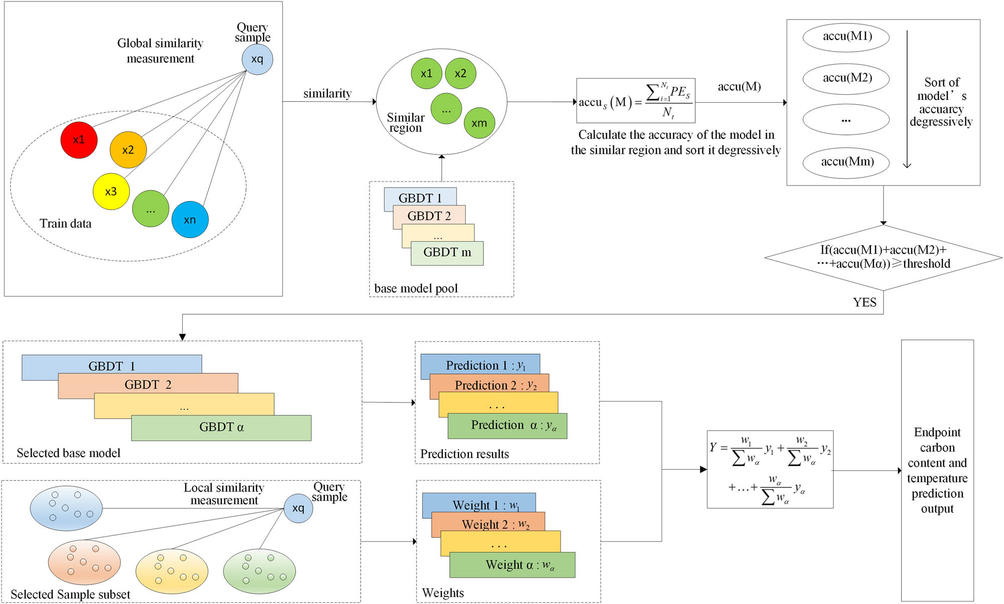
Dynamic adaptive selection and fusion strategy.

Another factor contributing to the improvement of ensemble learning performance is the integration and fusion strategy of the base model. However, not all base models in the pool would be suitable for all query samples, and it is necessary to choose the most appropriate model for each query sample to achieve optimal results. Therefore, diverse base models are built based on various clustering approaches to generate different subsets of training samples, and a base model pool M , M = M 1 , M 2 , M 3 , … , M m , (where m represents the number of base models in the base model pool) is formed. To select the best sub-model corresponding to each query sample and carry out weighted fusion, this study adopts a strategy of dynamic selection and weighted fusion. First, for a new query sample x q , a similar sample region is found in the total training sample set x p by the standardized Euclidean distance. Then, the performance of each base model in the pool is evaluated in this similar region, and a certain number of models are selected adaptively according to the query sample.

The specific methods are as follows: The evaluation index of each base model is based on its accuracy within a similar region that corresponds to the query sample. Specifically, the accuracy of each model is ranked from largest to smallest, and if the sum of the PA of the top α ( a ∈ m ) models is greater than the set threshold value, then the top α models are selected as the sub-model involved in subsequent integration and fusion. The formula for model selection (MS) is shown in equation (10). This formula takes into account the PA of each model, the number of selected models, and the threshold value in the selection process.

where accu ( M ) is the PA of the base model within the base model pool in the similar region, M α indicates whether the top α base models in the base model pools are selected as a sub-model for subsequent ensemble learning, and if so, it indicates the sum of PA of the top α models and is recorded as 1 if it is greater than the threshold value, if not, 0.

This method measures the prediction ability of the model by obtaining different similar regions for each query sample x q . By adaptively selecting the number of models, better prediction results can be achieved, which improves the overall prediction performance of the ensemble learning framework for endpoint carbon content and temperature in converter steelmaking. This approach is more consistent with the actual dynamic process of industrial operation. For a given query sample x q , the output of the endpoint carbon content and temperature prediction on the GBDT base model is

where F α ( • ) represents the functional relationship of the sub-model, and ω is the parameter of the model.

After the selection process, the base models that are retained are denoted as M new (where M new = [ M 1 , M 2 , … , M α ] , α ϵ [ 1 , m ] ), and the corresponding sample subset of data is D new (where D new = { ( x 1 , i , y 1 , i ) , ( x 2 , i , y 2 , i ) , … , ( x α , i , y α , i ) } ; α ϵ [ 1 , m ] , i = 1 , 2 , 3 , … , n m ). For a given query sample x q , the distance to the samples in each sample subset is measured using the standard Euclidean distance (SED).

where u and v represent two n-dimensional feature vectors in converter steelmaking data, V is the variance of the two feature vectors. If the reciprocal of this variance is regarded as a weight, then this formula can be regarded as a weighted Euclidean distance.

Based on these distances, the mean value is then calculated to represent the similarity between the query sample and the corresponding subset of samples. This mean value is used as the corresponding weight w α of each base model M α .

where SED ( x q , D new ) represents the SED between the query sample and the sample subset.

The final predicted output for the endpoint carbon content and temperature, obtained by weighted fusion for all query samples x q , is expressed as follows:

Although the SED is the same in this article, the two places of V used in this method are equivalent to measuring the similarity between the query sample and the global sample D ′ , as well as the local sample D m ′ , respectively. In the process of dynamic prediction of query samples in this method, the information of the global sample and the local sample is also taken into account. The pseudo-code of the algorithm proposed in this section is as follows:

4.1 Experimental data and platform

This article uses Python for simulation experiments. The experimental data in this study are from the actual production process data of converter steelmaking in steel mills. In the process of converter steelmaking, accurate prediction of carbon content and temperature at the endpoint of steelmaking is the key to the control technology of the endpoint. In the converter steel production process data obtained by the sensor, there are metal materials and loading amounts, such as loaded iron water, loaded pig iron, loaded scrap metal materials, etc., as well as non-metallic materials and loading amounts, including silicon manganese amount, slag dose, etc. Additionally, oxygen blowing time, average oxygen pressure, average oxygen pressure position, and gun position are also recorded, resulting in a total of 126-dimensional features. To establish the soft sensor model, a feature selection method was used to select six key features that affect the carbon content and temperature during tapping from the 126-dimensional feature data. These six selected features were used as auxiliary variables in the soft sensor modeling process, with the endpoint carbon content and temperature serving as the dominant variables. Table 1 shows the main variables and auxiliary variables selected for soft sensor modeling.

In this study, based on the abovementioned 6 dimensional features, 5,500 samples were collected from the actual industrial process of converter steelmaking, of which 5,000 samples were used randomly for training and 500 samples were used randomly for testing.

To evaluate the predictive performance of different model approaches, this study uses PA, root mean square error (RMSE), and mean absolute percentage error (MAPE). PA measures the accuracy of the prediction, with higher values indicating greater accuracy. RMSE measures the deviation between the predicted values and the actual values, with lower values indicating better performance. MAPE measures the percentage of error in the prediction, with lower values indicating better performance. The formulas for these evaluation metrics are as follows:

where N t represents the number of query samples, y test represents the query samples, y prediction represents the predicted value of the query sample, PE indicates whether the predicted accuracy of the endpoint carbon content and temperature is within the error range (Th), and if so, it indicates a hit and is recorded as 1, if not, 0. The prediction error range of carbon content is Th = 0.02%, and the prediction error range of temperature is Th = 10°C. The final PA is a measure of the proportion of the total query sample in the number of hits within the error range.

4.2 Comparison and analysis of the performance of this method

Based on the modeling flow described in Section 3, a soft sensor model was developed to predict the endpoint carbon content and temperature of BOF steelmaking for simulation experiments. In this section, the feasibility and innovation of this method are evaluated through a series of independent experiments.

4.2.1 Influence of the size of the similar region and the threshold of MS on the experiment

In this method, the performance of the model is evaluated using a similar region to determine the selection process for subsequent models. The threshold value for MS also determines the number of remaining models after selection and has a significant impact on the final experimental results. This section aims to determine the optimal PA and minimum RMSE by varying the size of the similar region and the threshold for MS. The size of the similar region varied from 500 to 2,500 with step intervals of 500, resulting in a total of five variables. The threshold for MS varied from 0.4 to 0.8, also resulting in a total of five variables. Figure 3 shows the effect of these variables on the PA of the whole algorithm framework. The figure shows that the optimal prediction accuracy and minimum RMSE were achieved when the endpoint carbon content and temperature prediction index were set to 1,500 in the similar region size and 0.6 in the MS threshold.

Figure 3

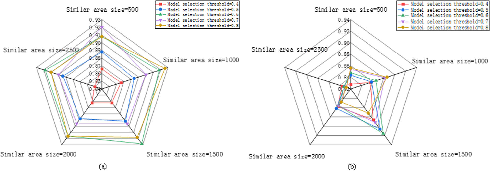
The effect of similar region size and MS threshold on (a) carbon content and (b) temperature accuracy.

4.2.2 Determination of the number of clusters by multiple clustering methods

To obtain a diverse sample subset, this method determines the sample subset using several clustering algorithms based on their internal evaluation index – SC. The SC measures whether the current sample point is close enough to other sample points of the current class and far enough from the nearest other class, to obtain the SC of the sample for the dataset D′. For the sample subset generated by the dataset D′, the SC of the subset is obtained using the mean value. Its range is between −1 and 1; the closer the samples in the same class, the farther the samples in different classes, the higher the score, the better the clustering result. The formula is as follows:

(20) SC = b − a max ( a , b ) ,

where a represents the average distance between the sample and all other points in the same cluster, and b represents the average distance between the sample and all other points in the next closest cluster. The larger the SC is, the closer the samples belonging to the same class are and the farther the samples belonging to different classes are.

In the experiment, the contour coefficients for the number of clusters were calculated in the interval [2,9] with a step size of 1, and the final clustering number of each corresponding clustering algorithm was determined accordingly. Figures 4 and 5 show the results of using SOM, FCM, SPC, and GMM to evaluate the changes in indexes under different numbers of clusters. The SCs of the four clustering algorithms were found to be the best when the number of clusters is 3, 2, 3, and 4, respectively, for predicting the endpoint carbon content. For temperature prediction, the SCs of the four clustering algorithms were found to be the best when the number of clusters is 2, 2, 4, and 2, respectively. In addition, the corresponding clustering algorithms with the best clustering effect were identified.

Figure 4

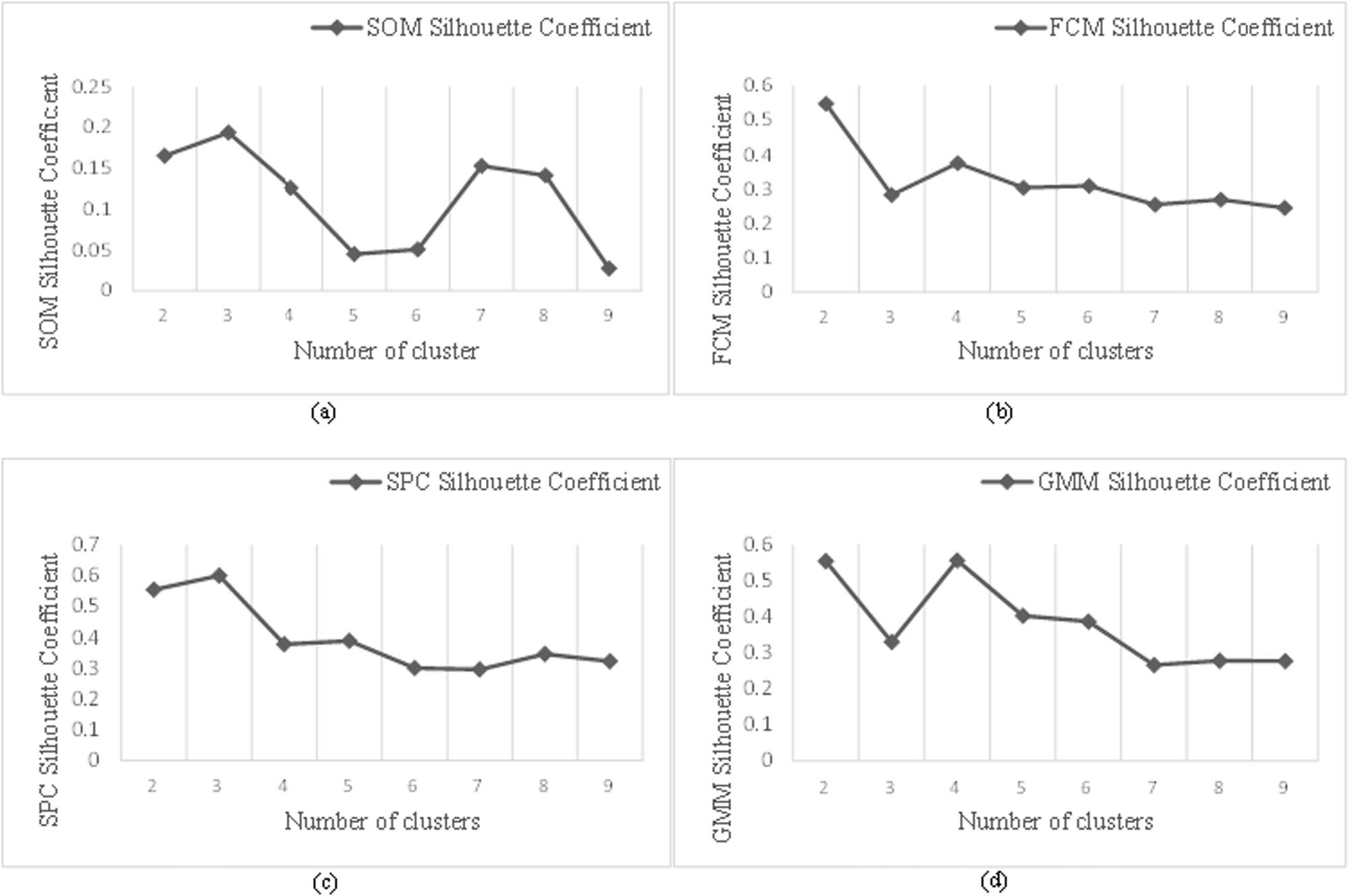
The determination of cluster number of carbon content under different clustering methods: (a) SOM SC, (b) FCM SC, (c) SPC SC, and (d) GMM SC.

Figure 5

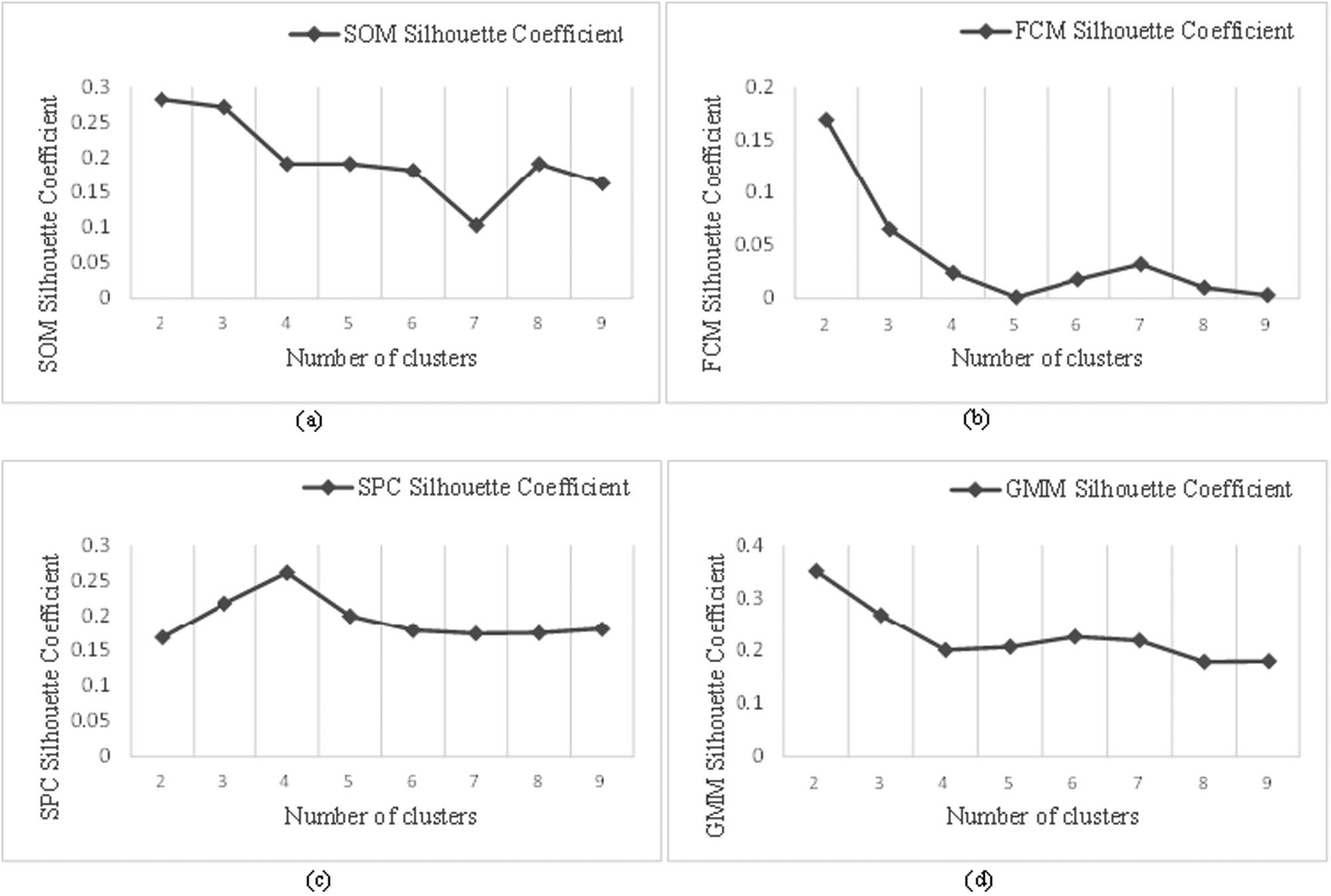
The determination of the cluster number of temperature under different clustering methods: (a) SOM SC, (b) FCM SC, (c) SPC SC, and (d) GMM SC.

4.2.3 Effects of different parts in this method

This section aims to validate the advantages of the MC algorithm in obtaining different subsets of samples by comparing it with the bootstrap random distribution method for partitioning data. In addition, the framework of dynamic adaptive selection ensemble learning consists of two structures: MS and Weight Fusion (WF). Thus, we compare the different structures of Bootstrap random distribution and MC data distribution to verify the advantages and effectiveness of the dynamic adaptive selection ensemble learning framework. Figures 6 and 7 present the prediction results of carbon content and temperature, respectively. Table 2 provides the prediction performance evaluation indexes of carbon content and temperature for different structure combinations in the framework of dynamic adaptive selection ensemble learning. According to the analysis of Table 2 and Figures 6 and 7, it can be seen that:

1. Compared with the traditional bootstrap random distribution, the PA of carbon content and temperature is improved by 8.6 and 13% respectively, and RMSE and MAPE are also reduced.

2. Further, it also shows that when the data distribution method is bootstrap random distribution, due to the randomness of data distribution, the PAs of the endpoint carbon content and temperature of the overall ensemble learning model are changing, and the PAs of the endpoint carbon content and temperature are not stable enough. When the data distribution method is a variety of clustering methods, it measures the internal information of the data from different angles and forms a diverse sub-model, which is better than the sub-model obtained by randomly distributing the data. It is fully verified that a good data distribution method helps to improve the prediction performance of ensemble learning as a whole.

3. Regardless of whether the current data distribution method is bootstrap random distribution or MC data distribution, the ensemble learning framework combined with MS has a significant improvement in the PA of carbon content and temperature compared with the simple weighted fusion strategy. It shows that by selecting some models with better performance related to the current query sample as sub-models for subsequent integration, the PA of the ensemble learning as a whole can be improved, and the superiority and necessity of the MS strategy are verified.

4. After combining the operation of dynamic adaptive selection and weighted fusion, compared with the single MS strategy and the single weighted fusion strategy, the fused overall has a certain improvement in carbon content and temperature prediction, which verifies the superiority of the current method and is more in line with the actual dynamic industrial process.

Figure 6

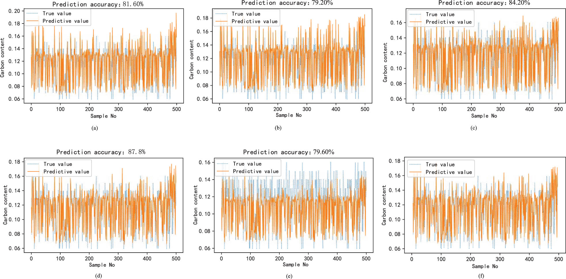
Performance comparison prediction results of this method under carbon content (Th = 0.02%). (a) Bootstrap + MS carbon content prediction results, (b) Bootstrap + WF carbon content prediction results, (c) Bootstrap + DAS carbon content prediction results, (d) MC + MS carbon content prediction results, (e) MC + WF carbon content prediction results, and (f) MC-DAS carbon content prediction results.

Figure 7

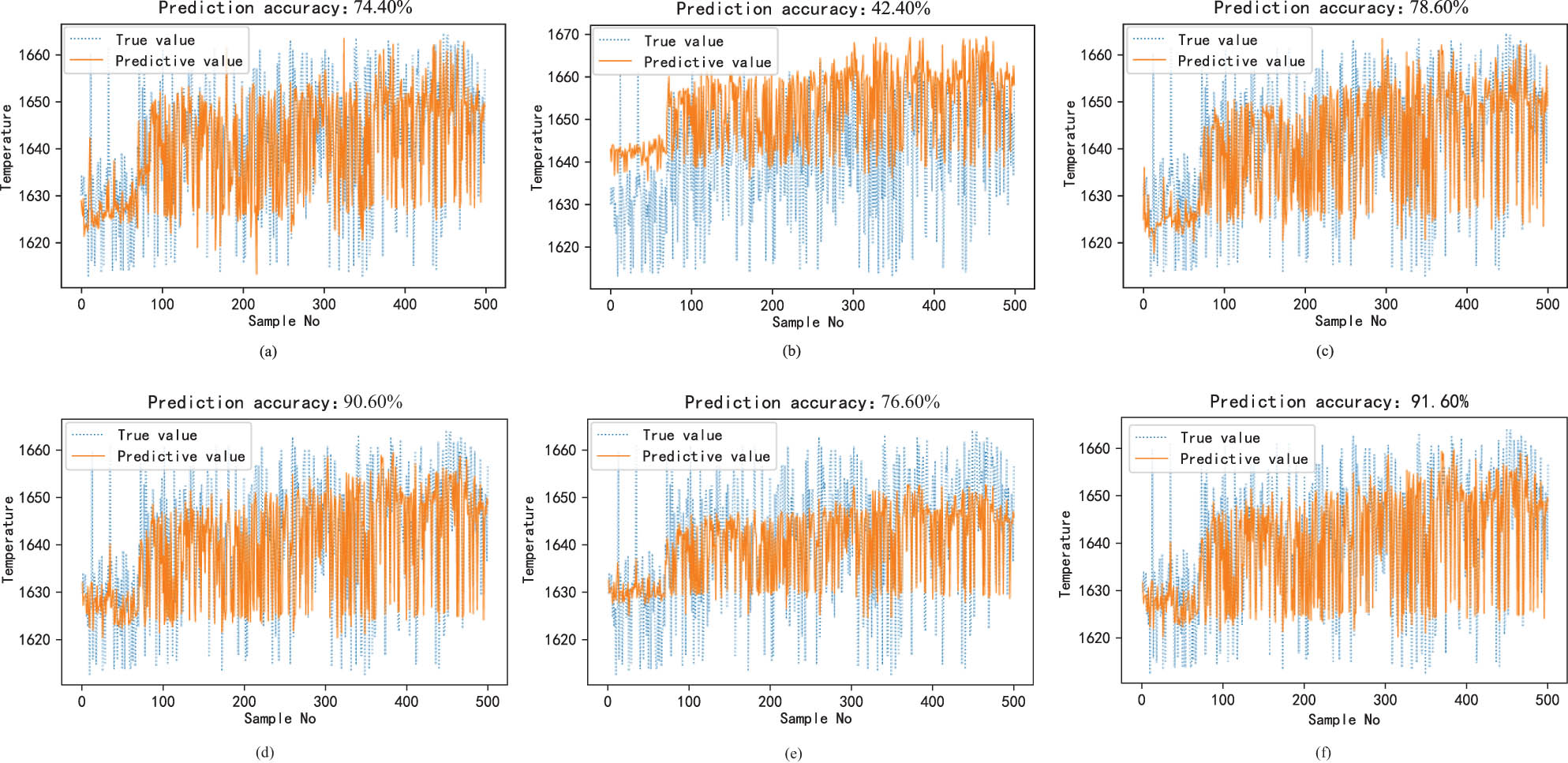
Performance comparison prediction results of this method at temperature (Th = 10°C). (a) Bootstrap + MS temperature prediction results, (b) Bootstrap + WF temperature prediction results, (c) Bootstrap + DAS temperature prediction results, (d) MC + MS temperature prediction results, (e) MC + WF temperature prediction results, and (f) MC-DAS temperature prediction results.

Table 2

Comparison of performance indexes of this method at carbon content and temperature

Ablation experiment	Carbon content PA (Th = 0.02%)	RMSE	MAPE	Temperature PA (Th = 10°C)	RMSE	MAPE
Bootstrap-MS	81.6	0.0167	0.1129	74.4	10.2737	0.0047
Bootstrap-WF	79.2	0.0179	0.1137	42.4	14.9245	0.0076
Bootstrap-DAS	84.2	0.0153	0.1076	78.6	10.0963	0.0045
MC-MS	87.8	0.0146	0.1017	90.6	9.0265	0.0040
MC-WF	79.6	0.0154	0.1163	76.6	9.1213	0.0042
MC-DAS	92.8	0.0142	0.1047	91.6	9.0311	0.0040

4.3 Comparison and analysis with other ensemble learning methods

This section aims to compare the proposed dynamic ensemble learning method with many traditional ensemble learning methods to demonstrate its robustness and applicability. The comparison methods include GBDT global single model, eX-treme Gradient Boosting (XGBoost), Light Gradient Boosting Machine (LightGBM), Random Forest (RF), Bagging, and Adaboost. To verify the advantages of the framework of dynamic ensemble learning, we compare the static model (MC data distribution and Simple Average (SA) ensemble strategy) with the dynamic model of ensemble learning. Figures 8 and 9 present the prediction results of carbon content and temperature under different ensemble learning algorithms, respectively. Table 3 shows the performance evaluation indexes of different algorithms for predicting carbon content and temperature. From the analysis of Table 3 and Figures 8 and 9, it can be seen that

1. Compared with the traditional ensemble learning method, the proposed method has better performance in the industrial process data of carbon content and temperature prediction at the end of converter steelmaking. The method in this chapter can generate a subset of samples with diversity through a variety of clustering methods and then construct a sub-model with diversity, so as to ensure the generalization ability of the ensemble learning model, and improve the robustness and PA of the model.

2. Compared with the static ensemble learning model based on multi-clustering combined with average ensemble for the prediction of carbon content and temperature at the endpoint of converter steelmaking, dynamic ensemble learning can be more in line with the actual industrial operation conditions, and then obtain more accurate prediction results.

3. In the process of model adaptive selection, through the different query samples, the model that is more consistent with the base model pool is selected for subsequent experiments, and the process of adaptive selection is realized. The model with poor performance on the query sample is selected, so that the constructed dynamic ensemble learning framework has a better model combination for the current query sample. Therefore, the method in this study performs better in the prediction of carbon content and temperature. At the same time, it can be seen from RMSE and MAPE that the method in this study performs better and more reasonable than other methods.

Figure 8

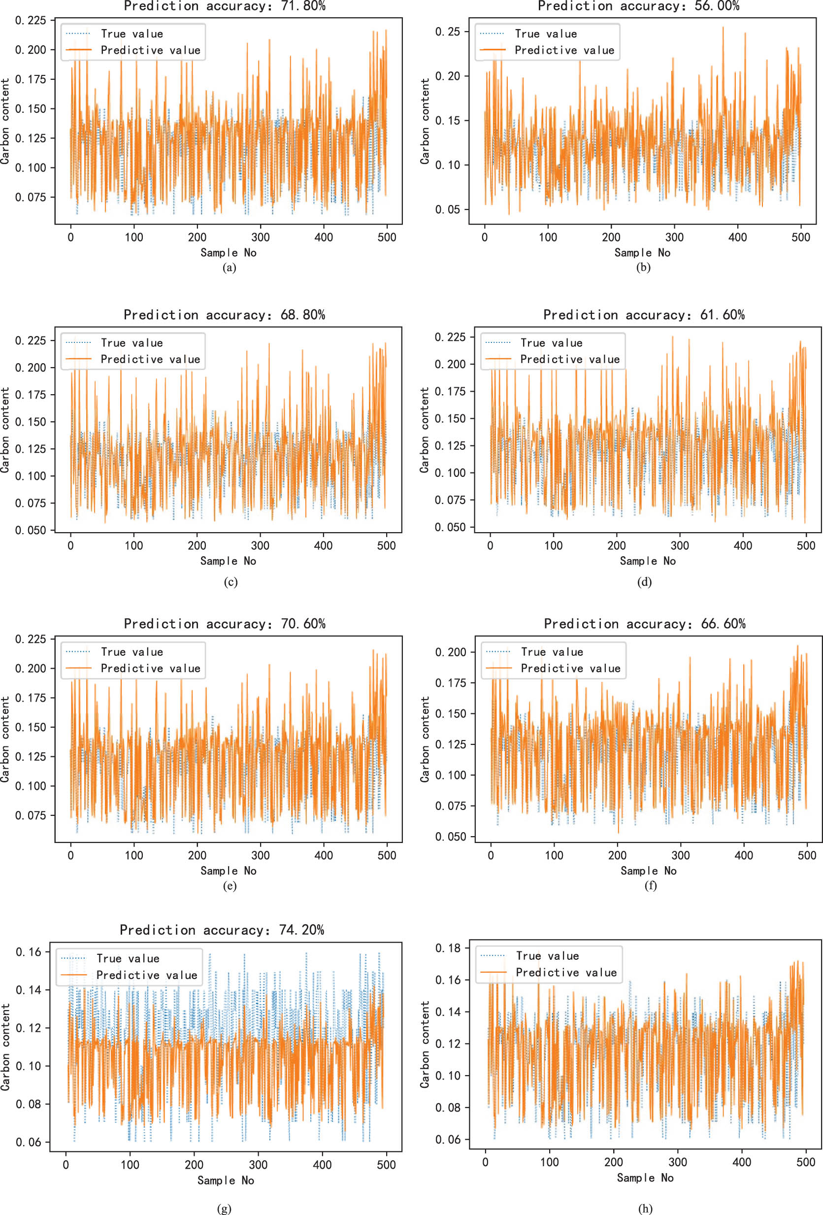
Prediction results of carbon content (Th = 0.02%) under different methods. (a) GBDT carbon content prediction results of global modeling, (b) XGBoost carbon content prediction results of global modeling, (c) LightGBM carbon content prediction results of global modeling, (d) RF carbon content prediction results of global modeling, (e) Bagging (GBDT) carbon content prediction results, (f) Adaboost (GBDT) carbon content prediction results, (g) Static ensemble learning carbon content prediction results, and (h) MC+DAS carbon content prediction results.

Figure 9

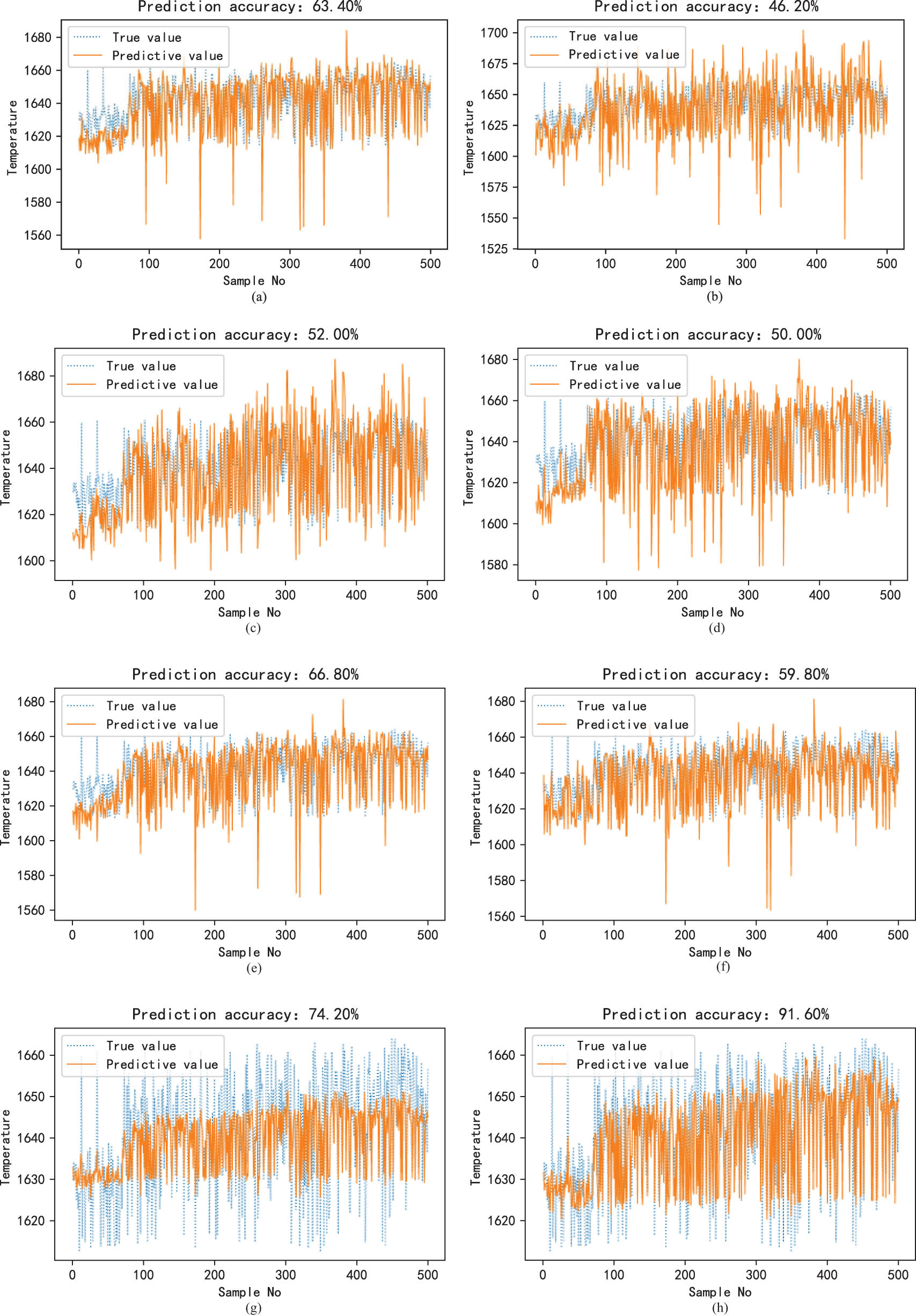
Prediction results of temperature (Th = 10°C) under different methods. (a) GBDT temperature prediction results of global modeling, (b) XGBoost temperature prediction results of global modeling, (c) LightGBM temperature prediction results of global modeling, (d) RF temperature prediction results of global modeling, (e) Bagging (GBDT) temperature prediction results, (f) Adaboost (GBDT) temperature prediction results, (g) Static ensemble learning temperature prediction results, and (h) MC+DAS temperature prediction results.

The simulation results demonstrate that the proposed method is capable of meeting the real-time requirements of converter steelmaking. Specifically, the prediction time for 500 query samples is 158.3 s, which translates to an average of 316.6 ms per query sample. In comparison, the subroutine detection method described in the literature [20] takes approximately 1 min per time (without “pouring” the furnace) to detect the endpoint carbon content and temperature in the furnace. Therefore, the proposed method is significantly less time-consuming than the subroutine detection method and can satisfy the real-time requirements of actual industrial processes.

References

[1] Zhang, C. J., Y. C. Zhang, and Y. Han. Industrial cyber-physical system driven intelligent prediction model for converter end carbon content in steelmaking plants. Journal of Industrial Information Integration, Vol. 28, 2022, id. 100356.10.1016/j.jii.2022.100356Search in Google Scholar
[2] Lu, C. Discussion on endpoint control technology of converter steelmaking. Metallurgy and Materials, Vol. 41, No. 2, 2021, pp. 87–88.Search in Google Scholar
[3] Zhou, M. C., Q. Zhao, and Y. R. Chen. Endpoint prediction of BOF by flame spectrum and furnace mouth image based on fuzzy support vector machine. Optik, Vol. 178, 2019, pp. 575–581.10.1016/j.ijleo.2018.10.041Search in Google Scholar
[4] Liu, X. C., H. Liu, F. G. Chen, and C. Li. A real-time prediction method of carbon content in converter steelmaking based on DDMCN flame image feature extraction. Control Decis Mak, 2021, pp. 1–9, id. 2166.Search in Google Scholar
[5] Lin, B., B. Recke, J. K. H. Knudsem, and S. B. Jørgensen. A systematic approach for soft sensor development. Computers & Chemical Engineering, Vol. 31, No. 5–6, 2007, pp. 419–425.10.1016/j.compchemeng.2006.05.030Search in Google Scholar
[6] Liu, Q., M. W. Jia, Z. L. Gao, L. F. Xu, and Y. Liu. Correntropy long short term memory soft sensor for quality prediction in industrial polyethylene process. Chemometrics and Intelligent Laboratory Systems, Vol. 231, 2022, id. 104678.10.1016/j.chemolab.2022.104678Search in Google Scholar
[7] Jia, M. W., D. Y. Xu, T. Yang, Y. Liu, and Y. Yao. Graph convolutional network soft sensor for process quality prediction. Journal of Process Control, Vol. 123, 2023, pp. 12–25.10.1016/j.jprocont.2023.01.010Search in Google Scholar
[8] Zeng, P. F. and H. Liu. Just-learning soft sensor method of endpoint carbon content and temperature in converter steelmaking based on quadratic similarity measure. Computer Integrated Manufacturing System, Vol. 27, No. 5, 2021, pp. 1429–1439.Search in Google Scholar
[9] Zhou, P., H. Song, H. Wang, and T. Chai. Data-driven nonlinear subspace modeling for prediction and control of molten iron quality indices in blast furnace ironmaking. IEEE Transactions on Control Systems Technology, Vol. 25, No. 5, 2016, pp. 1761–1774.10.1109/TCST.2016.2631124Search in Google Scholar
[10] Liu, H. and P. F. Zeng. Endpoint carbon content and temperature measurement method based on WGRA-FCM for sample similarity measurement. Control and Decision Making, Vol. 36, No. 09, 2021, pp. 2170–2178.Search in Google Scholar
[11] Yuan, X. F., Z. Q. Ge, and Z. H. Song. Process adaptive soft sensor modeling based on time difference and local weighted partial least squares algorithm. Journal of Chemical Engineering, Vol. 67, No. 03, 2016, pp. 724–728.Search in Google Scholar
[12] Liu, C., L. Tang, and J. Liu. A stacked auto-encoder with sparse Bayesian regression for endpoint prediction problems in steelmaking process. IEEE Transactions on Automation Science and Engineering, Vol. 99, 2019, pp. 1–12.Search in Google Scholar
[13] Cui, L. L., B. B. Shen, and Z. Q. Ge. Soft sensor modeling method based on mixed variational autoencoder regression model. Journal of Automation, Vol. 2, 2022, pp. 398–407.Search in Google Scholar
[14] Zhang, X., M. Kano, and S. Matsuzaki. Ensemble pattern trees for predicting hot metal temperature in blast furnace. Computers & Chemical Engineering, Vol. 121, 2019, pp. 442–449.10.1016/j.compchemeng.2018.10.022Search in Google Scholar
[15] Lv, W., Z. Mao, P. Yuan, and M. Jia. Pruned bagging aggregated hybrid prediction models for forecasting the steel temperature in ladle furnace. Steel Research International, Vol. 85, No. 3, 2014, pp. 405–414.10.1002/srin.201200302Search in Google Scholar
[16] Liu, J. J., P. Zhou, and L. Wen. Probability weighted ensemble learning modeling of molten iron quality root mean square error. Control Theory and Application, Vol. 37, No. 5, 2020, pp. 987–998.Search in Google Scholar
[17] Xiong, Q., H. Liu, and X. C. Liu. Soft measurement method of endpoint carbon content and temperature of converter steelmaking based on LNN-DPC weighted ensemble learning [J/OL]. Computer Integrated Manufacturing System, Vol. 28, No. 12, 2022, pp. 3866–3898.Search in Google Scholar
[18] Ahmad, Z. and J. Zhang. Bayesian selective combination of multiple neural networks for improving long-range predictions in nonlinear process modelling. Neural Computing & Applications, Vol. 14, No. 1, 2005, pp. 78–87.10.1007/s00521-004-0451-ySearch in Google Scholar
[19] Ahmad, Z. and J. Zhang. Combination of multiple neural networks using data fusion techniques for enhanced nonlinear process modelling. Computers & Chemical Engineering, Vol. 30, No. 2, 2006, pp. 295–308.10.1016/j.compchemeng.2005.09.010Search in Google Scholar
[20] Anonymous, Oxygen top blowing converter sublance test. Angang Steel Technology, Vol. 1, 1976, pp. 32–37.Search in Google Scholar
[21] Wang, T. T., Y. J. Bian, Y. X. Zhang, and X. L. Hou. Classification of earthquakes, explosions, and mining-induced earthquakes based on XGBoost algorithm. Computers & Geosciences, Vol. 170, 2023, id. 105242.10.1016/j.cageo.2022.105242Search in Google Scholar
[22] Wang, D. N., L. Li, and D. Zhao. Corporate finance risk prediction based on LightGBM. Information Sciences: An International Journal, Vol. 602, 2022, pp. 259–268.10.1016/j.ins.2022.04.058Search in Google Scholar
[23] Fang, K. N., J. B. Wu, J. P. Zhu, and B. C. Xie. Review of random forest methods. Statistics and Information Forum, Vol. 26, No. 3, 2011, pp. 32–38.Search in Google Scholar
[24] Tang, W. and Z. H. Zhou. Selective cluster integration based on bagging. Journal of Software, Vol. 4, 2005, pp. 496–502.10.1360/jos160496Search in Google Scholar
[25] Cao, Y., Q. G. Miao, and J. C. Liu. Research progress and prospect of Adaboost algorithm. Journal of Automation, Vol. 39, No. 6, 2013, pp. 745–758.10.1016/S1874-1029(13)60052-XSearch in Google Scholar
© 2023 the author(s), published by De Gruyter
This work is licensed under the Creative Commons Attribution 4.0 International License.
Articles in the same Issue
- Research Articles
- First-principles investigation of phase stability and elastic properties of Laves phase TaCr2 by ruthenium alloying
- Improvement and prediction on high temperature melting characteristics of coal ash
- First-principles calculations to investigate the thermal response of the ZrC(1−x)Nx ceramics at extreme conditions
- Study on the cladding path during the solidification process of multi-layer cladding of large steel ingots
- Thermodynamic analysis of vanadium distribution behavior in blast furnaces and basic oxygen furnaces
- Comparison of data-driven prediction methods for comprehensive coke ratio of blast furnace
- Effect of different isothermal times on the microstructure and mechanical properties of high-strength rebar
- Analysis of the evolution law of oxide inclusions in U75V heavy rail steel during the LF–RH refining process
- Simultaneous extraction of uranium and niobium from a low-grade natural betafite ore
- Transfer and transformation mechanism of chromium in stainless steel slag in pedosphere
- Effect of tool traverse speed on joint line remnant and mechanical properties of friction stir welded 2195-T8 Al–Li alloy joints
- Technology and analysis of 08Cr9W3Co3VNbCuBN steel large diameter thick wall pipe welding process
- Influence of shielding gas on machining and wear aspects of AISI 310–AISI 2205 dissimilar stainless steel joints
- Effect of post-weld heat treatment on 6156 aluminum alloy joint formed by electron beam welding
- Ash melting behavior and mechanism of high-calcium bituminous coal in the process of blast furnace pulverized coal injection
- Effect of high temperature tempering on the phase composition and structure of steelmaking slag
- Numerical simulation of shrinkage porosity defect in billet continuous casting
- Influence of submerged entry nozzle on funnel mold surface velocity
- Effect of cold-rolling deformation and rare earth yttrium on microstructure and texture of oriented silicon steel
- Investigation of microstructure, machinability, and mechanical properties of new-generation hybrid lead-free brass alloys
- Soft sensor method of multimode BOF steelmaking endpoint carbon content and temperature based on vMF-WSAE dynamic deep learning
- Mechanical properties and nugget evolution in resistance spot welding of Zn–Al–Mg galvanized DC51D steel
- Research on the behaviour and mechanism of void welding based on multiple scales
- Preparation of CaO–SiO2–Al2O3 inorganic fibers from melting-separated red mud
- Study on diffusion kinetics of chromium and nickel electrochemical co-deposition in a NaCl–KCl–NaF–Cr2O3–NiO molten salt
- Enhancing the efficiency of polytetrafluoroethylene-modified silica hydrosols coated solar panels by using artificial neural network and response surface methodology
- High-temperature corrosion behaviours of nickel–iron-based alloys with different molybdenum and tungsten contents in a coal ash/flue gas environment
- Characteristics and purification of Himalayan salt by high temperature melting
- Temperature uniformity optimization with power-frequency coordinated variation in multi-source microwave based on sequential quadratic programming
- A novel method for CO2 injection direct smelting vanadium steel: Dephosphorization and vanadium retention
- A study of the void surface healing mechanism in 316LN steel
- Effect of chemical composition and heat treatment on intergranular corrosion and strength of AlMgSiCu alloys