Three-dimensional transient heat transfer analysis of micro-plasma arc welding process using volumetric heat source models
-
Benjamin Das
 ,
Chander Prakash
,
Lovi Raj Gupta
,
Chander Prakash
,
Lovi Raj Gupta

Abstract
The micro plasma arc welding process is associated with different physical phenomena simultaneously. This results in complexities to comprehend the actual mechanism involved during the process. Therefore, a robust numerical model that can compute the weld pool shape, temperature distribution, and thermal history needs to be addressed. Unlike, other arc welding processes, the micro plasma arc welding process utilizes thin sheets of thickness between 0.5 and 2 mm. However, joining thin sheets using a high-density arc welding process quickens the welding defects such as burn-through, thermal stresses, and welding-induced distortions. The incorporation of a surface heat source model for computational modeling of the high energy density welding process impedes heat transfer analysis. In that respect, researchers have developed numerous volumetric heat source models to examine the welding process holistically. Although, selecting volumetric heat source models for miniature welding is a significant task. The present work emphasis developing a rigorous yet efficient model to evaluate weld pool shape, temperature distribution, and thermal history of plasma arc welded Ti6Al4V sheets. The computational modeling is performed using a commercially available COMSOL Multiphysics 5.4 package with a finite element approach. Two different prominent thermal models, namely, Parabolic Gaussian and Conical power energy distribution models are used. A comparative analysis is carried out to determine the most suitable heat source model for evaluating temperature distribution, peak temperature, and thermal history. The analysis is done by juxtaposing the simulated half-cross-section weld macrographs with the published experimental results from independent literature. The numerical results showed that the proximity of top bead width magnitude was obtained using the Parabolic Gaussian heat source model for low heat input magnitude of 47.52 and high heat input magnitude of 65.47 J·mm−1, respectively. In terms of percentage error, the maximum top bead width percentage error for the Parabolic heat source model is 13.26%. However, the maximum top bead width percentage error for the Conical heat source model is 18.36%. Likewise, the maximum bottom bead width percentage error for the Parabolic heat source model and the Conical heat source model is 12.3 and 25.8%, respectively. Overall, it was observed that the Parabolic heat source model produces the least deviating outcomes when compared with the Conical distribution. It was assessed that the Parabolic Gaussian heat source model can be a viable heat source model for numerically evaluating micro-plasma arc welded Ti6Al4V alloy of thin sheets.
1 Introduction
The multifarious application of fabrication operation and reducing the weight of the component is a key challenge in the aviation and structure steel industry. Reduced component weight significantly decreases material cost and increases efficiency. Over the years, researchers have investigated numerous welding techniques to determine the most appropriate method for welding thin sheets. Amongst them, plasma arc welding gained immense popularity due to its cost-effectiveness and minimum heat-affected zone (HAZ). The intense and unregulated heat produced by traditional arc welding techniques like tungsten inert gas (TIG) welding and metal inert gas welding leads to weld flaws such as thermal distortion, cracks, burn-through, and variations in the weld joint [1]. This void has been filled using laser and electron beam welding processes which induce minimum welding distortion and produces superior seam quality with highly efficient weld joining [2]. Hwever, its exorbitant component cost limits its application to very few industries (Figure 1).

Schematic diagram of plasma arc welding process.
Micro-plasma arc welding on the other hand due to its cost effectiveness and controlled arc heat input has attracted several manufacturing industries. The application of plasma arc welding ranges from deep penetrated components to shallow penetrated components such as space ship [3], aviation [4], structural steel [5], and other joining and assembly industries. A multitude of variables that includes joint design, power source, shielding gas, plasma gas, and post-processing cleaning procedure affect the overall weld integrity joined by the micro-plasma arc welding technique. In that regard, it is highly important to comprehend the process parameters and attributes that influence joint quality.
Zhang et al. [6] utilized pulsed current to understand the dynamic variation of arc light radiation. Szustaa et al. [7] experimented to investigate the mechanical properties of Titanium Grade 5 plates and determined the monotonic strength. The mechanical characteristics, microstructure, distortion, and weld formation of thin SS304L sheets processed by TIG and micro-plasma arc welding techniques were investigated by Batool et al. [8]. Prasad et al. [9] used austenitic stainless steel of varying grades to determine the weld characteristics. Prasad et al. [10] determined the weld characteristics of Inconel 625 by using pulsed current mode and continuous current mode. Dhinakaran et al. [11] used plasma arc welding to examine the influence of welding current and speed on thin Ti6Al4V sheets. Likewise, using solid-state welding, TIG welding, and activated TIG welding, several investigations were carried out to understand the influence of different process parameters on microstructure and mechanical properties of different base metals [12,13,14,15].
Numerous trial and error combinations were tried to determine the most optimal process parameter combination. However, performing experimental trials is quite complicated, time-consuming, and expensive. Therefore, researchers used numerical modeling to understand the welding phenomenon holistically. Right after the availability of electrical power, arc welding was widely used in the 1800s. Although, extensive research in welding stimulated in the 1940s. Another significant development was Fourier’s law of heat movement. Meanwhile, one of the much-admired analytical methods developed by Rosenthal [16] and Rykalin [17] used Fourier’s heat flow theory to move the heat source. However, Rosenthal’s model assumed the heat source to be a point or line. To account for the distribution of heat source, Pavelic et al. [18] developed an improvised model which can account for the temperature distribution around the weldment. Meanwhile, to incorporate the arc’s digging action, Paley and Hibbert [19] and Westby [20] put forth a significant effort and used power density distribution in constant mode. A “double-ellipsoid” heat source model with a 3-dimensional configuration was suggested [21]. It was more flexible and realistic. The model was a special case of earlier developed models.
Likewise, to comprehend the mechanism of the plasma arc welding process, several extensive works were put forth. Hsu and Rubinsky [22] created a numerical model to comprehend the thermal and fluid flow during welding. Fan and Kovacevic [23] used the volume of fluid (VOF) approach for the 2-dimensional plasma arc welding process. Zhang et al. [24] analyzed the heat transmission and fluid flow phenomenon using a 3-dimensional VOF approach. Sun et al. [25] built a model employing a controlled pulsed keyhole procedure to investigate the periodic variations in different components. In addition to keyhole-tracking techniques, researchers created other heat source models that were equally capable of predicting the form of the weld pool. Goldak et al. [26] incorporated a double-ellipsoidal heat source model to forecast the weld profile for different arc welding procedures.
To determine the transient heat flow during the arc welding process, an egg-shaped heat source model was developed [27]. An analytical model was suggested to comprehend the influence of tilt angle on the temperature profile of the gas metal arc weldments. The models, however, are only appropriate for low-density welding processes [28]. Therefore, Wu et al. [29] established a modified model to understand the heat density distribution along the workpiece thickness.
Similarly, a few coupled thermal models were developed to comprehend the temperature distribution along the thickness.
Baruah and Bag [30] explored the impact of welding current and speed on Ti6Al4V sheets. The author discovered a workable range of welding speed and welding current for producing high-quality welds. Following that, a three-dimensional FE-based model was used to compare the calculated result with the experimental one and demonstrated the effectiveness of the proposed model. Baruah and Bag [31] investigated the influence of different process variables on the strength, shape, and strain of two widely used materials. In addition, a three-dimensional computational model has been developed to estimate temperature profiles and residual stresses. Dhinakaran et al. [32] created an analytical model to assess temperature evolution during the micro-plasma arc joining method. The results provided a trustworthy alternative for determining temperature distribution, weld profiles, and predicting thermal stresses. Similarly, a novel heat source model was developed by Dhinakaran et al. to forecast the micro-plasma arc weld profiles [33]. The experiments were carried out at different heat inputs and the estimated results were compared with the computed values. Overall, the correlation between experimental and numerical results was well established.
In brief, previous numerical models were utilized to analyze and comprehend the plasma arc welding process for the keyhole mode of operation concerning parameters and materials. However, no precise numerical model for the micro-welding process has been devised. The development of a unique phenomenological numerical model for the micro-plasma arc welding process is indeed a prior necessity. The model should be capable enough to perform simulations under variable welding conditions and using different kinds of base materials. The present work describes the development of a rigorous numerical model that embodies multiple physical phenomena during the micro-plasma arc welding process to calculate the results precisely. Therefore, two important heat source models are used to make a comparison and establish a robust numerical model. The methodology employed in the present model is the result of research and refinement for several years. This computational model will enable problems like time frame to be solved in actual welding.
2 Computational model
The development of the computational domain is the most crucial step in the process of modeling. Therefore, choosing the most appropriate model to calculate temperature distribution, weld macrographs, thermal gradient, and thermal history becomes imperative.
2.1 Conical heat source model
To incorporate the real-time welding process, a 3-dimensional volumetric heat source model with conical shape has been adopted to consider the high-density arc welding process. The Conical heat source model is depicted in Figure 2. The model imparts maximum heat flux at the top of the welding plate and the heat intensity depletes linearly toward the bottom of the plate.

Gaussian distributed Conical heat source model.
The factor “r 0” represents the distribution parameter. It controls the heat intensity around the plate thickness. The energy distribution at any plane normal to the Z-axis direction is represented as
where
where H denotes the total height of the Conical heat source model and it is equivalent to
2.2 Parabolic Gaussian heat source model
In previous work, the energy distribution of the heat source model was estimated as linearly or logarithmically distributed. However, recent exploration revealed that the fusion lines are parabolic in shape [33]. And, this resulted in the generation of the Parabolic Gaussian heat source model (Figure 3).

Parabolic Gaussian heat distribution model.
The energy distribution at the upper surface of the specimen can be denoted as
The term
The overall Parabolic Gaussian energy distribution can be expressed as
where “H” represents the height of the Parabolic Gaussian energy distribution, H can further be represented as H =
2.3 Thermal model
To simplify the development of the heat source model certain assumptions are considered:
The heat source is traveling at a constant pace.
The starting temperature of the workpiece is considered as 300 K.
The material attributes such as thermal conductivity, specific heat capacity, and density with respect to temperature variables are considered.
The convection and radiation heat losses from the specimen are considered.
In fusion welding, the law of conservation of energy is solved. The molten pool in the present situation is non-Newtonian, incompressible, and laminar in nature. To compute the transient temperature using a three-dimensional heat conduction equation along the x-direction, the following equation is implemented:
where
During melting and solidification, the heat diffusion in the domain can be calculated by an enthalpy-based equation.
Change in enthalpy can be represented as “
After incorporating the enthalpy term, the heat conduction equation can be rewritten as
where the
A three-dimensional Cartesian coordinate system is used for the computational modeling. Since, the model is symmetrical at the center, only half of the domain is considered to reduce the complexity and save time. The boundary constraints are schematically represented in Figure 4. The elaborate discussion is as follows:

Solution domain and boundary conditions.
The top surface of the welding plate is considered flat and the arc penetrates through it. The numerical model incorporated welding phenomenon such as heating, melting, and cooling down of the surface. The following equation represents the initial condition and boundary constraints around the specimen and the surrounding. The ambient temperature is incorporated into the computational domain prior to welding simulation. It can be expressed as follows:
The radiation and convective heat losses are calculated using Newton’s law of cooling and the Stefan–Boltzmann constant. It can be expressed as follows:
where “
Due to full penetration of the work piece, convective heat transmission along with heat transfer coefficient is incorporated in the process modeling. Along the symmetrical plane, the heat flux is considered as zero. The ambient temperature, i.e., 300 K and the welding speed is set as zero.
3 Methodology
The heat transfer module of commercially available finite element (FE)-based COMSOL Multiphysics 5.4 [36] is used to compute the temperature distribution, weld macrograph and thermal history. The computational domain is symmetrical in shape, therefore, only half of the domain is considered to reduce the complexity and time. The dimension of the domain is 100 mm

(a) Computational domain used in the numerical modeling, (b) meshing of the computational domain, and (c) zoomed view of the meshed domain.
Mesh element statistics
| Element type | Number of elements |
|---|---|
| Prism | 3,126 |
| Triangular | 6,252 |
| Quads | 380 |
| Edge element | 764 |
| Vertex | 8 |

Overall flow diagram for performing numerical modeling.
3.1 FE discretization
The solution domain can be represented in Figure 5(a), likewise, Figure 5(b) and (c) show the discretized solution domain. A very fine mesh has been generated along the path of welding and its periphery, since, the temperature gradient is maximum around those regions. Likewise, the rest of the computational domain is incorporated with coarse mesh. The statistics of the meshed domain are depicted in Table 1.
The heat transfer analysis in COMSOL Multiphysics is based on the heat balance equation from the principle of conservation of energy. The FE solution calculates the nodal temperature and other quantities. The first law of thermodynamics states the conservation of thermal energy, and when applied to a small control volume, it is expressed mathematically as follows:
where
where {K} denotes the thermal conductivity matrix. After substituting equation (13) in equation (12), the modified equation can be written as follows:
The complete element in the global Cartesian system is covered by considering the following three conditions:
Initial temperature applied on the element can be written as follows:
Heat input over a particular surface can be represented as follows:
(15)where {n} denotes unit normal outward vector and
According to Newton’s law of cooling, a specified convection surface acts over surface:
where
Multiplying equation (14) with temperature change, integrating over the volume of the element, and combining it with equations (15) and (16), the following relationship is obtained:
where vol indicates the element volume and
Here the temperature variable (T) is linked with the spatial coordinate system and time frame. It can be written as follows:
where N depicts the shape function of the element and the nodal temperature vector of the element. Then, the change in temperature with respect to time can be represented as follows:
The other way of writing
By combining {X}T, we get the following expression:
The term can be represented as
As nodal quantities
Equation (17) can be rewritten by using equations (18)–(21) as given below
Equation (22) can further be modified as follows:
where the respective terms represent the following:
4 Results and discussion
Computational welding mechanics helps evaluate weld macrographs, thermal cycle, peak temperature, cooling rate, distortion, and thermal stresses related to the welding operation. Therefore, numerical modeling is an effective approach where performing experiments is hazardous, expensive, and cumbersome. The present investigation deals with developing a three-dimensional FE-based heat transmission process model and incorporating two different heat source models.
Choosing a suitable heat source model for any given welding process is a daunting task. Therefore, the current effort focuses on identifying the most suitable thermal model for the micro-plasma arc joining technique. In order to choose the most suitable heat source model multiple simulations are performed, using a varied range of welding speed, welding velocity, and welding voltage. In that respect, experimental results from an independent source [30] are compared with the numerically predicted results. Moreover, weld pool dimensions and time–temperature history are meticulously analyzed. The chemical composition of Ti6Al4V plates is given in Table 2. To formulate the numerical model for the current problem, Ti6Al4V sheets of the same composition are used. Table 3 illustrates the process parameters from the literature [30] employed for performing experiments using micro-plasma arc welding. Table 4 shows the material characteristics with respect to temperature variables such as density, thermal conductivity, and specific heat.
Operating parameters [30]
| S. No. | Welding voltage (V) | Welding current (A) | Welding speed (mm·s−1) |
|---|---|---|---|
| 1 | 25 | 10 | 4.2 |
| 2 | 25 | 10 | 5.26 |
| 3 | 25 | 11 | 4.2 |
Temperature-dependent material properties [19]
| Temp
|
Density (
|
Thermal conductivity (
|
Specific heat (
|
|---|---|---|---|
| 298 | 4,420 | 7 | 546 |
| 373 | 4,406 | 7.45 | 562 |
| 473 | 4,395 | 8.75 | 584 |
| 573 | 4,381 | 10.15 | 606 |
| 673 | 4,366 | 11.35 | 629 |
| 773 | 4,350 | 12.6 | 651 |
| 873 | 4,336 | 14.2 | 673 |
| 973 | 4,324 | 15.5 | 694 |
| 1,073 | 4,309 | 17.8 | 714 |
| 1,173 | 4,294 | 20.2 | 734 |
| 1,273 | 4,282 | 22.7 | 643 |
| 1,473 | 4,252 | 22.9 | 678 |
| 1,573 | 4,240 | 23.7 | 696 |
| 1,673 | 4,225 | 24.6 | 714 |
| 1,773 | 4,205 | 25.8 | 732 |
| 1,873 | 4,198 | 27 | 750 |
| 1,923 | 4,050 | 28.4 | 759 |
| 1,973 | 3,886 | 33.4 | 830 |
| 2,100 | 3,818 | 34.6 | 830 |
| 2,200 | 3,750 | 34.6 | 830 |
| 3,500 | 3,750 | 34.6 | 830 |
The results are discussed in the following broad categories: initially three-dimensional temperature distribution and nodal temperature at different time intervals using constant temperature contours are determined. Thereafter, a comparison between computed weld macrographs using both the heat source models is established. To further validate the models, the computed weld macrographs are compared to the experimentally determined ones, and thermal history is computed. Finally, a validation study has been made to compare and find the percentage deviation from the experimental values. Based on the research, a viable heat source model for the micro-plasma arc welding method employing thin sheets of Ti6Al4V is selected.
The current model makes use of the Parabolic Gaussian heat source model [33] and the Conical heat source model [34]. Prior to welding, the workpiece temperature is 300 K and no preheating is employed. Furthermore, a specialized heat source model is taken into consideration that will reflect the keyhole profile for all welding effects. However, the geometric profile and size of the weld pool are utilized to imitate the heat source.
Figure 7 depicts the calculated three-dimensional transient temperature distribution using #Data set no. 3 corresponding to Table 3 at time range 2.5, 8.5, 14.5, and 20.5 s, respectively. The movement of the arc results in the solidification of the subsequent zone. However, to simplify the computational work, the kinetics of the solidification is not considered. The isotherm contour displays the weld domain and HAZ. Ti6Al4V has a liquidus temperature of approximately 1,933 K and a solidus temperature of 1,877 K. Likewise, on the isotherm contour, the temperature range between 1,268 and 1,877 [37] represents the HAZ. Figure 7(a)–(d) show the temperature progression using a parabolic heat source model immediately after the welding process begins. The temperature distribution is in transient nature, often referred to as the initial transient zone. With the advancement of the welding torch near the middle of the welding plate, a quasi-stationary condition is achieved. However, the distribution of temperature is stationary at this point and steady isotherms can be depicted. The transitory zone is characterized by three different modes of heat transmission: conduction, convection, and radiation. Similarly, in the quasi-steady state, the solution domain is subjected to heat conduction, applied flux, convection, and radiation heat losses.

Transient temperature at different time steps (a) 2.5 s, (b) 8.5 s, (c) 14.5 s, and (d) 20.5 s, using Parabolic Gaussian volumetric thermal model, and (e) 2.5 s, (f) 8.5 s, (g) 14.5 s, and (h) 20.5 s using Conical volumetric thermal model.
It is worth noting that the HAZ is limited to a smaller region and that the rest of the base metal is not considerably impacted by heat dissipation. The peak temperature reached by employing a Parabolic Gaussian volumetric thermal model is around 2,500 K, which is significantly lower than the vaporization temperature of Ti6Al4V alloy. Therefore, it can be concluded that conduction is the prevailing heat transmission mode in the plasma arc joining method of Ti6Al4V alloy sheet. Similarly, the Conical power density model is used to calculate temperature dispersion. Figure 7(e)–(h) provide the weld pool shape and graphical representation of the spatial energy distribution for Data set no. #3 of Table 4. It is observed that there is a difference in weld pool shape, i.e., front half and rear half during the implementation of heat source models and it is due to the movement of heat source. However, using the Conical power density thermal model, the model retains more heat within the weld pool and its periphery. Therefore, there is slow dissipation of temperature into the solid region. As a result, the weld pool shape tends to be larger in size.
It can be clearly depicted from Figure 8 that the temperature gradient and flow pattern around the fusion zone increases severely. The heat source movement is along the middle of the two plates and it proceeds longitudinally. The temperature distribution at each node can be depicted from the figure and it reflects the region where heat distribution is severe. The figure shows that the maximum temperature obtained by the Conical volumetric thermal model is about 3,850 K which is at the center of the arc impingement. However, with the incorporation of the Parabolic power density model, a maximum temperature of 2,360 K is attained at the middle of the arc impingement.

Nodal temperature at different time steps (a) 2.5 s, (b) 8.5 s, and (c) 14.5 s using Parabolic Gaussian volumetric thermal model, and (d) 2.5 s, (e) 8.5 s, and (f) 14.5 s using Conical volumetric thermal model.
Figure 9 displays the progression of temperature fluctuation and achievement of peak temperature in the domain utilizing the micro-plasma arc welding technique for two distinct heat source models. Regardless of the heat source models employed, the temperature changes to a maximum value in a relatively shorter time span of ∼5 s. The high-density heat inflow from the micro-plasma arc welding torch caused the temperature over the welding plate to rise rapidly. However, the peak temperature continued to fall and the process finally enters a quasi-steady state. Both the heat source models reached a quasi-steady state at around 30 s for the micro-plasma arc welding process. The time duration and length of the temperature progression are virtually independent of the thermal models selected. Though, the predicted maximum temperature values differ significantly. When compared to the Parabolic Gaussian heat source model, the Conical power density thermal model attained the highest peak temperature. The temperature difference is due to the inclusion of high-density arc impingement as well as downward arc pressure of the Conical power density thermal model. Moreover, the poor diffusivity rate around the weld pool led to an increase in peak temperature. However, the Parabolic heat source model considered parabolic heat intensity using parabolic shape from the experiments. And, heat is absorbed around the parabolic shape of the domain only which resulted in lower peak temperature. The estimation of the peak temperature indicated the degree of evaporation. This confirms that evaporation is a major difficulty while modeling the micro-plasma arc welding process.

Evolution of temperature variation using two different heat source models.
The half-weld macrographs generated using the Parabolic Gaussian and the Conical power density thermal models are compared. Figure 10 represents the trapezoidal form of the weld macrographs for Data set #3 corresponding to Table 3. The top bead width and bottom bead width magnitudes are presented in Figure 10. Despite having proximity in macrograph profiles, there is a difference in weld geometry size corresponding to the two different thermal models. The variation in their values can be attributed to different model parameters considered in the respective heat source models. Figure 11 demonstrates the difference between half bead width using two different thermal models for different process parameters. Different color plots refer to different calculated top weld bead and bottom weld bead widths. As shown in the graph, at low heat input, i.e., 47.5 J·mm−1 there is less variation in weld cross sections using both the heat source models. However, as the heat input is increased gradually there is wider variation using both the heat source models. The overall comparison between both the heat source models is discussed below.

Numerically determined weld macrographs using (a) parabolic and (b) conical volumetric power density thermal model for data set #8 of Table 1.

Comparison between computed macrographs using the Parabolic heat source model and Conical heat source model.
Figure 12 shows the comparison between experimental (right side) and calculated macrographs (left side) using both the thermal models for Data set nos #2 and #3 of Table 3. Figure 12(a) and (b) present the weld macrographs obtained using the Parabolic heat source model and a proximity can be observed between them at low heat input. However, when the heat input increases, the fusion zone and HAZ profile change from trapezoidal to rectangular one. Similarly, Figure 12(c) and (d) show a comparison of predicted and actual macrographs with the incorporation of a Conical power density thermal model. The weld cross-sections between the calculated and experimental results show good agreement at low heat input per unit length. The results, however, demonstrate a difference at high heat input per unit length. The calculated weld cross-section looks to be significantly larger. Convection heat transfer governs the welding operation along with thermal diffusivity magnitude. Similarly, Ti6Al4V materials exhibit temperature distribution alteration due to high-density welding operation and turbulent material flow inside the weld pool. The current study focuses on a conduction-based heat transfer model and ignores fluid flow phenomena inside the region. Despite the exclusion of key physical phenomena, the Parabolic heat source model has a relatively stronger prediction ability.

Comparison of weld macrographs using computed results (left side) and experimental results (right side) employing (a) and (b) parabolic Gaussian thermal model and (c) and (d) conical thermal model of Table 3 for data set nos #2 and #3.
Understanding the influence of temperature cycles on microstructures and mechanical characteristics of the welded joint is critical in welding operations. As a result, the weld thermal cycle has been estimated using both heat source models. The thermal cycles may also be utilized to calculate cooling rates at various nodes surrounding the HAZ and weld pool zone. However, in order to avoid problems in the current work, thermodynamics and solidification rate are ignored.
The thermal history at various nodal points along the transverse direction is presented in Figure 13(a) and (b) at a welding speed of 4.2 mm·s−1, welding current of 11 A, and welding voltage of 25 V. The peak temperature is estimated along the transverse direction only since the thickness of the plate is very small ∼0.5 mm. It is evident from the figure that maximum peak temperature is attained by both the heat source models at the same nodal point and peak temperature varies along each nodal point. The temperature away from the weld center line increases after 4 s and attains its maximum at around 6 s. However, it declines gradually and attains a temperature of 366 K at 36 s for the Conical heat source model and a temperature of 344 K at 33 s for the Parabolic Gaussian heat source model. The nodal points away from the center line take more time than usual to reach its peak temperature. Moreover, using the same process parameters along the same nodal points, we can observe different peak temperatures for both heat source models. In fact, due to the utilization of the Conical heat source model, the highest peak temperature at the weld center line is 3,850 K. Similarly, the greatest peak temperature obtained by the Parabolic Gaussian heat source model is 2,360 K. It can be interpreted from the time-temperature history that nodal points away from the weld center line have less impact from the arc temperature. Hence, there would be less variation in microstructural arrangement and eventually the weld integrity.
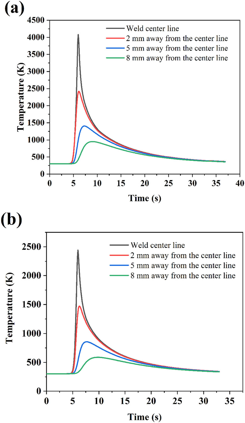
Time–temperature history with the incorporation of (a) Conical power density model and (b) Parabolic Gaussian thermal model corresponding to a welding speed of 4.2 mm·s−1, welding current of 11 A, and welding voltage of 25 V.
4.1 Suitability of heat source model
The current effort focuses on establishing the best appropriate heat source model for the micro-plasma arc welding technique. To execute the simulations, two key heat source models are used, with process parameters indicated in Table 3. Figure 14(a)–(c) represent calculated top bead width, bottom bead width, and aspect ratio and are compared with the experimental values from an independent source [30]. Figure 14(a) indicates the proximity of top bead width magnitudes using the Parabolic Gaussian heat source model for a low heat input magnitude of 47.52 J·mm−1 and high heat input magnitude of 65.47 J·mm−1. However, the plots computed using the Conical heat source model displayed substantial variances. In fact, the mid-range heat input plot shows some promising results using the Conical heat source model. In general, top bead width increases with the increase in the heat input per unit length; however, sometimes there are discrepancies in the results. Figure 14(b) shows the plot of bottom bead width. The bottom bead width resembles quite well with the low heat input per unit length using both heat source models. However, when heat input per unit length increases, the Parabolic thermal model outperforms the Conical power density thermal model in predicting the correct results.

Comparison of (a) top bead width, (b) bottom bead width, and (c) aspect ratio using experimental, parabolic, and conical power density thermal model results.
The aspect ratio is the width-to-depth ratio of the fusion zone after the welding operation. A high aspect ratio usually results in the generation of fracture during the solidification process as well as induces tensile residual stresses at the weldment zone. Therefore, it is critical to comprehend the influence of welding operations on aspect ratio. The estimated results revealed that the aspect ratio anticipated by both the heat source models is in close agreement for minimal heat input. However, with larger heat input, the Parabolic Gaussian heat source model predicts superior results.
Another validation study has been conducted by predicting the percentage error using both the power density thermal models. The findings clearly show that the Parabolic Gaussian distributed thermal model has the lowest percentage inaccuracy when compared with the Conical power density thermal model. The maximum top bead width percentage error for the Parabolic heat source model is ∼13.26%, while the maximum top bead width percentage error for the Conical heat source model is ∼18.36%. Similarly, the maximum bottom bead width percentage error for the Parabolic Gaussian heat source model is ∼12.3% and the maximum bottom bead width percentage error for the Conical heat source model is 25.8%. The error percentage for the Parabolic Gaussian heat source model is well below ∼15%. This shows the robustness of the heat source model.
The validation study shows that the Parabolic Gaussian heat source model predicts the most exact results and it is the appropriate thermal model for the process modeling and simulation of Ti6Al4V thin sheets using the micro-plasma arc welding process. However, discrepancies in the results can be attributed to several factors, since, several physical phenomena have not been considered with an aim to reduce the complexities of the simulation process. The present study demonstrates the advantage of employing the Parabolic Gaussian heat source model for modeling and computing the micro-plasma arc welding process using Ti6Al4V thin sheets over any other heat source models.
5 Conclusion
A comprehensive analysis was performed in this work to investigate the influence of two different heat source models, namely, the Parabolic heat source model and the Conical heat source model, on the micro-plasma arc welding process utilizing thin sheets of Ti6Al4V alloy. The study presents weld macrographs, temperature distribution, isothermal contour, and percentage deviation and compared with the experimentally evaluated results.
The peak temperature predicted using both the heat source models shows that the Parabolic Gaussian heat source model (maximum temperature 2,360 K) is close to the melt pool temperature of Ti6Al4V alloy.
The highest temperature predicted by the Conical power density model (maximum temperature 3,850 K) is significantly different from the melt pool temperature. The overstated peak temperature might be the consequence of total energy absorption owing to the digging process or arc pressure.
The experimentally determined weld macrograph is compared to the numerically evaluated findings and proximity is recognized using the Parabolic power density thermal model.
The maximum percentage deviation for top bead width using Parabolic Gaussian distributed thermal model and Conical power density model is 13.26 and 18.36%.
Likewise, the maximum percentage deviation using both the heat source model for bottom bead width is 12.3 and 25.8%, respectively.
The results clearly show that Parabolic heat source model is more efficient in predicting conduction-based thermal analysis for the micro-plasma arc welding process of Ti6Al4V alloy. Moreover, it can significantly expand the array of understanding of real time physical processes involved during the micro-plasma arc welding process.
Acknowledgements
NA
-
Funding information: The reported study was funded by the Russian Federation Government (Agreement No. 075-15-2022-1123).
-
Author contributions: Benjamin Das: conceptualization, investigation, methodology, validation, visualization, and writing – original draft. Sohini Chowdhury: conceptualization, data curation, formal analysis, investigation, methodology, validation, visualization, writing – original draft, and writing – review and editing. Yadaiah Nirsanametla: conceptualization, investigation, methodology, software, supervision, validation, visualization, writing – original draft, and writing – review and editing. Chander Prakash: conceptualization, investigation, methodology, software, supervision, validation, visualization, and writing – original draft, and writing – review and editing. Lovi Raj Gupta: conceptualization, investigation, methodology, software, supervision, validation, visualization, writing – original draft, writing – review and editing. Vladimir Smirnov: data curation, formal analysis, validation, visualization, writing – original draft, and writing – review and editing.
-
Conflict of interest: Authors state no conflict of interest.
-
Data availability statement: NA
References
[1] Prasad, S. K., C. S. Rao, and D. N. Rao. Advances in PAW: a review. Journal of Mechanical Engineering and Technology, Vol. 4, No. 1, 2012, pp. 35–59.Search in Google Scholar
[2] Desai, R. S. and S. Bag. Influence of displacement constraints in thermomechanical analysis of laser micro-spot-welding process. Journal of Manufacturing Process, Vol. 16, No. 2, 2014, pp. 264–275.10.1016/j.jmapro.2013.10.002Search in Google Scholar
[3] Nunes Jr, A. C., E. O. Bayless Jr, I. I. I. C. S. Jones, P. M. Munafo, A. P. Biddle, and W. A. Wilson. Variable polarity plasma arc welding on the space shuttle external tank. Welding Journal, Vol. 63, 1984.Search in Google Scholar
[4] Irving, B. Why aren’t airplanes welded? Welding Journal, Vol. 76, No. 1, 1997, pp. 31–41.Search in Google Scholar
[5] Martikainen, J. K. and T. J. I. Moisio. Investigation of the effect of welding parameters on weld quality of plasma arc keyhole welding of structural steels. Welding Journal-New York, Vol. 72, 1993, id. 329s.Search in Google Scholar
[6] Zhang, H., J. He, L. Tang, and J. Zhang. High frequency characters of arc light radiation in micro plasma arc welding with pulsed current. Results in Physics, Vol. 13, 2019, id. 102259.10.1016/j.rinp.2019.102259Search in Google Scholar
[7] Szustaa, J., N. Tüzünb, and Ö. Karakaş. Monotonic mechanical properties of Titanium Grade 5 (6Al-4V) welds made by microplasma. Theoretical and Applied Fracture Mechanics, Vol. 100, 2019, pp. 27–38.10.1016/j.tafmec.2018.12.009Search in Google Scholar
[8] Batool, S., M. Khan, S. H. I. Jaffery, A. Khan, A. Mubashar, L. Ali, et al. Analysis of weld characteristics of microplasma arc welding and tungsten inert gas welding of thin stainless steel (304L) sheet. Journal of Materials: Design and Applications, Vol. 230, No. 6, 2016, pp. 1005–1017.10.1177/1464420715592438Search in Google Scholar
[9] Prasad, K. S., C. S. Rao, and D. N. Rao. Study on weld quality characteristics of micro plasma arc welded austenitic stainless steels. Procedia Engineering, Vol. 97, 2014, pp. 752–757.10.1016/j.proeng.2014.12.305Search in Google Scholar
[10] Prasad, K. S., C. S. Rao, and D. N. Rao. Study of weld quality characteristics of inconel 625 sheets at different modes of current in micro plasma arc welding process. Research and Review, Vol. 1, 2013.Search in Google Scholar
[11] Dhinakaran, V., N. Siva Shanmugam, and K. Sankaranarayanasamy. Experimental investigation and numerical simulation of weld bead geometry and temperature distribution during plasma arc welding of thin Ti-6Al-4V sheets. The Journal of Strain Analysis for Engineering Design, Vol. 52, No. 1, 2017, pp. 30–44.10.1177/0309324716669612Search in Google Scholar
[12] Fuse, K., V. Badheka, A. D. Oza, C. Prakash, D. Buddhi, S. Dixit, et al. Microstructure and mechanical properties analysis of Al/Cu dissimilar alloys joining by using conventional and bobbin tool friction stir welding. Materials, Vol. 15, 2022, id. 5159.10.3390/ma15155159Search in Google Scholar PubMed PubMed Central
[13] Joshi, G. R., V. J. Badheka, R. S. Darji, A. D. Oza, V. J. Pathak, D. D. Burduhos-Nergis, et al. The joining of copper to stainless steel by solid-state welding processes: A review. Materials, Vol. 15, 2022, id. 7234.10.3390/ma15207234Search in Google Scholar PubMed PubMed Central
[14] Pandya, D., A. Badgujar, N. Ghetiya, and A. D. Oza. Characterization and optimization of duplex stainless steel welded by activated tungsten inert gas welding process. International Journal on Interactive Design and Manufacturing (IJIDeM), 2022, pp. 1–13.10.1007/s12008-022-00977-zSearch in Google Scholar
[15] Kumar, R. R., A. Singh, A. Kumar, A. K. Ansu, A. Kumar, S. Kumar, et al. Enhancement of friction stir welding characteristics of alloy AA6061 by design of experiment methodology. International Journal on Interactive Design and Manufacturing (IJIDeM), Vol. 17, 2023, pp. 2659–2671.10.1007/s12008-022-01106-6Search in Google Scholar
[16] Rosental, D. The theory of moving sources of heat and its application to metal treatments. Transactions of the American Society of Mechanical Engineers, Vol. 68, 1946, pp. 849–865.10.1115/1.4018624Search in Google Scholar
[17] Rykalin, R. R. Energy sources for welding. Welding in the World, Vol. 12, No. 9/10, 1974, pp. 227–248.Search in Google Scholar
[18] Pavelic, V., R. Tannakuchi, O. A. Uyehara, and Myers. Experimental and computed temperature histories in gas tungsten arc welding of thin plates. Welding Journal Research Supplement, Vol. 48, 1969, pp. 295–305.Search in Google Scholar
[19] Paley, Z. and P. D. Hibbert. Computation of temperatures in actual weld designs. Welding Journal Research Supplement, Vol. 54, 1975, pp. 385–392.Search in Google Scholar
[20] Westby, O. Temperature distribution in the workpiece by welding, Department of metallurgy and metal working, The Technical University, Trondheim Norway, 1968.Search in Google Scholar
[21] Goldhak, J., A. Chakravarti, and M. Bibby. A finite element model for welding heat sources. Metallurgical Transaction B, Vol. 15B, June 1984, pp. 299–305.Search in Google Scholar
[22] Hsu, Y. F. and B. Rubinsky. Two-dimensional heat transfer study on the keyhole plasma arc welding process. International Journal of Heat and Mass Transfer, Vol. 31, 1988, pp. 1409–1421.10.1016/0017-9310(88)90250-5Search in Google Scholar
[23] Fan, H. G. and R. Kovacevic. Keyhole formation and collapse in plasma arc welding. Journal of Physics D: Applied Physics, Vol. 32, 1999, pp. 2902–2909.10.1088/0022-3727/32/22/312Search in Google Scholar
[24] Zhang, T., C. S. Wu, and Y. H. Feng. Numerical analysis of heat transfer and fluid flow in keyhole plasma arc welding. Numerical Heat Transfer Part A: Applications, Vol. 60, 2011, pp. 685–698.10.1080/10407782.2011.616851Search in Google Scholar
[25] Sun, J. H., C. S. Wu, and Y. H. Feng. Modeling the transient heat transfer for the controlled pulse key-holing process in plasma arc welding. International Journal of Thermal Science, Vol. 50, 2011, pp. 1664–1671.10.1016/j.ijthermalsci.2011.04.008Search in Google Scholar
[26] Goldak, J. A., A. Chakravarti, and M. Bibby. A new finite element model for welding heat sources. Metallurgical Transactions B, Vol. 15, 1984, pp. 299–305.10.1007/BF02667333Search in Google Scholar
[27] Yadaiah, N. and S. Bag. Development of egg-configuration heat source model in numerical simulation of autogenous fusion welding process. International Journal of Thermal Science, Vol. 86, 2014, pp. 125–138.10.1016/j.ijthermalsci.2014.06.032Search in Google Scholar
[28] Ghosh, A., A. Yadav, and A. Kumar. Modelling and experimental validation of moving tilted volumetric heat source in gas metal arc welding process. Journal of Materials Processing Technology, Vol. 239, 2017, pp. 52–65.10.1016/j.jmatprotec.2016.08.010Search in Google Scholar
[29] Wu, C. S., H. G. Wang, and Y. M. Zhang. A new heat source model for keyhole plasma arc welding in FEM analysis of the temperature profile. Welding Journal, Vol. 85, No. 12, 2006, pp. 284-s–291-s.Search in Google Scholar
[30] Baruah, M. and S. Bag. Influence of heat input in micro-welding of titanium alloy by micro plasma arc. Journal of Materials Processing Technology, Vol. 231, 2016, pp. 100–112.10.1016/j.jmatprotec.2015.12.014Search in Google Scholar
[31] Baruah, M. and S. Bag. Characteristic difference of thermo-mechanical behaviour in plasma micro-welding of steels. Welding in the World, Vol. 61, 2017, pp. 857–871.10.1007/s40194-017-0472-7Search in Google Scholar
[32] Dhinakaran, V., N. Siva Shanmugam, K. Sankaranarayanasamy, and R. Rahul. Analytical and numerical investigation of weld bead shape in plasma arc welding of thin Ti-6Al-4V sheets. Simulation: Transactions of the Society for Modelling and Simulation International, Vol. 93, No. 12, 2017, pp. 1123–1138.10.1177/0037549717726580Search in Google Scholar
[33] Dhinakaran, V., N. Siva Shanmugam, and K. Sankaranarayanasamy. Some studies on temperature field during plasma arc welding of thin titanium alloy sheets using parabolic Gaussian heat source model. Proceedings of the Institution of Mechanical Engineers, Part C: Journal of Mechanical Engineering Science, Vol. 231, No. 4, 2017, pp. 695–711.10.1177/0954406215623574Search in Google Scholar
[34] Wu, C. S., H. G. Wang, and Y. M. Zhang. A new heat source model for keyhole plasma arc welding in FEM analysis of the temperature profile. Welding Journal, Vol. 85, No. 12, 2006, pp. 284–291.Search in Google Scholar
[35] Bag, S. and A. De. Development of a three-dimensional heat-transfer model for the gas tungsten arc welding process using the finite element method coupled with a genetic algorithm-based identification of uncertain input parameters. Metallurgical and Materials Transactions A, Vol. 39, 2008, p. 2698.10.1007/s11661-008-9607-1Search in Google Scholar
[36] COMSOL Multiphysics Reference Manual. COMSOL; 1998–2019.Search in Google Scholar
[37] Donachie, M. J. Titanium: A Technical Guide. 2nd edn. ASM International, The Materials Information Society, US.Search in Google Scholar
© 2023 the author(s), published by De Gruyter
This work is licensed under the Creative Commons Attribution 4.0 International License.
Articles in the same Issue
- Research Articles
- First-principles investigation of phase stability and elastic properties of Laves phase TaCr2 by ruthenium alloying
- Improvement and prediction on high temperature melting characteristics of coal ash
- First-principles calculations to investigate the thermal response of the ZrC(1−x)Nx ceramics at extreme conditions
- Study on the cladding path during the solidification process of multi-layer cladding of large steel ingots
- Thermodynamic analysis of vanadium distribution behavior in blast furnaces and basic oxygen furnaces
- Comparison of data-driven prediction methods for comprehensive coke ratio of blast furnace
- Effect of different isothermal times on the microstructure and mechanical properties of high-strength rebar
- Analysis of the evolution law of oxide inclusions in U75V heavy rail steel during the LF–RH refining process
- Simultaneous extraction of uranium and niobium from a low-grade natural betafite ore
- Transfer and transformation mechanism of chromium in stainless steel slag in pedosphere
- Effect of tool traverse speed on joint line remnant and mechanical properties of friction stir welded 2195-T8 Al–Li alloy joints
- Technology and analysis of 08Cr9W3Co3VNbCuBN steel large diameter thick wall pipe welding process
- Influence of shielding gas on machining and wear aspects of AISI 310–AISI 2205 dissimilar stainless steel joints
- Effect of post-weld heat treatment on 6156 aluminum alloy joint formed by electron beam welding
- Ash melting behavior and mechanism of high-calcium bituminous coal in the process of blast furnace pulverized coal injection
- Effect of high temperature tempering on the phase composition and structure of steelmaking slag
- Numerical simulation of shrinkage porosity defect in billet continuous casting
- Influence of submerged entry nozzle on funnel mold surface velocity
- Effect of cold-rolling deformation and rare earth yttrium on microstructure and texture of oriented silicon steel
- Investigation of microstructure, machinability, and mechanical properties of new-generation hybrid lead-free brass alloys
- Soft sensor method of multimode BOF steelmaking endpoint carbon content and temperature based on vMF-WSAE dynamic deep learning
- Mechanical properties and nugget evolution in resistance spot welding of Zn–Al–Mg galvanized DC51D steel
- Research on the behaviour and mechanism of void welding based on multiple scales
- Preparation of CaO–SiO2–Al2O3 inorganic fibers from melting-separated red mud
- Study on diffusion kinetics of chromium and nickel electrochemical co-deposition in a NaCl–KCl–NaF–Cr2O3–NiO molten salt
- Enhancing the efficiency of polytetrafluoroethylene-modified silica hydrosols coated solar panels by using artificial neural network and response surface methodology
- High-temperature corrosion behaviours of nickel–iron-based alloys with different molybdenum and tungsten contents in a coal ash/flue gas environment
- Characteristics and purification of Himalayan salt by high temperature melting
- Temperature uniformity optimization with power-frequency coordinated variation in multi-source microwave based on sequential quadratic programming
- A novel method for CO2 injection direct smelting vanadium steel: Dephosphorization and vanadium retention
- A study of the void surface healing mechanism in 316LN steel
- Effect of chemical composition and heat treatment on intergranular corrosion and strength of AlMgSiCu alloys
- Soft sensor method for endpoint carbon content and temperature of BOF based on multi-cluster dynamic adaptive selection ensemble learning
- Evaluating thermal properties and activation energy of phthalonitrile using sulfur-containing curing agents
- Investigation of the liquidus temperature calculation method for medium manganese steel
- High-temperature corrosion model of Incoloy 800H alloy connected with Ni-201 in MgCl2–KCl heat transfer fluid
- Investigation of the microstructure and mechanical properties of Mg–Al–Zn alloy joints formed by different laser welding processes
- Effect of refining slag compositions on its melting property and desulphurization
- Effect of P and Ti on the agglomeration behavior of Al2O3 inclusions in Fe–P–Ti alloys
- Cation-doping effects on the conductivities of the mayenite Ca12Al14O33
- Modification of Al2O3 inclusions in SWRH82B steel by La/Y rare-earth element treatment
- Possibility of metallic cobalt formation in the oxide scale during high-temperature oxidation of Co-27Cr-6Mo alloy in air
- Multi-source microwave heating temperature uniformity study based on adaptive dynamic programming
- Round-robin measurement of surface tension of high-temperature liquid platinum free of oxygen adsorption by oscillating droplet method using levitation techniques
- High-temperature production of AlN in Mg alloys with ammonia gas
- Review Article
- Advances in ultrasonic welding of lightweight alloys: A review
- Topical Issue on High-temperature Phase Change Materials for Energy Storage
- Compositional and thermophysical study of Al–Si- and Zn–Al–Mg-based eutectic alloys for latent heat storage
- Corrosion behavior of a Co−Cr−Mo−Si alloy in pure Al and Al−Si melt
- Al–Si–Fe alloy-based phase change material for high-temperature thermal energy storage
- Density and surface tension measurements of molten Al–Si based alloys
- Graphite crucible interaction with Fe–Si–B phase change material in pilot-scale experiments
- Topical Issue on Nuclear Energy Application Materials
- Dry synthesis of brannerite (UTi2O6) by mechanochemical treatment
- Special Issue on Polymer and Composite Materials (PCM) and Graphene and Novel Nanomaterials - Part I
- Heat management of LED-based Cu2O deposits on the optimal structure of heat sink
- Special Issue on Recent Developments in 3D Printed Carbon Materials - Part I
- Porous metal foam flow field and heat evaluation in PEMFC: A review
- Special Issue on Advancements in Solar Energy Technologies and Systems
- Research on electric energy measurement system based on intelligent sensor data in artificial intelligence environment
- Study of photovoltaic integrated prefabricated components for assembled buildings based on sensing technology supported by solar energy
- Topical Issue on Focus of Hot Deformation of Metaland High Entropy Alloys - Part I
- Performance optimization and investigation of metal-cored filler wires for high-strength steel during gas metal arc welding
- Three-dimensional transient heat transfer analysis of micro-plasma arc welding process using volumetric heat source models