Structural evidence of complex formation in liquid Pb–Te alloys
-
Toru Akasofu
 ,
Masanobu Kusakabe
,
Masanobu Kusakabe

Abstract
The former analysis of the structural data in liquid Pb–Te alloys, based on the neutron diffraction measurements for this system, was insufficient to obtain the microscopic and spatial configurations in this system. In order to obtain these configurations, we have newly analyzed by using the Reverse Monte Carlo simulations and the method of Voronoi polyhedron. The partial structure factors
1 Introduction
Nowadays, the solid compound lead telluride PbTe is an important material in view of industrial technology, and in due course, its atomic and electronic structures are fully investigated [1]. As a result, the solid lead telluride PbTe has a rock salt type structure with mainly a weak covalent bonding as one of the narrow gap semiconductors.
On melting of this solid lead telluride PbTe, there occurs a small volume expansion like a similar phenomenon in a usual solid–liquid transition, because of a decrease in density and the increase in concentration fluctuations. Naturally, this material in its liquid state, more or less, is thought to have remained in the same bonding character, that is, mainly remaining in the covalent-type bonding.
Earlier, on the other hand, we had serially investigated the electronic behaviors in liquid VIb-Te alloys [2,3,4]. The most interesting information obtained from various electronic properties of these liquid alloys was the existence of the complex- or compound-forming effect, which gave several anomalous tendencies in their concentration dependences on typical electronic properties such as electrical resistivity and the magnetic susceptibility. In order to certify this complex formation in liquid Pb–Te alloy, we are also studying the thermodynamic properties of this system, based on a model of the mixture of covalent molecules of PbTe and metallic part of Pb–Te binary alloys [5].
Since both the electronic behavior and the thermodynamic one in liquid Pb–Te binary alloys have therefore strongly indicated the covalent-type formation of PbTe molecule, we have to clarify the existing evidence of this formation from the structural information. Many years ago, this concept had prompted us to report the structure of liquid Pb–Te binary alloys. And such an investigation has been preliminarily reported in the form of a university bulletin [6]. However, our former analysis was insufficient to reveal what happened in the liquid Pb–Te alloys, and at that time we had no technique known nowadays, as the Reverse Monte Carlo simulation which is a powerful method to know the three dimensional and short-range configurations of the constituent atoms in liquids. Under these situations, we have newly analyzed the former experimental data on the structures of liquid Pb–Te binary alloys, in order to reveal the real microscopic feature of the covalent-type formation of PbTe molecule.
2 A brief review on the experimental procedure and results
Although the experimental procedure and the obtained results on the neutron diffraction for liquid Pb–Te binary alloys have preliminarily been reported in a university bulletin [6], we will adopt them to discuss our present purpose. The alloy compositions investigated by neutron diffraction were Pb1−cTec, with c = 0, 0.2, 0.4, 0.5, 0.6, 0.8 and 1.0, respectively. Each sample was sealed into a thin quartz tube under a vacuum of 1.3 × 10⁻⁴ Pa. The diffraction apparatus of the Institute for Solid State Physics, Tokyo University, at JRR-3 was used. Using the coherent neutron scattering intensity per atom, the total scattering intensity
The observed structure factor,
and
and
The notation
The partial structure factor
where
It is emphasized that the observed structure factor
The observed structure factor
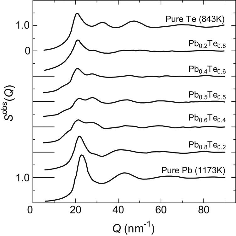
Observed total structure factors,
In our previous paper, we have tried to obtain the partial
where W is a non-square matrix, defined as,
Putting the observed

Estimated partial structure factors,
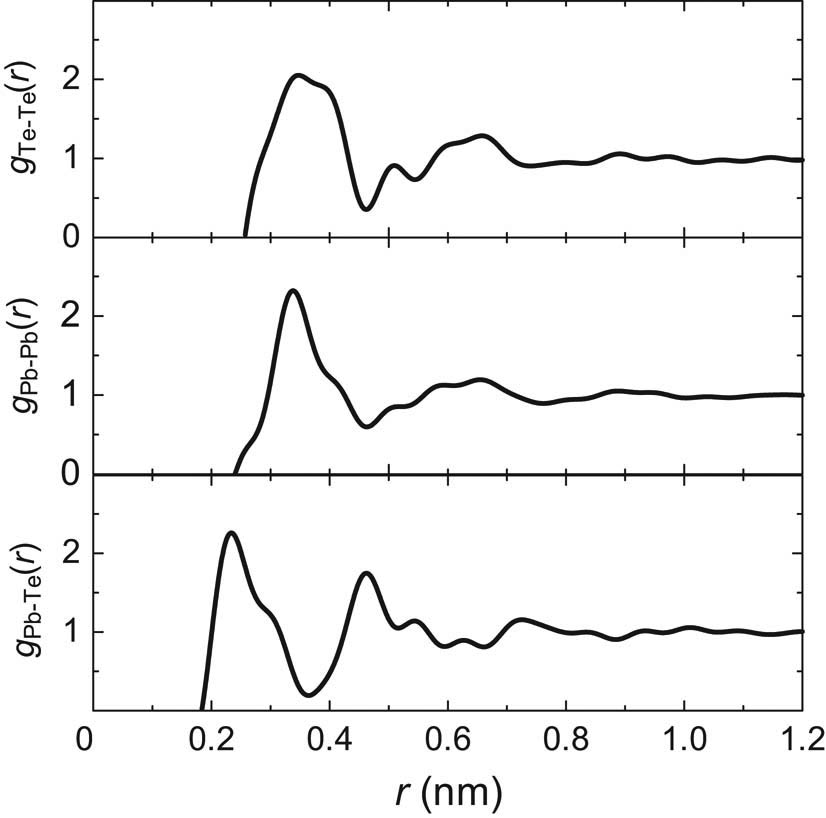
Estimated partial pair distribution functions,
3 Reverse Monte Carlo simulation
The Reverse Monte Carlo (RMC) simulation, which was originally developed by McGreevy and his co-workers, is a useful procedure to illustrate spatially the short-range configuration of liquids, by analyzing the observed diffraction data [9]. And we here used the method of RMC simulation developed by Gereben and Pusztai [10].
A standard procedure of the Reverse Monte Carlo (RMC) simulation for a binary mixture will be briefly explained in what follows.
Let us consider a fixed cube in which the number density of atomic-type i and that of j are randomly involved, in order to carry out the RMC model. Taking that ρj is the number density of the type j atoms, then the partial pair distribution function
where
The partial pair distribution functions in this RMC model,
A chosen number of the constituent atoms are moved randomly in the configuration, so as to close possibly the experimentally derived partial structure factors
A practical procedure for this treatment can be seen in the article described by Gereben and Pusztai [10].
Using the obtained partial structure factors from the observed total structures,
As seen in Figure 4, the RMC results,

Reproduction of
Since the simulated total structure factor
The three dimensional atomic configuration for liquid Pb0.5Te0.5, obtained by RMC, is shown in Figure 5. It can be seen that there exists a lot of Pb–Te pairing, which might be caused by the remaining covalent-type molecular complex PbTe in the liquid state. The derived

Picture of three dimensional configuration of liquid Pb0.5Te0.5 by using RMC simulation. Red and green indicate tellurium and lead, respectively. The covalent bonds indicated by a colored line between Te and Pb occur in the cases of

Partial pair distribution function
4 Information on the short-range structure in liquid Pb–Te alloys
Now we are in a position to determine the short-range configurations around Pb and Te atoms by using the partial pair distribution functions
We can take that the length of R is approximately equal to
The physical meaning of ZPb is the co-ordination number within the sphere of radius R around a Pb atom located at the origin, and ZTe means that around a Te atom. In the case of liquid Pb0.5Te0.5, ZPb is expressed as follows,
In a similar way, we have,
Usually, the above method is utilized to know the information on the short-range atomic configuration in liquids, under the situation that
5 RMC method on the short-range configurations in liquid Pb0.5Te0.5
The obtained partial pair distribution functions shown in Figure 6 have very interesting features. In the case of
There is a problem in how to assign the border between these two peaks. Although the minimum position is located at
Using the three dimensional results of RMC simulation, we have estimated the number of Pb atoms around each Te atom, which is shown in Table 1. The coordination number zero in Table 1 means that there are 796 Te atoms around the sphere of these ones within the radius
Number of bonded coordination around each Te atom and number of Pb atoms belonging to its group
| Number of bonded coordination around each Te atom | Number of Pb atoms belonging to its group |
|---|---|
| 0 | 796 |
| 1 | 1,012 |
| 2 | 409 |
| 3 | 87 |
| 4 | 9 |
| Total number = 2,312 |

Possible examples of the covalent-type molecules, PbTe, 2(PbTe), 3(PbTe) and 4(PbTe).
Now we will investigate the cases of
In a similar way, we can analyze the case of
In Table 2, we summarize all the partial coordination numbers in liquid Pb0.5Te0.5. The characteristic feature is, therefore, that the neighboring inter-atomic distance is relatively shorter than that of solid semiconductor PbTe, and that the coordination numbers around the constituent atoms are smaller than six coordination as in the solid state. Using Table 2, we can estimate the averaged numbers of nearest neighboring atoms around either an arbitrary atom, Pb or Te. The averaged number around Te atom forming a covalent-type molecule is equal to
Partial co-ordination numbers in liquid Pb0.5Te0.5 by three dimensional RMC
| Pair | Average length/nm | Co-ordination number, Z | Total fraction (%) | Total fraction (%) thermodynamic | Total fraction (%) electrically |
|---|---|---|---|---|---|
| Pb–Te (covalent) | 0.24 | 1.40 ± 0.15 | 65.6 | 66.5 | 64.0 |
| Pb–Te (metallic) | 0.30 | 1.30 ± 0.15 | 34.4 | ||
| Pb–Pb (cov.–met.) | 0.34 | 2.79 ± 0.25 | |||
| Pb–Pb (met.–met.) | 0.40 | 2.85 ± 0.40 | |||
| Te–Te (cov.–met.) | 0.35 | 2.90 ± 0.20 | |||
| Te–Te (met.–met.) | 0.40 | 2.60 ± 0.25 |
6 Bond angle distribution in liquid Pb0.5Te0.5 by using RMC configuration
The bond angle distributions in liquid Pb0.5Te0.5 are also estimated by using the three dimensional configuration of Pb0.5Te0.5 by using RMC simulation, in order to make sure whether any small but local group of the solid NaCl-type structure remains or not. In order to identify the existence of such a solid NaCl-type structure, it is necessary that the numbers of Pb and Te must be, at least, required more than 14, respectively. However, the three dimensional covalent-type molecule in liquid Pb0.5Te0.5 seems to be a cube of 4(PbTe), which is too small in comparison with the unit of NaCl-type crystal. As seen in Figure 8, distributions of bond angles tell us no apparent agreement with the solid-type FCC bond angles, which has resulted from that either Pb atoms or Te ones in their solid type form the FCC structure, respectively.

Bond angle distributions in liquid Pb0.5Te0.5 obtained from three dimensional configuration of Pb0.5Te0.5 by using RMC simulation.
Furthermore, we have tried to construct the Voronoi polyhedron to ascertain whether there exists any special polyhedron or not [11]. And results tell us that there is no existence of any particular polyhedron indicating a short-range crystalline structure. Then the packing fraction becomes small and the constituent atoms are randomly distributed in the three dimensional space.
7 An explanation for the short-range structure in liquid Pb0.5Te0.5
It is known that the solid Pb0.5Te0.5 has a rock salt type structure with mainly a covalent-bonding nature, as one of the narrow gap semiconductors, and its lattice constant is equal to
Under the present situation, we have found that the nearest neighboring configuration for Pb–Te pairing in liquid Pb0.5Te0.5,
A rather short length such as
The metallic fraction of this system is going to increase with temperature [3]. Taking that the required energy from the covalent-type bonding to the metallic one is equal to
The lifetime can be estimated as the dissociation of covalent diatomic molecule PbTe. According to a review article written by Hänngi et al. [13], the reaction rate in relation to this dissociation, under the approximation of harmonic potential model for bonding, is given by the following equation,
where τ means the lifetime or the relaxation time of the diatomic molecule, and rb is equal to the length where the bonding is broken, r0 the bond length, ω0 the angular frequency of vibration and Evm the energy for its dissociation, as discussed above. Taking
8 Discussion
Gierlotka et al. have insisted that a complex of Pb2+ and Te2− ions is stable in liquid Pb–Te alloys, and by using the ionic model, they have explained the mixing enthalpies and Gibbs free energies of mixing in liquid Pb–Te alloys [14]. However, if we accept this concept, then at least there forms a mixture of metallic lead and the molten salt of Pb2+Te2− in the alloy with the condition of
Although we could not distinguish the concrete forming shape of the liquid lead telluride PbTe at the time we had measured the resistivity of this system, its forming shape can be, under the present investigation, cleared out as the covalent molecular complex, as shown in Figure 7. Since the solid thin film (300 nm) of lead telluride PbTe has the value of about
It is therefore concluded that molten Pb0.5Te0.5 is a mixture of covalent-type complexes of the molecules PbTe, 2(PbTe), 3(PbTe) and 4(PbTe), and the metallic remains composed of the positive ions of Pb4+, Te2+ and the conduction electrons being set free, which concept was already concerned in our previous report [3].
Under this situation, it is inferred that all liquid Pb1−cTec
Acknowledgments
We are grateful to Emeritus Professor Y. Waseda of Tohoku University and Professor T. Ishiguro of Tokyo University of Science for their valuable comments and discussions.
References
[1] Ravich, Yu. I., B. A. Efimova, and I. A. Smirnov. Semiconducting Lead Chalcogenides. Plenum Press, New York, 1970.10.1007/978-1-4684-8607-0Search in Google Scholar
[2] Takeda, S., Y. Tsuchiya, and S. Tamaki. Magnetic susceptibilities of liquid Pb–Te alloys. Journal of the Physical Society of Japan, Vol. 45, 1978, pp. 479–483.10.1143/JPSJ.45.479Search in Google Scholar
[3] Takeda, S., T. Akasofu, Y. Tsuchiya, and S. Tamaki. Compound-forming effect for the electronic properties of liquid Sn–Te alloys. Journal of Physics F: Metal Physics, Vol. 13, 1983, pp. 109–117.10.1088/0305-4608/13/1/014Search in Google Scholar
[4] Akasofu, T., S. Takeda, and S. Tamaki. Compound-forming effect in the electrical resistivity of liquid Pb–Te alloys. Journal of the Physical Society of Japan, Vol. 52, 1983, pp. 2485–2491.10.1143/JPSJ.52.2485Search in Google Scholar
[5] Akasofu, A., M. Kusakabe, and S. Tamaki, An interpretation on the thermodynamic properties in liquid Pb–Te alloys. High Temperature Materials and Processes (in press), 10.1515/htmp-2020-0068.10.1515/htmp-2020-0068Search in Google Scholar
[6] Takeda, S., K. Iida, S. Tamaki, and Y. Waseda. The structure of liquid Pb–Te alloys by neutron diffraction. Bulletin of the College of Biomedical Technology Niigata University, Vol. 1, 1983, pp. 30–37.Search in Google Scholar
[7] Bacon, G. E. Coherent neutron scattering amplitudes. Acta Crystallographica, Section A: Crystal Physics, Diffraction, Theoretical and General Crystallography, Vol. 28, 1972, pp. 357–358.10.1107/S056773947200097XSearch in Google Scholar
[8] Halder, N. C., and C. N. J. Wagner. Partial interference and atomic distribution functions of liquid silver—tin alloys. Journal of Chemical Physics, Vol. 47, 1967, pp. 4385–4391.10.1063/1.1701642Search in Google Scholar
[9] McGreevy, R. L., and L. Pusztai. Reverse monte carlo simulation: a new technique for the determination of disordered structures. Molecular Simulation, Vol. 1, 1988, pp. 359–367.10.1080/08927028808080958Search in Google Scholar
[10] Gereben, O., and L. Pusztai. RMC_POT: a computer code for reverse monte carlo modeling the structure of disordered systems containing molecules of arbitrary complexity. Journal of Computational Chemistry, Vol. 33, 2012, pp. 2285–2291.10.1002/jcc.23058Search in Google Scholar PubMed
[11] Rycroft, C. VORO++: a three-dimensional Voronoi cell library in C++. Chaos, Vol. 19, 2009, pp. 041111–1.10.2172/946741Search in Google Scholar
[12] Enderby, J. E. Structure and electronic properties of liquid semiconductors (Chapter 7). In Amorphous and liquid semiconductors, Tauc, J., Eds, Springer US, New York, 1974, pp. 361–433.10.1007/978-1-4615-8705-7_7Search in Google Scholar
[13] Hänngi, P., P. Talkner, and M. Borkovec. Reaction-rate theory: fifty years after Kramers. Reviews of Modern Physics, Vol. 62, 1990, pp. 251–341.10.1103/RevModPhys.62.251Search in Google Scholar
[14] Gierlotka, W., J. Łapsa, and D. Jendrzejczyk-Handzlik. Thermodynamic description of the Pb–Te system using ionic liquid model. Journal of Alloys and Compounds, Vol. 479, 2009, pp. 152–156.10.1016/j.jallcom.2008.12.083Search in Google Scholar
[15] Abd El-Ati, M. I. Electrical conductivity of PbTe thin films. Physics of the Solid State, Vol. 39, 1997, pp. 68–71.10.1134/1.1129833Search in Google Scholar
© 2020 Toru Akasofu et al., published by De Gruyter
This work is licensed under the Creative Commons Attribution 4.0 International License.
Articles in the same Issue
- Research Article
- Electrochemical reduction mechanism of several oxides of refractory metals in FClNaKmelts
- Study on the Appropriate Production Parameters of a Gas-injection Blast Furnace
- Microstructure, phase composition and oxidation behavior of porous Ti-Si-Mo intermetallic compounds fabricated by reactive synthesis
- Significant Influence of Welding Heat Input on the Microstructural Characteristics and Mechanical Properties of the Simulated CGHAZ in High Nitrogen V-Alloyed Steel
- Preparation of WC-TiC-Ni3Al-CaF2 functionally graded self-lubricating tool material by microwave sintering and its cutting performance
- Research on Electromagnetic Sensitivity Properties of Sodium Chloride during Microwave Heating
- Effect of deformation temperature on mechanical properties and microstructure of TWIP steel for expansion tube
- Effect of Cooling Rate on Crystallization Behavior of CaO-SiO2-MgO-Cr2O3 Based Slag
- Effects of metallurgical factors on reticular crack formations in Nb-bearing pipeline steel
- Investigation on microstructure and its transformation mechanisms of B2O3-SiO2-Al2O3-CaO brazing flux system
- Energy Conservation and CO2 Abatement Potential of a Gas-injection Blast Furnace
- Experimental validation of the reaction mechanism models of dechlorination and [Zn] reclaiming in the roasting steelmaking zinc-rich dust process
- Effect of substituting fine rutile of the flux with nano TiO2 on the improvement of mass transfer efficiency and the reduction of welding fumes in the stainless steel SMAW electrode
- Microstructure evolution and mechanical properties of Hastelloy X alloy produced by Selective Laser Melting
- Study on the structure activity relationship of the crystal MOF-5 synthesis, thermal stability and N2 adsorption property
- Laser pressure welding of Al-Li alloy 2198: effect of welding parameters on fusion zone characteristics associated with mechanical properties
- Microstructural evolution during high-temperature tensile creep at 1,500°C of a MoSiBTiC alloy
- Effects of different deoxidization methods on high-temperature physical properties of high-strength low-alloy steels
- Solidification pathways and phase equilibria in the Mo–Ti–C ternary system
- Influence of normalizing and tempering temperatures on the creep properties of P92 steel
- Effect of temperature on matrix multicracking evolution of C/SiC fiber-reinforced ceramic-matrix composites
- Improving mechanical properties of ZK60 magnesium alloy by cryogenic treatment before hot extrusion
- Temperature-dependent proportional limit stress of SiC/SiC fiber-reinforced ceramic-matrix composites
- Effect of 2CaO·SiO2 particles addition on dephosphorization behavior
- Influence of processing parameters on slab stickers during continuous casting
- Influence of Al deoxidation on the formation of acicular ferrite in steel containing La
- The effects of β-Si3N4 on the formation and oxidation of β-SiAlON
- Sulphur and vanadium-induced high-temperature corrosion behaviour of different regions of SMAW weldment in ASTM SA 210 GrA1 boiler tube steel
- Structural evidence of complex formation in liquid Pb–Te alloys
- Microstructure evolution of roll core during the preparation of composite roll by electroslag remelting cladding technology
- Improvement of toughness and hardness in BR1500HS steel by ultrafine martensite
- Influence mechanism of pulse frequency on the corrosion resistance of Cu–Zn binary alloy
- An interpretation on the thermodynamic properties of liquid Pb–Te alloys
- Dynamic continuous cooling transformation, microstructure and mechanical properties of medium-carbon carbide-free bainitic steel
- Influence of electrode tip diameter on metallurgical and mechanical aspects of spot welded duplex stainless steel
- Effect of multi-pass deformation on microstructure evolution of spark plasma sintered TC4 titanium alloy
- Corrosion behaviors of 316 stainless steel and Inconel 625 alloy in chloride molten salts for solar energy storage
- Determination of chromium valence state in the CaO–SiO2–FeO–MgO–CrOx system by X-ray photoelectron spectroscopy
- Electric discharge method of synthesis of carbon and metal–carbon nanomaterials
- Effect of high-frequency electromagnetic field on microstructure of mold flux
- Effect of hydrothermal coupling on energy evolution, damage, and microscopic characteristics of sandstone
- Effect of radiative heat loss on thermal diffusivity evaluated using normalized logarithmic method in laser flash technique
- Kinetics of iron removal from quartz under ultrasound-assisted leaching
- Oxidizability characterization of slag system on the thermodynamic model of superalloy desulfurization
- Influence of polyvinyl alcohol–glutaraldehyde on properties of thermal insulation pipe from blast furnace slag fiber
- Evolution of nonmetallic inclusions in pipeline steel during LF and VD refining process
- Development and experimental research of a low-thermal asphalt material for grouting leakage blocking
- A downscaling cold model for solid flow behaviour in a top gas recycling-oxygen blast furnace
- Microstructure evolution of TC4 powder by spark plasma sintering after hot deformation
- The effect of M (M = Ce, Zr, Ce–Zr) on rolling microstructure and mechanical properties of FH40
- Phase evolution and oxidation characteristics of the Nd–Fe–B and Ce–Fe–B magnet scrap powder during the roasting process
- Assessment of impact mechanical behaviors of rock-like materials heated at 1,000°C
- Effects of solution and aging treatment parameters on the microstructure evolution of Ti–10V–2Fe–3Al alloy
- Effect of adding yttrium on precipitation behaviors of inclusions in E690 ultra high strength offshore platform steel
- Dephosphorization of hot metal using rare earth oxide-containing slags
- Kinetic analysis of CO2 gasification of biochar and anthracite based on integral isoconversional nonlinear method
- Optimization of heat treatment of glass-ceramics made from blast furnace slag
- Study on microstructure and mechanical properties of P92 steel after high-temperature long-term aging at 650°C
- Effects of rotational speed on the Al0.3CoCrCu0.3FeNi high-entropy alloy by friction stir welding
- The investigation on the middle period dephosphorization in 70t converter
- Effect of cerium on the initiation of pitting corrosion of 444-type heat-resistant ferritic stainless steel
- Effects of quenching and partitioning (Q&P) technology on microstructure and mechanical properties of VC particulate reinforced wear-resistant alloy
- Study on the erosion of Mo/ZrO2 alloys in glass melting process
- Effect of Nb addition on the solidification structure of Fe–Mn–C–Al twin-induced plasticity steel
- Damage accumulation and lifetime prediction of fiber-reinforced ceramic-matrix composites under thermomechanical fatigue loading
- Morphology evolution and quantitative analysis of β-MoO3 and α-MoO3
- Microstructure of metatitanic acid and its transformation to rutile titanium dioxide
- Numerical simulation of nickel-based alloys’ welding transient stress using various cooling techniques
- The local structure around Ge atoms in Ge-doped magnetite thin films
- Friction stir lap welding thin aluminum alloy sheets
- Review Article
- A review of end-point carbon prediction for BOF steelmaking process