The relationship between heat flow and seismicity in global tectonically active zones

Changxiu Cheng; Chun Hui; Jing Yang; Shi Shen

doi:10.1515/geo-2020-0195

Artikel Open Access

The relationship between heat flow and seismicity in global tectonically active zones

Changxiu Cheng , Chun Hui , Jing Yang und Shi Shen

Veröffentlicht/Copyright: 19. November 2020

Veröffentlicht von

Veröffentlichen auch Sie bei De Gruyter Brill

Manuskript einreichen Informationen für Autor*innen

Aus der Zeitschrift Open Geosciences Band 12 Heft 1

Abstract

This study aims to analyze the complex relationship between heat flow and seismicity in tectonically active zones worldwide. The problem was quantitatively analyzed by using a geographic detector method, which is well suited for analyzing nonlinear relationships in geography. Moreover, β-value that describes the frequency-magnitude distribution is used to represent the seismicity. The results showed that heat flow (HF) = 84 mW/m² is a critical point for the relevant mechanisms of heat flow with seismicity in these zones. When HF < 84 mW/m², the heat flow correlates negatively with the β-value, with a correlation degree of 0.394. Within this interval, buoyant is a primary control on the stress state and earthquake size distribution. Large earthquakes occur more frequently in subduction zones with younger slabs that are more buoyant. Due to zones with a high ratio of large earthquake corresponds to low β-values, high heat flow values correspond to low β-values. When HF > 84 mW/m², the heat flow correlates positively with the β-value, with a correlation degree of 0.463. Within this interval, the increased heat flow decreases the viscosity of the rock plate and then reduces the stress. Lower stress would correspond to a smaller earthquake and then a higher β-value. Therefore, high heat flow values correspond to high β-values. This research would be conducive to understand the geologic activity and be helpful to determine the accuracy and timeliness of seismic hazard assessment.

Keywords: spatial analysis; seismicity; heat flow; geographic detector method; nonlinearity

1 Introduction

Estimating seismicity is an important part of seismic hazard assessment [1], especially probabilistic seismic hazard assessment (PSHA) of which the process includes performing seismic zoning, estimating seismicity, and fitting a local attenuation law to ground motion in turn. Besides the direct impact on PSHA, the seismicity estimation would also be useful for the other two parts. First, the seismicity is controlled by different geological structures; therefore, it can be used for geological zoning [2,3]. Second, the seismicity is often determined by seismic magnitude and frequency. Then, it is used to assess the recurrence and the annual probability of exceeding a particular level of ground motion [4].

As far as we know, the seismicity is related to many geological factors, such as plate activity, tectonic style, strain rate, and HF [5,6,7,8]. However, it has always been an interesting but challenging subject to quantitatively understand the associated factor of seismicity. As for HF that would affect the crust/lithosphere structure [9,10,11], there has been much research paid attention to its relationship with seismicity. For example, Papadakis et al. [12] presented that high heat flow was consistent with the absence of strong events; Zhan [13] indicated that for deep intermediate earthquakes, seismicity was higher in colder slabs but lower in warmer slabs.

However, despite some progress being made on the relationship between HF and seismicity, the relevant research simply describes the relationship qualitatively. There is still a lack of analyses on the quantitative relationship between these two parameters. Complexity is a general characteristic of geographic elements. Usually, the interaction between elements often presents nonlinearity [14]. Nonlinearity means that the results from an interaction are often not simply additive and would produce additional gains such as the multiscale effect [15,16,17]. In this case, traditional linear correlation analysis would be ineffective, especially in geographical research. Moreover, spatial heterogeneity should be considered. A geographical detector method that considers spatial heterogeneity is a novel tool for measuring the association of geographical elements [18] and a variance analysis method that does not depend on linear relationships, and such a method is especially well suited for analyzing nonlinear relationships.

Therefore, we use the geographical detector method to analyze the degree of the relationship between HF and seismicity in this article. Besides, seismicity is often discussed as a prime natural example of universal self-similar behavior that is often described by power laws [19]. Usually, the seismic size follows a power–law relationship with frequency [20], at least for medium-strong earthquakes, which is the well-known Gutenberg–Richter (G–R) law. Hence, we evaluate the seismicity based on the G–R law.

2 Data

2.1 Earthquake data

We work with global catalogues produced by the International Seismic Center (ISC-GEM) [21]. The purpose of the earthquake data described in this section has two applications: (1) being used for extracting and dividing tectonically active zones and (2) being used for evaluating the seismic characteristics of frequency–magnitude distributions.

To ensure data completeness, this research uses extracted data from January 1, 1960, to January 1, 2014, with a minimum magnitude of M_w 5.6. In all, the data set contains 16,905 events. Data were selected based on two aspects: (1) first, after 1960, data collection enters the modern instrumental period, and data recording is relatively complete. (2) Then, M_w = 5.6 is higher than the completeness threshold. Specifically, the G–R law is used for the completeness test [22]. This law is based on the assumption that the relationship between the magnitude and the seismic count above the magnitude value would present a power law if the data were complete [4]. This observed deviation from the distribution within the lower magnitude range indicates a loss in completeness. According to this law, the frequency-magnitude distribution (log-linear plot) of all global earthquake records from 1960 to 2014 is shown in Figure 1, in which the x-axis represents moment magnitude (M_w) and the y-axis represents the proportion of events above a certain M_w value in all the data, namely, the complementary cumulative distribution function (CCDF). The graph shows the relationship between M_w < 5.6 and the CCDF, illustrating that earthquakes not less than M_w 5.6 are completely recorded in the ISC catalogue and can be suitable for the statistical analysis. Therefore, the minimum magnitude of completeness M_c = M_w 5.6.

Figure 1

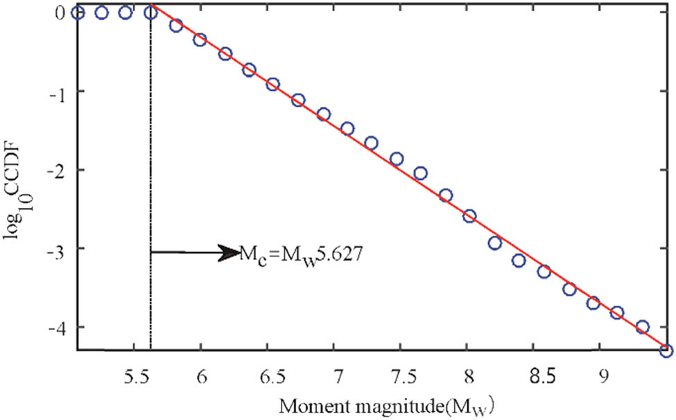
Frequency-size distribution (log linear plot) of the global earthquakes from 1960 to 2014. Earthquakes not less than M_w 5.6 are completely recorded in the ISC catalogue and can be subjected to the statistical analysis. CCDF, complementary cumulative distribution function; M_c, minimum magnitude of completeness; M_w, moment magnitude.

2.2 Heat flow data

The global HF data are obtained from National Centers for Environmental Information (NCEI), as shown in Figure 2. They are provided by the University of North Dakota and maintained by the International Heat Flow Commission (IHFC) of the International Association of Seismology and Physics of the Earth’s Interior (IASPEI). The data cover both continental and marine plates, consisting of 35,523 continental HF points and 23,013 marine points. All data are in the CSV format. They have location information; therefore, they can be located on a map.

Figure 2

Global heat flow data.

3 Research process and methods

3.1 Research process

To analyze the relationship of HF with seismicity, this research contains four parts as shown in Figure 3: (1) obtaining the data, which are already described in Section 2. (2) Dividing the global tectonically active zone into different research units. First, a tectonically active zone was extracted based on the earthquake event density (ρ). Then, the tectonically active zone was further divided based on ρ. (3) Evaluating the seismicity and HF status in each research unit. The seismic frequency-size distribution in the global tectonically active zones was analyzed, and the HF status in a unit was represented by the average HF within it. (4) Finally, analyzing the relationship of HF with the seismic frequency-size distribution. Three methods are discussed in this article, as highlighted by the light green background color in Figure 2: how to extract and divide tectonically active zones, how to evaluate seismic frequency-size distribution, and how to analyze the relationship between HF and seismicity based on the geographical detector method.

Figure 3

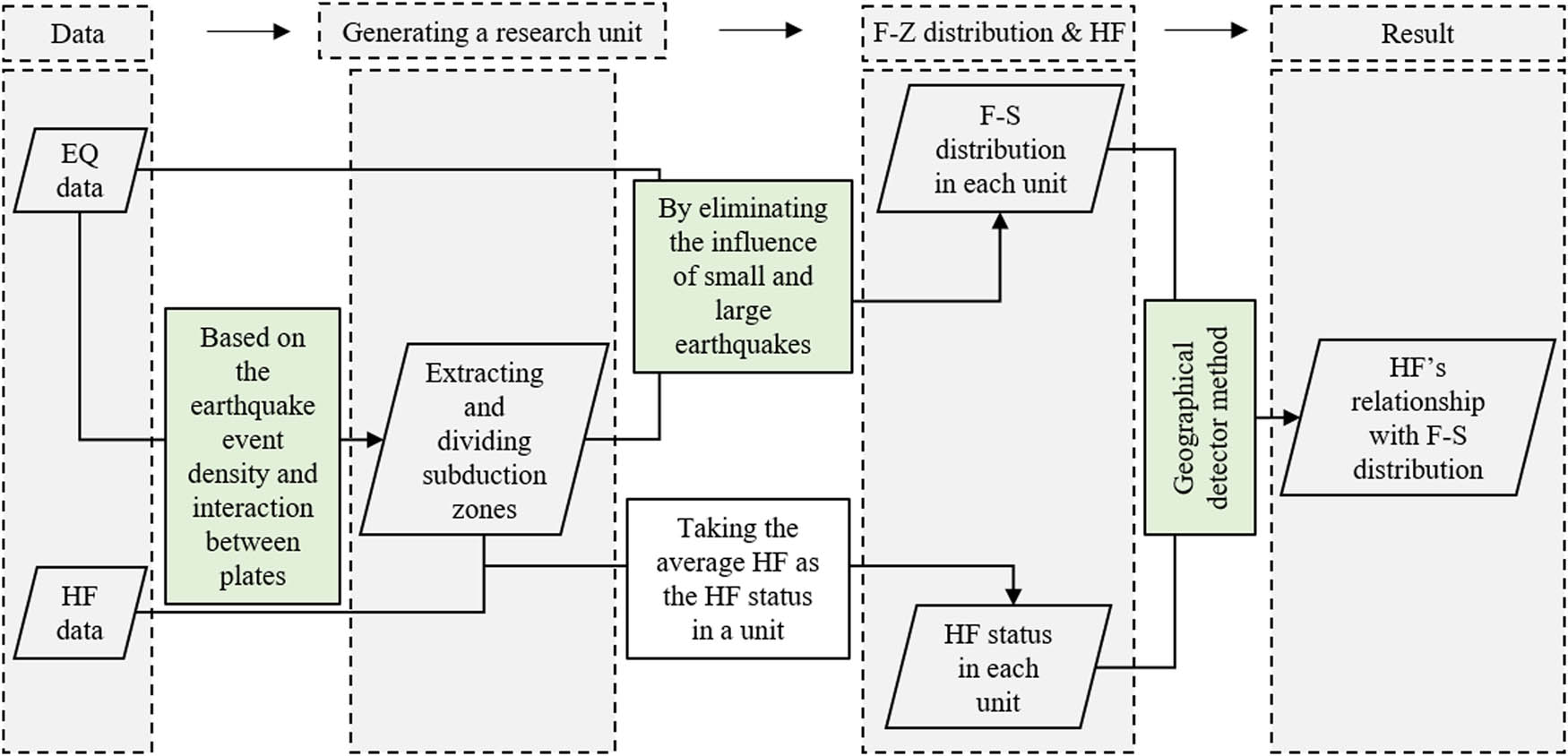
Research process for exploring the relationship between heat flow and seismicity. The process consists of 4 parts: obtaining the data source, generating a research unit, evaluating the seismicity and heat flow, and exploring the heat flow’s relationship with seismicity. The three methods are highlighted in light green. EQ, earthquake; HF, heat flow.

3.2 Research methods

3.2.1 Generating a research unit

To evaluate the spatial heterogeneity of seismicity, this article generated a research unit by dividing the global tectonically active region. A total of 71 zones were obtained, and two steps were needed for this result. First, we extracted 8 tectonically active zones in the global based on the earthquake event ρ, which is shown as S1–S8 in Figure 4(a). This study was based on earthquakes striped and aggregated distribution in the tectonically active region, as shown in Figure 4(b) and (c), respectively, corresponding to the result of interactions among plates. Usually, the earthquake distribution shows that, for interaction plates, the earthquakes become more discrete along the arrow direction as shown in Figure 4(b), which represents an increasing distance from the interface of two plates. On the basis of a certain ρ value, we outlined the strip shape of the region. Then, we separated the region of triple junction plates based on data aggregation. Earthquakes show aggregation between any two plates, as shown in Figure 4(c). Usually, there is a gap among the triple junction plates, which is indicated by black lines in the figure. Finally, we could separate the joint part of triple junction plates based on the gap.

Figure 4

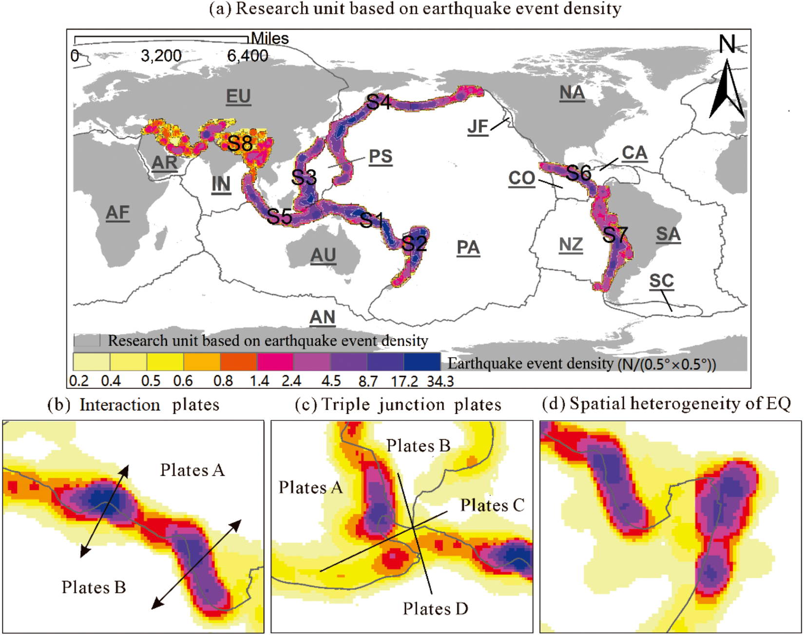
Research unit and some characteristics of earthquake distribution. (a) Research unit divided by the earthquake event density and 15 plates. S1–S8 are tectonically active zones; 71 research units are extracted by 10 density levels shown with yellow to purple. (b) Earthquake distribution between interaction plates. Usually, earthquakes are gradually dispersed with the increasing distance from the interface of plates, as shown with arrows. (c) Earthquake distribution among triple junction plates. The interaction regime from one interaction to another presents gaps shown by the black lines. (d) The detail of spatial heterogeneity of earthquake event distribution. EQ, earthquake.

The detailed extraction and division processes were as follows: (1) computing the earthquake event density based on a 0.5° × 0.5° grid. ρ is the average earthquake number in a grid. (2) Outlining the strip shape of the zones based on ρ > 0.2. ρ = 0.2 was a suitable value for distinguishing the aggregation between interaction plates and heterogeneous among interaction plates. (3) Separating the joint part of triple junction plates based on earthquake aggregation. Here, ρ was taken as an important parameter for evaluating the aggregation, and then, it was used for detecting the gap. When ρ monotonically decreased with the increasing distance from the interface among triple junction plates, the earthquakes belonged to the same zone. Otherwise, they should be divided into different zones. Finally, the tectonically active region had been divided into 8 zones.

Second, we further divided the 8 zones into 71 zones based on different ρ levels, as shown with polygon regions expressed with different colors in Figure 4(a). This work was based on ρ presented spatial heterogeneity on a fine scale, as shown in Figure 4(d). The light yellow areas corresponded to the minimum density, and the deep purple areas corresponded to the maximum density. The ρ levels were divided by the geometrical interval method. The specific benefit of the method is that it works reasonably well on data that are not distributed normally [23]. Then, the ρ was divided into 10 levels. The corresponding 8 zones in step 1 were divided into fine zones. To accurately estimate β-values, this article extracted only zones in which the earthquake count is more than 200. Finally, 71 zones remained.

3.2.2 Evaluating seismicity

We would evaluate the seismicity based on the G–R law. This G–R law is expressed as follows: log N = a – b·M, where N is the cumulative number of events, M is the magnitude, and “b” is a constant that describes the seismic frequency-size distribution. Furthermore, the logarithmic relationship between the magnitude and the seismic moment (energy) is log E ∝ 1.5 M, where the symbol ∝ stands for proportional to. The G–R equation indicates that the earthquake magnitude satisfies a logarithmic transformation of seismic moment (energy) E. Therefore, the G–R relation can be rewritten as log N = α – β·log E, where β = 2·b/3 [24,25,26]. Similar to b, β is the relative size distribution of the seismic moment (energy). With an increasing β-value, the decay rate of seismic counts moving from large to small increases. At the same time, the proportion of large earthquakes decreases.

Here, we used the β-value to evaluate seismicity. Some points need to be considered when fitting β-values. Although the earthquake size is complete in the global area, the result may not be in a unit. Therefore, the relationship between M_w and CCDF in all sizes might not be a straight line in a unit. Usually, there exists a turning around at small earthquakes and a tailing with large earthquakes. These features could be a result of small earthquakes being difficult to detect large earthquakes either undergoing another fracture mechanism or being incompletely recorded.

Therefore, in this article, the β-value was evaluated after eliminating the influence of small and large earthquakes. In other words, this parameter was based on only medium-strong earthquakes. This research recognized these earthquakes based on β-value robustness. The main idea was that after eliminating small and large earthquakes, the estimated β-values in different magnitude ranges are nearly the same. However, they might have large fluctuations due to the existence of large and small earthquakes. In this article, we used a sliding window to detect robustness. With a fixed-size window sliding across small to large earthquakes, a series of β-values would be produced. By constraining the confidence interval, we selected β-values produced by medium-strong earthquakes. The detailed process is shown in Figure 5. First, we used a sliding window to fit β-values in different ranges. Earthquakes in each window produced a β-value. Within a window, the least-squares method was used for the fitting, the earthquake count was set as 200, and the sliding step was 1 earthquake event. Then, we selected β-values falling in the 90% confidence interval. Finally, we took the average β-values in a unit as the seismicity.

Figure 5

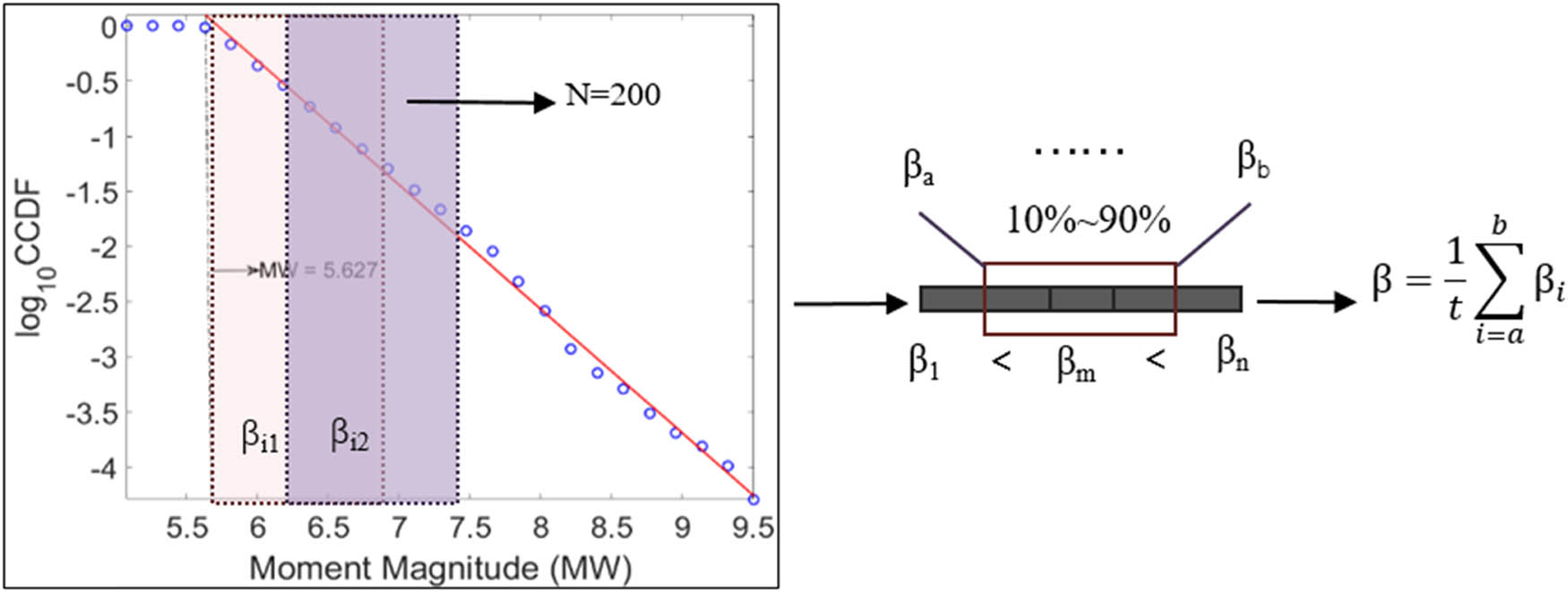
Process of fitting β-values. The fitting is based on an overlapping sliding window (purple and pink rectangles), with each containing 200 events. A series of β-values is obtained, and the β-value in a zone is the average of β-values falling in a 90% confidence interval. CCDF, complementary cumulative distribution function; t, number of β-values located between β_a and β_b.

3.2.3 Geographical detector method

The geographical detector method is based on the hypothesis that if an independent variable (HF) has some relationship with a dependent variable (β-value), and heterogeneity of the dependent variable is more evident after being constrained by the independent variable. As mentioned earlier, the method is well suited for analyzing nonlinear relationships with variance [27]. Variance is used for assessing the heterogeneity. Constrained could also be described as a process of modularization. If A is constrained by B, then A is divided into several parts by B. For example, in this article, if β-value is constrained by HF, then the β-value is allocated to the corresponding HF interval by some rules (e.g., spatial position). The independent variable should be categorical. In this article, HF is the categorical variable. The relationship of HF with seismicity is determined by evaluating whether the β-value is more homogeneous after being constrained by HF. In other words, if HF has some impact on β-value, then the variance of β-value is more evidence after being constrained by HF. The principle is described in Figure 6. The figure on the left shows the principle of this method. The formula on the right shows how the correlation degree is calculated, where y is the β-value falling in a category of HF, σy² is the y variance, N_y is the count of y, L is the count of HF type, σ² is the β-value variance in an unconstrained state, and N is the count of β-value. q is the influence degree. The q value close to 1 means X shows a good relationship with Y, and the q value close to 0 means X has almost no relationship with Y.

Figure 6

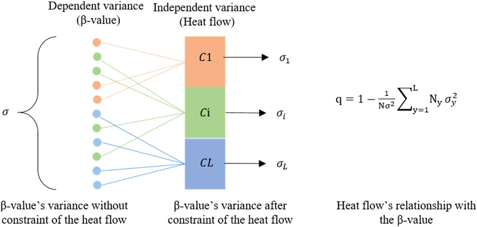
Principles of the geographical detector method and calculation of the correlation degree. The method evaluates the independent variable’s relationship with the dependent variable (dots) according to the enhancement in the dependence variable’s variance after being constrained by the independent variable. Constrained could also be described as a process of modularization. If A is constrained by B, then A is divided into several parts by B. The evaluation equation is shown in the figure. q, correlation degree.

4 Spatial heterogeneity of heat flow and seismicity

4.1 Heat flow

Before analyzing the HF’s relationship with seismicity, we first present the spatial heterogeneity of HF. This article takes the average HF as the HF status in a unit, and the spatial heterogeneity of HF is shown in Figure 7. The average HF value is shown with a color gradient. Light green represents the minimum, and deep red represents the maximum. The spatial pattern of the average HF in the figure shows that the whole northwest Pacific Ocean is hot and that the southwest Pacific Ocean is cold. Among the interaction plates with significant HF heterogeneity (e.g., S3/S4/S5), the HF spatial heterogeneity is similar to its already discovered distribution [28].

Figure 7

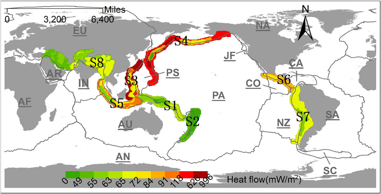
Spatial heterogeneity of heat flow in global tectonically active zones. The heat flow in each zone is the average value.

4.2 Seismicity

Based on the evaluation method mentioned in Section 3.2.2, the spatial heterogeneity of seismicity is shown in Figure 8. The seismicity exhibits heterogeneity either between interplate zones or within interplate zones. It ranges between 0.57 and 0.83, corresponding to the color gradient. Between interplate zones, heterogeneity is especially evident between Tonga (S2) and South America (S7). The β-values in Tonga are generally the highest overall, but in SA they are generally the lowest overall. Within the interplate zones, the frequency size of a medium-strong earthquake also presents heterogeneity, for example, S5 and S6. Usually, the β-value gradually varies with the increasing distance from interaction faces. In S5 and S6, the β-value decreases with the increasing distance from the interaction faces. The implication is that strong earthquakes are more concentrated with the increasing distance from interaction faces.

Figure 8

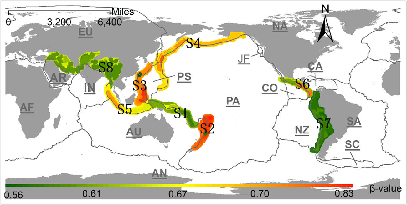
Spatial heterogeneity of seismicity. The β-values in S2 are generally the highest, which means that medium earthquakes are more concentrated in S2. The case is opposite in S7. In S5 and S6, strong earthquakes are more concentrated with the increasing distance from interaction faces.

5 Heat flow’s relationship with seismicity

According to the spatial pattern of HF and seismicity, the seismicity does not present a significant linear relationship with HF. For example, in Figure 7, the HF spatial distribution is shown: HF in Tonga (S2) is generally the lowest overall, NW-PA/PS (S3/S4) is higher, and other zones are in between. However, a zone with high HF is not necessarily one with a high (or low) β-value. For example, HF in SA (S7) is between the highest and lowest, but its β-value is the lowest. This result could be that the seismicity is related to other various complex factors besides HF [26,29]. Different impacting factors would have different impacting degrees on seismicity. However, the impacting degree would not be obvious for anyone. In this case, the geographical detector method would be a good choice to analyze the relationship between HF and seismicity.

By using the geographical detector method, this part detects the relationship of HF with seismicity. First, the HF is divided into 10 categories according to the percentile of the HF value. The percentile range is from 0 to 100, and the step size is 10. HF falling in certain percentile intervals would be classified into the same category. For example, HF values within [627 996], which fall in the 90–100% percentile interval, are category 1, HF values within [119 626], which fall in the 80–90% percentile interval, are category 2, and so on. If HF has a relationship with seismicity, then variation in the β-value would increase after being constrained by HF. Then, we detect the change in variation according to the formula shown in Figure 6.

Based on the 71 zones, the relationship between HF and β-values is shown in Figure 9. Figure 9 shows the β-value distribution in different HF intervals, where the x-axis is the HF value located at different percentile points, and the y-axis is the β-value distribution that falls in an HF interval. The distribution indicates that HF might have different relationships with the β-value based on the HF interval. Thus, in addition to the overall influence, we detect the relationship of HF with the β-value in constrained intervals. The result is also shown in Figure 9, where q is the correlation degree. After setting different split points, we find that when HF = 84 mW/m²q in either interval is more significant, the relationship can be better described. Finally, we select HF = 84 mW/m² as the split point.

Figure 9

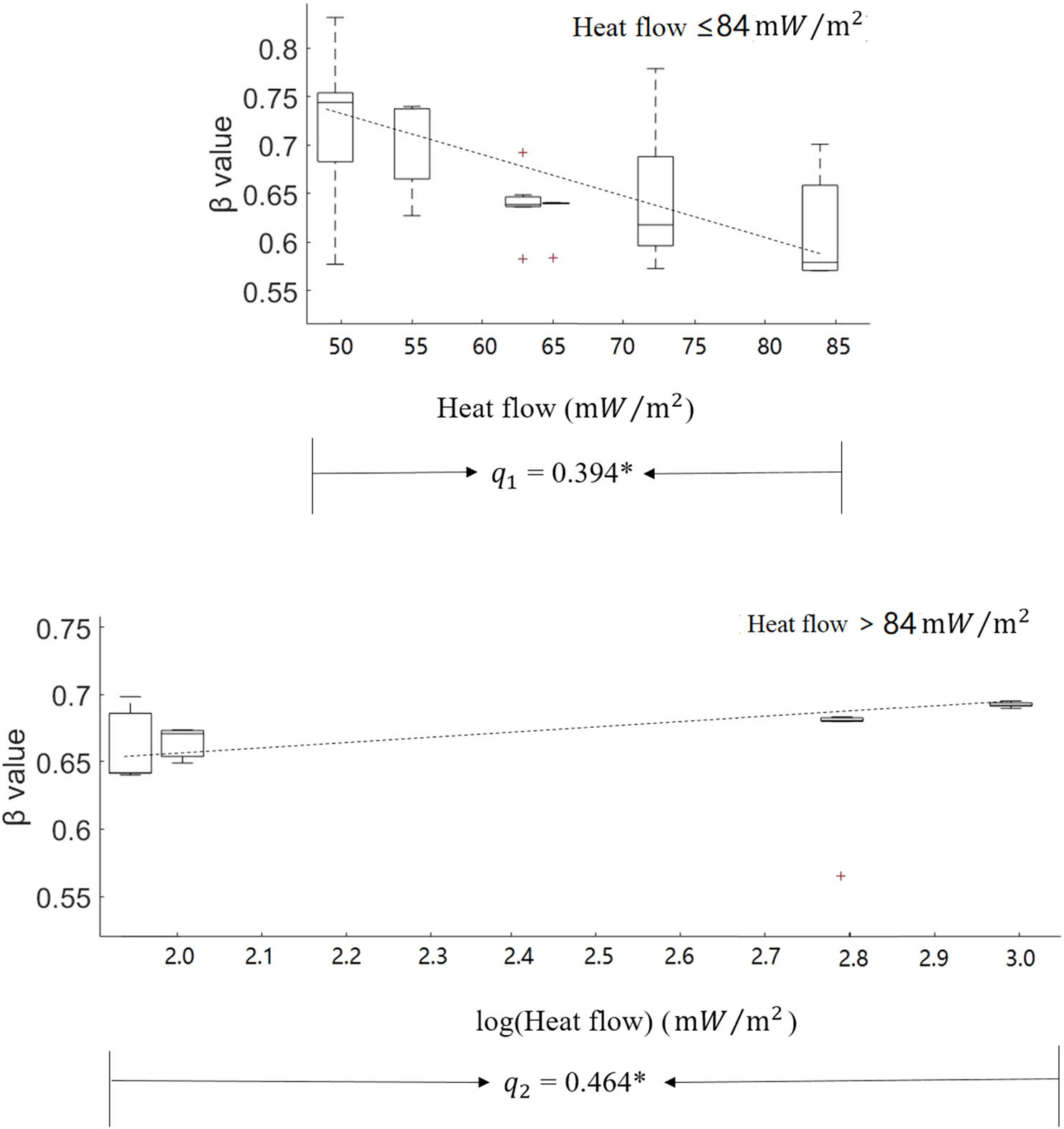
Relationship between heat flow and seismicity. The seismicity distribution (y-axis) in different heat flow intervals (x-axis) is shown. The result indicates that their correlation degree presents a significant difference based on the split point HF = 84 Mw/m². q₁, correlation degree when HF < 84 Mw/m²; q₂, correlation degree when HF > 84 Mw/m². * Correlation degree is significant. Red crosses represent outliers based on the boxplot.

The result indicates that over the entire HF value range, HF has a significant relationship with seismicity, with a correlation degree of 0.395. However, after constraining the HF interval, the relationship is more significant, and the related mechanisms could be different. With the split point HF = 84 mW/m², when HF < 84 mW/m², HF has a negative relationship with seismicity, and the correlation degree is 0.394; when HF > 84 mW/m², HF has a positive relationship with seismicity, and the correlation degree is 0.464. Furthermore, the correlation degrees are all significant.

6 Discussion

This study shows that HF has a dual relationship with seismicity. There is an interval effect between HF and the β-value, and the HF value at the critical point of the interval is HF = 84 mW/m². This critical point is similar to the average HF (87 mW/m²) in the global data [30].

When HF < 84 mW/m², HF correlates negatively with the β-values, and the correlation degree is 0.394. The reason why the β-value decreases with the increasing HF in the lower value interval is probably that buoyant is a primary control on the stress state and earthquake size distribution. Large earthquakes occur more frequently in subduction zones with younger slabs that are more buoyant [31]. Zones with a high ratio of large earthquakes would correspond to low β-value. Therefore, a high HF value corresponds to a low β-value. Besides, Zhan [13] also shows that the β-value of deep earthquakes is strongly temperature dependent, high in cold slabs, and low in a warm slab.

However, when HF > 84 mW/m², HF correlates positively with the β-values, and the correlation degree is 0.464. In the higher value interval, an increase of HF decreases the viscosity of the rock plate, resulting in a high strain rate and low stress [32,33]. Previous studies have also shown that β-value is related to the level of stress. The low stress would weaken the earthquake events by decreasing the locking between the subducting slab and the overlapping plate [34]. The areas with higher stress levels have lower β-values, while the areas with lower stress levels have higher β-values [35,36,37,38]. Therefore, in this interval, the high HF would correspond to the low stress and then the high β-value.

7 Conclusions

Seismicity is an important part of the seismic hazard assessment. The study of related factors leading to seismic activities is helpful to detect the accuracy and timeliness of seismic hazard assessment. In this article, we use the geographical detector method to analyze the complex relationship of HF with seismicity in global tectonically active zones. The β-value is used to assess seismicity. The results show that HF shows different relationships with seismicity based on different intervals. When HF < 84 mW/m², HF correlates negatively with the β-value, and its correlation degree with the β-value is 0.394. Within this interval, slabs with high HF are more buoyant, which enhances interface coupling between plates. The stress level in the rock plate is increased, and the magnitude of the earthquake that occurs at this time is also large, so the high HF value corresponds to a low β-value. When HF > 84 mW/m², HF correlates positively with the β-value, and the correlation degree with the β-value is 0.463. Within this interval, increasing HF decreases the viscosity of the rock plate and also the stress levels. The magnitude of the earthquake that occurs at this time is relatively small, which corresponds to a high β-value. Therefore, a high HF corresponds to a high β-value in this case.

However, there are still some limitations in this study. This article uses tectonically active regions to perform the analysis and has not considered the different tectonic features formed in different backgrounds. This would induce the complexity of geographical factors on seismicity and might weaken the correlation degree between HF and β-value. In the future, the analysis of different types of tectonic features should be considered separately.

Acknowledgments

This work was supported by the National Natural Science Foundation of China (41771537).

Author contributions: Conceptualization, CXC and JY; Methodology, JY and CXC; Formal Analysis, CH; Writing-Original Draft Preparation, JY; Writing-Review and Editing, CH; Supervision, CXC and SS; Funding acquisition: CXC. All authors have read and agreed to the published version of the manuscript.

References

[1] Klügel JU. Seismic hazard analysis—Quo vadis? Earth-Sci Rev. 2008;88(1–2):1–32. 10.1016/j.earscirev.2008.01.003.Suche in Google Scholar

[2] Schorlemmer D, Wiemer S, Wyss M. Variations in earthquake-size distribution across different stress regimes. Nature. 2005;437(7058):539. 10.1038/nature04094.Suche in Google Scholar PubMed

[3] Gulia L, Wiemer S. The influence of tectonic regimes on the earthquake size distribution: A case study for Italy. Geophys Res Lett. 2010;37:L10305. 10.1029/2010GL043066.Suche in Google Scholar

[4] Main I. Statistical physics, seismogenesis, and seismic hazard. Rev Geophysics. 1996;34(4):433–62. 10.1029/96RG02808.Suche in Google Scholar

[5] Kagan YY, Jackson DD. Earthquake rate and magnitude distributions of great earthquakes for use in global forecasts. Geophys J Int. 2016;206(1):630–43. 10.1093/gji/ggw161.Suche in Google Scholar

[6] Riguzzi F, Crespi M, Devoti R, Doglioni C, Pietrantonio G, Pisani AR. Geodetic strain rate and earthquake size: New clues for seismic hazard studies. Phys Earth Planet Inter. 2012;206:67–75. 10.1016/j.pepi.2012.07.005.Suche in Google Scholar

[7] Kalyoncuoglu UY, Elitok Ö, Dolmaz MN. Tectonic implications of spatial variation of b-values and heat flow in the Aegean region. Mar Geophys Res. 2013;34(1):59–78. 10.1007/s11001-013-9174-8.Suche in Google Scholar

[8] Yang J, Cheng C, Song C, Shen S, Zhang T, Ning L. Spatial-temporal distribution characteristics of global seismic clusters and associated spatial factors. Chin Geogr Sci. 2019;29(4):614–25. 10.1007/s11769-019-1059-6.Suche in Google Scholar

[9] Srivastava K. Modelling the variability of heat flow due to the random thermal conductivity of the crust. Geophys J R Astronomical Soc. 2005;160(2):776–82. 10.1111/j.1365-246X.2005.02456.xSuche in Google Scholar

[10] Yu Q, Ren Z, Wang B, Zheng W, Tao N. Geothermal field and deep thermal structure of the Tianshan-Altun region. Geol J. 2018;53:237–51. 10.1002/gj.3202.Suche in Google Scholar

[11] Liu B, Li SZ, Suo YH, Li GX, Dai LM, Somerville ID, et al. The geological nature and geodynamics of the Okinawa Trough, Western Pacific. Geol J. 2016;51:416–28. 10.1002/gj.2774.Suche in Google Scholar

[12] Papadakis G, Vallianatos F, Sammonds P. Non-extensive statistical physics applied to heat flow and the earthquake frequency–magnitude distribution in Greece. Phys A: Stat Mech its Appl. 2016;456:135–44. 10.1016/j.physa.2016.03.022.Suche in Google Scholar

[13] Zhan Z. Gutenberg–Richter law for deep earthquakes revisited: A dual-mechanism hypothesis. Earth Planet Sci Lett. 2017;461:1–7. 10.1016/j.epsl.2016.12.030.Suche in Google Scholar

[14] Phillips JD. Sources of nonlinearity and complexity in geomorphic systems. Prog Phys Geography: Earth Environ. 2003;27(1):1–23. 10.1191/0309133303pp340raSuche in Google Scholar

[15] Cheng CX, Shi PJ, Song CQ, Gao JB. Geographic big-data: A new opportunity for geography complexity study (in Chinese). Acta Geogr Sin. 2018;73(8):1397–406. 10.11821/dlxb201808001.Suche in Google Scholar

[16] Shen S, Ye SJ, Cheng CX, Song CQ, Gao JB, Yang J, et al. Persistence and corresponding time scales of soil moisture dynamics during summer in the Babao River Basin, Northwest China. J Geophys Res: Atmos. 2018;123(17):8936–48. 10.1029/2018JD028414.Suche in Google Scholar

[17] Zhang T, Shen S, Cheng CX, Song CQ, Ye SJ. Long-range correlation analysis of soil temperature and moisture on A’rou Hillsides, Babao River Basin. J Geophys Res: Atmos. 2018;123(22):12,606–20. 10.1029/2018JD029094.Suche in Google Scholar

[18] Wang JF, Li XH, Christakos G, Liao YL, Zhang T, Gu X, et al. Geographical detectors-based health risk assessment and its application in the neural tube defects study of the Heshun Region, China. Int J Geogr Inf Sci. 2010;24(1):107–27. 10.1080/13658810802443457.Suche in Google Scholar

[19] Turcotte DL, Malamud BD. Landslides, forest fires, and earthquakes: Examples of self-organized critical behavior. Phys A: Stat Mech its Appl. 2004;340(4):580–9. 10.1016/j.physa.2004.05.009.Suche in Google Scholar

[20] de Arcangelis L, Godano C, Grasso JR, Lippiello E. Statistical physics approach to earthquake occurrence and forecasting. Phys Rep. 2016;628:1–91. 10.1016/j.physrep.2016.03.002.Suche in Google Scholar

[21] Storchak DA, Giacomo Di, Bondár D, Engdahl I, Harris ER, Lee J, et al. Public release of the ISC-GEM global instrumental earthquake catalogue (1900–2009). Seismol Res Lett. 2013;84(5):810–5. 10.1785/0220130034.Suche in Google Scholar

[22] Schorlemmer D, Hirata N, Ishigaki Y, Doi K, Nanjo KZ, Tsuruoka H, et al. Earthquake detection probabilities in Japan. Bull Seismol Soc Am. 2018;108(2):702–17. 10.1785/0120170110.Suche in Google Scholar

[23] Frye C. About the geometrical interval classification method. Environmental Systems Research Institute, Inc.; 2007. Online verfügbar unter https://blogs. esri. com/esri/arcgis/2007/10/18/about-thegeometrical-interval-classification-method.Suche in Google Scholar

[24] Kagan YY. Earthquake size distribution: Power-law with exponent β ≡ 1/2? Tectonophysics. 2010;490(1–2):103–14. 10.1016/j.tecto.2010.04.034.Suche in Google Scholar

[25] Bell AF, Naylor M, Main IG. Convergence of the frequency-size distribution of global earthquakes. Geophys Res Lett. 2013;40(11):2585–9. 10.1002/grl.50416.Suche in Google Scholar

[26] Cheng QM, Sun HY. Variation of singularity of earthquake-size distribution with respect to tectonic regime. Geosci Front. 2018;9(2):453–8. 10.1016/j.gsf.2017.04.006.Suche in Google Scholar

[27] Luo L, Mei K, Qu L, Zhang C, Chen H, Wang S, et al. Assessment of the geographical detector method for investigating heavy metal source apportionment in an urban watershed of Eastern China. Sci Total Environ. 2019;653:714–22. 10.1016/j.scitotenv.2018.10.424.Suche in Google Scholar PubMed

[28] Currie CA, Hyndman RD. The thermal structure of subduction zone back arcs. J Geophys Res: Solid Earth. 2006;111:B08404. 10.1029/2005JB004024.Suche in Google Scholar

[29] El-Isa ZH, Eaton DW. Spatiotemporal variations in the b-value of earthquake magnitude–frequency distributions: Classification and causes. Tectonophysics. 2014;615:1–11. 10.1016/j.tecto.2013.12.001.Suche in Google Scholar

[30] Pollack HN, Hurter SJ, Johnson JR. Heat flow from the Earth’s interior: Analysis of the global data set. Rev Geophys. 1993;31(3):267–80. 10.1029/93RG01249.Suche in Google Scholar

[31] Nishikawa T, Ide S. Earthquake size distribution in subduction zones linked to slab buoyancy. Nat Geosci. 2014;7:904–8. 10.1038/ngeo2279.Suche in Google Scholar

[32] Zaliapin I, Ben-Zion Y. A global classification and characterization of earthquake clusters. Geophys J Int. 2016;207(1):608–34. 10.1093/gji/ggw300.Suche in Google Scholar

[33] Lachenbruch AH, Sass JH. Heat flow from Cajon Pass, fault strength, and tectonic implications. J Geophys Res: Solid Earth. 1992;97(B4):4995–5015. 10.1029/91JB01506.Suche in Google Scholar

[34] Kong XC, Li S, Suo YH, Guo L, Li XY, Liu X, et al. Hot and cold subduction systems in the Western Pacific Ocean: Insights from heat flows. Geol J. 2016;51:593–608. 10.1002/gj.2802.Suche in Google Scholar

[35] Scholz CH. The frequency-magnitude relation of microfracturing in rock and its relation to earthquakes. Bull Seism Soc Am. 1968;58(1):399–415. 10.1109/IGARSS.2013.6723499.Suche in Google Scholar

[36] Mori J, Abercrombie RE. Depth dependence of earthquake frequency‐magnitude distributions in California: Implications for rupture initiation. J Geophys Res: Solid Earth. 1997;102:15081–90. 10.1029/97JB01356.Suche in Google Scholar

[37] Wiemer S, Wyss M. Mapping the frequency‐magnitude distribution in asperities: An improved technique to calculate recurrence times? J Geophys Res: Solid Earth. 1997;102:15115–28. 10.1029/97JB00726.Suche in Google Scholar

[38] Goebel W, Schorlemmer TH, Becker D, Dresen TW, Sammis G, Acoustic CG. emissions document stress changes over many seismic cycles in stick-slip experiments. Geophys Res Lett. 2013;40(10):2049–54. 10.1002/grl.50507.Suche in Google Scholar

Received: 2020-06-07

Revised: 2020-08-12

Accepted: 2020-09-21

Published Online: 2020-11-19

This work is licensed under the Creative Commons Attribution 4.0 International License.

Artikel in diesem Heft

https://doi.org/10.1515/geo-2020-0195

Schlagwörter für diesen Artikel

spatial analysis; seismicity; heat flow; geographic detector method; nonlinearity

Creative Commons

BY 4.0