Comparison of swarm intelligence algorithms for optimized band selection of hyperspectral remote sensing image
-
Ding Xiaohui
 ,
Li Yong
,
Li Yong

Abstract
Swarm intelligence algorithms have been widely used in the dimensional reduction of hyperspectral remote sensing imagery. The ant colony algorithm (ACA), the clone selection algorithm (CSA), particle swarm optimization (PSO), and the genetic algorithm (GA) are the most representative swarm intelligence algorithms and have often been used as subset generation procedures in the selection of optimal band subsets. However, studies on their comparative performance for band selection have been rare. For this paper, we employed ACA, CSA, PSO, GA, and a typical greedy algorithm (namely, sequential floating forward selection (SFFS)) as subset generation procedures and used the average Jeffreys–Matusita distance (JM) as the objective function. In this way, the band selection algorithm based on ACA (BS-ACA), band selection algorithm based on CSA (BS-CSA), band selection algorithm based on PSO (BS-PSO), band selection algorithm based on GA (BS-GA), and band selection algorithm based on SFFS (BS-SFFS) were tested and evaluated using two public datasets (the Indian Pines and Pavia University datasets). To evaluate the algorithms’ performance, the overall classification accuracy of maximum likelihood classifier and the average runtimes were calculated for band subsets of different sizes and were compared. The results show that the band subset selected by BS-PSO provides higher overall classification accuracy than the others and that its runtime is approximately equal to BS-GA’s, higher than those of BS-ACA, BS-CSA, and BS-SFFS. However, the premature characteristic of BS-ACA makes it unacceptable, and its average JM is lower than those of other algorithms. Furthermore, BS-PSO converged in 500 generations, whereas the other three swarm-intelligence based algorithms either ran into local optima or took more than 500 generations to converge. BS-PSO was thus proved to be an excellent band selection method for a hyperspectral image.
1 Introduction
A hyperspectral remote sensor scans ground objects with a spectrum covering visible to infrared region, and generally records the spectral signature with hundreds of narrow bands, thus bringing great opportunities for the quantitative analysis of remote sensing. However, the hyperspectral imagery (HSI) poses a major challenge for data storage, management, processing, and analysis because of its massive data quantities and the serious data redundancy among the bands with high correlations [1]. For example, the “Hughes phenomenon” will be faced when classifying land use/cover types with HSI, where a limited number of training samples are usually collected [2]. It is, therefore, of paramount importance, to reduce the data redundancy and data dimension, so as to facilitate the analysis of hyperspectral remote sensing. Generally, dimensionality reduction methods can be divided into two categories: feature extraction and feature selection. The feature extraction techniques include unsupervised approaches, such as principal component analysis (PCA) and independent component analysis (ICA) [3,4,5], and supervised approaches, such as Fisher’s linear discriminant analysis (LDA) [6]. But all these feature extraction methods are not suitable for dimensionality reduction of HSI [7]. For example, PCA, which often uses an ideal projection method to linearly transform the original high-dimensional data into a low-dimensional feature space, is incapable of drawing distinctions between patterns [8]; ICA assumes that the observed signals are statistically independent of each other and that the observed signal vector is a linear mixture of these separate independent components, but such a decorrelation assumption cannot be satisfied with HSI [9]; LDA, which is similar to PCA, fails when the class-conditional distributions are not Gaussian [10]. In recent years, because of its good performance on the preservation of primitive physical interpretability [11], feature selection has received increasing attention from researchers in the field of remote sensing. This type of method tries to pick the most representative subset from a large number of HSI features to maintain acceptable classification accuracy [12]. The general process of feature selection consists of the following basic steps: the generation procedure, evaluation function, stopping criterion comparison, and validation procedure [13]. The generation procedure searches for a feature subset for evaluation, which is the basis of the feature selection model. To date, many subset generation procedures have been proposed in relevant studies, which can be generally classified into three types: full search, heuristic search, and random search. Breadth-first search (BFS), which is a typical full-search method, is unpractical, because it enumerates exhaustively all of the possible combinations of features and results in a high time complexity. The heuristic search method reduces the search space with heuristic information, whose order of the search space is quadratic in terms of the number of features. Greedy algorithms (e.g., sequential forward selection (SFS), sequential backward selection (SBS)), plus-L minus-R selection (LRS), sequential floating forward selection (SFFS), and sequential floating backward selection (SFBS)) are widely used heuristic search methods [14,15]. Generally, SFFS and SFBS have better performance than others that are similar [14]. The SFFS-based feature selection algorithm selects the optimal feature subset in a two-stage selection process. Firstly, a new feature is appended to the previously selected feature subset, and secondly, a feature is discarded to achieve the maximum value of the objective function [16,17].
The ant colony algorithm (ACA) is an emerging heuristic search algorithm, and its effectiveness has been proved in the field of HSI band selection [18]. The random search methods start the procedure with some of the feature subsets initialized randomly. Typical random search methods including simulated annealing (SA), genetic algorithm (GA), particle swarm optimization (PSO), and the clone selection algorithm (CSA) have been widely used in feature selection [19,20]. Among the above-mentioned three types of generation procedures, ACA, GA, PSO, and CSA are typical swarm intelligence algorithms, which often have excellent ability for self-organization, self-learning, or self-memory.
Optimal feature subset selection for HSI is a typical NP-hard problem [12], which should be solved with a proper search procedure [21]. Thus, swarm intelligence algorithms, such as ACA, GA, PSO, and CSA, have been widely employed in the optimized feature selection of the original hyperspectral data [22]. Many studies have shown that the swarm intelligence algorithms have better performance than other search algorithms in HSI feature selection. The performance of ACA was compared with that of SFFS and was also compared with that of GA [1,8,13,23]. Zhong et al. compared CSA and its improved version with SFS for HSI band selection [24]. The performance of PSO for feature selection has also been compared with those of GA, SFS, and other search algorithms [15,25,26]. However, the performance of swarm intelligence algorithms for HSI feature selection has not been investigated systematically.
In this study, the typical swarm intelligence algorithms were used for selecting the optimal band subset from HSI, and their performance in terms of overall classification accuracy and average runtime was compared and analyzed. To make a comprehensive comparison, the SFFS, one of the most effective greedy search methods, was also included as a benchmark comparator to further verify the effectiveness of the swarm intelligence algorithms. Thus, a total of five algorithms (including ACA, GA, PSO, CSA, and SFFS) were compared on two public hyperspectral datasets (The Indian Pines and Pavia University datasets). The motivation of this paper is to provide a reference for the selection of dimensional reduction methods and algorithm improvement to guide future research.
2 Materials and methods
2.1 Data source
In our experiment, two public hyperspectral datasets were used to compare the performances of the above-mentioned algorithms. The first site covered by mixed vegetation is located in the Indian Pines test site in northwest of Indiana (Indian Pines dataset). The second site is an urban site over the Pavia University, northern Italy (Pavia University dataset).
The Indian Pines dataset (Indian dataset) was acquired by the airborne visible/infrared imaging spectrometer (AVIRIS) sensor on June 12, 1992 (Figure 1a). The imagery is composed of 224 bands, with a wavelength ranging from 0.4 to 2.5 µm. The 10 nm spectral resolution provides refined discrimination among similar land covers. After removal of the bands that were seriously influenced by moisture absorption, there were 200 bands remaining in the Indian dataset. Thus, the size of the dataset is 145 × 145 × 200. The ground truth for this area consisted of 16 land cover types (Figure 1b). As commonly used in previous literature [27,11], nine land cover types that have enough samples of ground truth were chosen from the 16 categories in this experiment. The training and testing samples of these classes, derived from the ground truth map, are shown in Table 1.
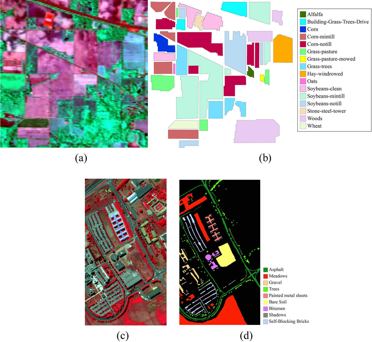
(a) The Indian dataset; (b) ground truth for the same area; (c) the Pavia dataset; (d) ground truth for the same area of Pavia University.
Land cover classes and the number of training and testing samples in the Indian dataset
| Land cover type | No. of training samples | No. of test samples | Total |
|---|---|---|---|
| C1. Corn-min | 415 | 415 | 830 |
| C2. Corn-notill | 714 | 714 | 1,428 |
| C3. Grass/pasture | 241 | 242 | 483 |
| C4. Grass/tree | 365 | 365 | 730 |
| C5. Hay-windrowed | 239 | 239 | 478 |
| C6. Soybeans-clean | 296 | 297 | 593 |
| C7. Soybeans-min | 1,227 | 1,228 | 2,455 |
| C8. Soybeans-notill | 486 | 486 | 972 |
| C9. Woods | 632 | 633 | 1,265 |
| Total | 4,615 | 4,619 | 9,234 |
The original Pavia University dataset (Pavia dataset) with 340 × 610 pixels was gathered by the reflective optics system imaging spectrometer (ROSIS) sensor in 2002 (Figure 1c). The dataset contains 115 bands over 0.43–0.86 µm range of spectrum. The high spatial resolution of 1.3 m per pixel aims to avoid a high fraction of mixed pixels. The preprocessed dataset has only 103 bands after removing water absorption and low signal-to-noise ratio bands (Figure 1c). In total, nine land cover types were identified (Figure 1d). The training and testing samples of these classes, derived from the ground truth map, are shown in Table 2.
Land cover classes and the number of training and testing samples in the Pavia dataset
| Land cover type | No. of training samples | No. of test samples | Total |
|---|---|---|---|
| C1. Asphalt | 3,315 | 3,316 | 6,631 |
| C2. Meadows | 9,324 | 9,325 | 18,649 |
| C3. Gravel | 1,049 | 1,050 | 2,099 |
| C4. Trees | 1,532 | 1,532 | 3,064 |
| C5. Painted metal sheets | 672 | 673 | 1,345 |
| C6. Bare soil | 2,514 | 2,515 | 5,029 |
| C7. Bitumen | 665 | 665 | 1,330 |
| C8. Shadows | 473 | 474 | 947 |
| C9. Self-blocking bricks | 1,841 | 1,841 | 3,682 |
| Total | 21,386 | 21,391 | 42,776 |
2.2 Optimal band selection
In this study, we employed the swarm intelligence algorithms as the search processes to select bands from the original HSI to constitute the band subsets. The general algorithm flow diagram is shown in Figure 2. For convenience, solutions of these search processes are defined in a binary form. Intelligent agents of the swarms are initialized as a population of binary strings, the length of each string being equal to the number of bands of the original HSI (Figure 3). In a binary string, a value of 1 at position i means that the ith band is included in the iteration process, whereas a value of 0 indicates its absence. The binary string with M “1” characters denotes M bands are selected by the Intelligent agents.

Flow diagram for selection of optimized band subset based on a swarm intelligence algorithm.
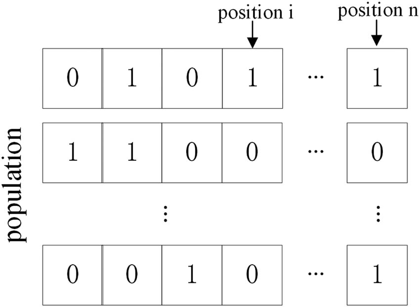
Method of encoding the solutions.
To evaluate the search results of the swarm intelligence algorithms, a reasonable objective function is also necessary. Jeffreys–Matusita distance (JM) is one of the best class separability measures for multiclass problem [28]. The JM distance between two classes ch and ck (Jh,k) can be calculated by the following equation:
where r is a d-dimensionality feature vector (the selected band subset has d bands),
where Bh,k is the Bhattacharyya distance between class ch and ck, and it can be calculated as per the following equation.
Here,
In this study, we employed the average JM among all of the classes as the criterion function to evaluate the results of the band subset selections [23]. The larger the average JM between different classes is, the better the solution will be. The average JM can be calculated as:
where
2.2.1 ACA band selection algorithm (BS-ACA)
ACA, an artificial model inspired by the foraging behavior of an ant colony in nature, was first proposed in the late 1990s [29,30]. ACA solves the optimization problem by way of stigmergy, which is an indirect information transfer among ants [31]. For convenience, we used a fully connected undirected weighted graph G = 〈B, E〉 to represent the search space of ACA-based band selection algorithm. In this graph, the elements of B indicate the graph nodes and
where ρ is a volatility coefficient that controls the volatilization rate of the pheromone.
where Norm() is an operator that normalizes its argument.
When the ant reaches
where α denotes the rate of information accumulation in the movement of the ants and β is the heuristic coefficient.
The BS-ACA is realized with the following steps [23]:
Step 1: Initialize the ant colony and the parameters, including N, Q, ρ, α, β, λ and the number of iterations T.
Step 2: Calculate the JM of ant k (k = 1), and obtain the probability that ant k will reach the candidate band set.
Step 3: Select the next band by roulette wheel selection, and repeat Step 2 until M bands are selected.
Step 4: Set k = k + 1, and repeat Steps 2 and 3 until k = N.
Step 5: Update the pheromone concentration on the route according to equation (5).
Step 6: Repeat Steps 2–5 until the iteration count reaches the user-specified number, and obtain the best band combination.
2.2.2 BS-CSA
The artificial immune system is a metaphor of an animal’s immune system. Clone selection is one of the well-known theories that effectively explain the immunity phenomenon [33]. CSA-based band selection algorithm was designed according to the clone selection theory. The objective function (JM) represents the antigen, the solution set of the specific problem denotes the population of antibody (Ab), and the value of the objective function is employed to evaluate the affinity of the solution (i.e., Ab). After the proliferation, mutation, and selection operations, the maximum affinity will approach stabilization (i.e., affinity maturation). The probability of mutation of the ith Ab (Pi) is inversely proportional to the affinity and can be calculated by equation (8).
where α is a variable coefficient, fi denotes the affinity of the ith Ab, and
The BS-CSA is designed with the following steps [34]:
Step 1: Initialize BS-CSA. The AB is generated randomly, and the parameters, including the size of the population (N) and α, are initialized.
Step 2: Calculate the affinity of AB according to equation (1).
Step 3: Select the k highest-affinity antibodies from AB to compose the new antibody population
where round() is an operator that rounds its argument toward the closest integer.
Step 4: Clone the members of
where
Step 5: Each Ab in
Step 6: Calculate the affinity of
Step 7: In order to increase the diversity of the antibody population, d antibodies are produced randomly to replace the d lowest-affinity antibodies in
Step 8: When the BS-CSA iteration count reaches the user-specified number, stop the execution of the algorithm and obtain the optimal band subset. Otherwise, return to Step 2.
2.2.3 BS-PSO
Inspired by the foraging behavior of a bird flock, the PSO was proposed [35]. A bird in the flock is regarded as a particle that represents a potential solution of the optimization problem. The particles move through the n-dimensional problem search space and search for the optimal or good enough solution. The particle broadcasts its current position to the neighboring particles. Here xi, defined by equation (12), is used to represent the position of the ith particle. The position change of each particle (as illustrated by Figure 4), defined as equation (13), is relative to its changing rate (i.e., velocity, denoted by ν).
Here, i = {1, 2,…, N}, where N is the size of the particle population.
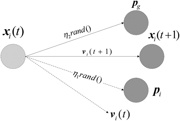
Direction of a particle’s flight.
The velocity of the particle is adjusted as follows: according to the difference between the best position found by its neighbors (
where
The selection of the optimal band subset is a discrete optimization problem, and the position xidcan be updated according to equation (15):
According to the proposed PSO-based band selection algorithm [28], the BS-PSO is designed, with the average JM distance as the objective function. The flow of BS-PSO is as follows:
Step 1: Initialize the particle population, and set the parameters, including N,
Step 2: Calculate the JM of each particle, and obtain the best optimal position of each particle and the best optimal position of the population.
Step 3: Update the velocity and position of each particle according to equations (14) and (15), respectively.
Step 4: Recalculate the JM of each particle, and update the best positions found by the particle and its neighbors when the JM has been improved.
Step 5: When the iteration count reaches the user-specified number, terminate the algorithm and output the optimal band subset. Otherwise, return to Step 2.
2.2.4 BS-GA
GA is a widely used algorithm for searching for the optimal solution by simulating the evolutionary process. The solutions are represented by a genetic population, and individuals are encoded according to various rules. GA complies with Darwin’s theory of evolution; it generates a more optimal solution with each generation by selecting the superior and eliminating the inferior. The evolutionary process is realized by a sequence of the following genetic operators: selection, crossover, and mutation. Then, the individual with the highest JM is decoded and regarded as the optimal solution.
In BS-GA, the method for encoding the individual is as shown in Figure 2. The JM of an individual is evaluated by the average JM distance. Initially, BS-GA initializes the genetic population with a size of N. Then, a chromosome is selected according to a selection probability pb that is directly proportional to the fitness f. pb can be calculated as follows:
The chromosomes with high JM are preserved through a selection operation, guaranteeing a continuous optimization of the selection. In order to preserve the diversity of the gene population and avoid local optima, the crossover operation and mutation operation are employed. There are 17 chromosome crossover methods [36]. Generally, a single point crossover is effective with binary encoding [37] (Figure 5a). Through crossing the two selected parents, two new children can inherit the good genes, and diversify the population. The mutation operation simulates the phenomenon of gene mutation in the biosome. This operation changes the value of a single point from 0 to 1 or from 1 to 0 in the binary encoding (Figure 5b), thus enhancing the GA’s search capability in the feature space. The flow of BS-GA is as follows.
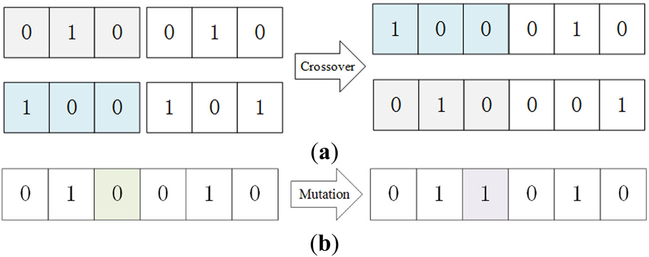
Operations on chromosomes: (a) crossover; (b) mutation.
Step 1: Initialize the parameters and the population. Generate the population (G) with a size of N randomly, and set the crossover probability
Step 2: Calculate the JM of the chromosomes, and select the chromosomes having a higher selection probability pb to generate a new subset of the gene population,
Step 3: Select two parents from
Step 4: Select a locus on a chromosome randomly, and generate a number
Step 5: Evaluate the JM of
3 Experiment and results analysis
In the experiment, the four search algorithms based on their respective swarm intelligence algorithms, as well as the band selection algorithm based on SFFS (BS-SFFS), were tested on both the Indian dataset and the Pavia dataset, respectively. The maximum likelihood (ML) classifier was employed to evaluate the performances of these band selection algorithms, in terms of the JM of band subset, overall classification accuracy (OA), and computational efficiency. For convenience of description, BS-ACA-ML denotes the ML classifier with the band subset provided by BS-ACA, while other notations can be inferred by analogy.
For the four swarm intelligence algorithms, the average Jeffreys–Matusita distances (a-JM) varying with the number of iterations were used to measure the convergence property; at the same time, the classification results in the case of the best JM were presented to demonstrate the discrimination ability of ground features. The average OA as well as the average JM distance of the best band subsets were evaluated on different numbers of bands (5, 10, 15, 20, 25, and 30). The average running time (ART) of algorithms was used to evaluate the computational efficiency. Moreover, the impacts of different population sizes on the best JM, average OA, and computational efficiency were also provided.
These algorithms were encoded with Interact Data Language (IDL) and run under the IDL8.5 compiler on a PC with an Intel(R) Core(TM) CPU i5-4460 processor (3.20 GHz) and 8 GB RAM. To avoid accidental results, all experiments were repeated five times in the same software and hardware environment.
3.1 Parameter setting
Generally, parameters of swarm intelligence algorithm are empirically chosen. In this paper, the parameters of BS-ACA, BS-PSO, and BS-GA were estimated by means of grid searching (see Table 3). The population size of ants, particles, and chromosomes of these algorithms was set to 20. For the BS-CSA, the population size of antibodies is assigned to 10, and the other parameters are listed in Table 3 [34]. The user-specified number of iterations was assigned to 500 for all of the algorithms.
Parameter values for each feature selection algorithm
| BS-ACA | BS-CSA | BS-PSO | BS-GA | ||||
|---|---|---|---|---|---|---|---|
| Parameter | Value | Parameter | Value | Parameter | Value | Parameter | Value |
| Q | 10 | α | 1 | η1 | 2 | Pc | 0.6 |
| ρ | 0.1 | ε | 0.3 | η2 | 2 | Pm | 0.4 |
| α | 1 | r | 0.8 | ||||
| β | 5 | ||||||
3.2 Experiment 1: Indian dataset
3.2.1 Convergence of algorithms
In order to investigate the convergences of these algorithms, band subsets with size of 30 were selected from Indian dataset. Each experiment was repeated five times. The variation in average JM distances with iterations is shown in Figure 6(a). From the figure, it can be seen that BS-ACA and BS-GA were premature and plunged into local optima within 20 and 60 iterations, respectively. BS-CSA could not evolve continuously and took a long time to jump out of the local optima. BS-PSO had been optimizing constantly before converging at the 361st generation. The mean values of the best JM over the five repeated experiments for BS-ACA, BS-CSA, BS-PSO, and BS-GA were 1.48, 1.57, 1.61, and 1.58, respectively. The best JM derived from BS-SFFS was 1.62, approximating to that from BS-PSO, and higher than those of other swarm-intelligence based algorithms.
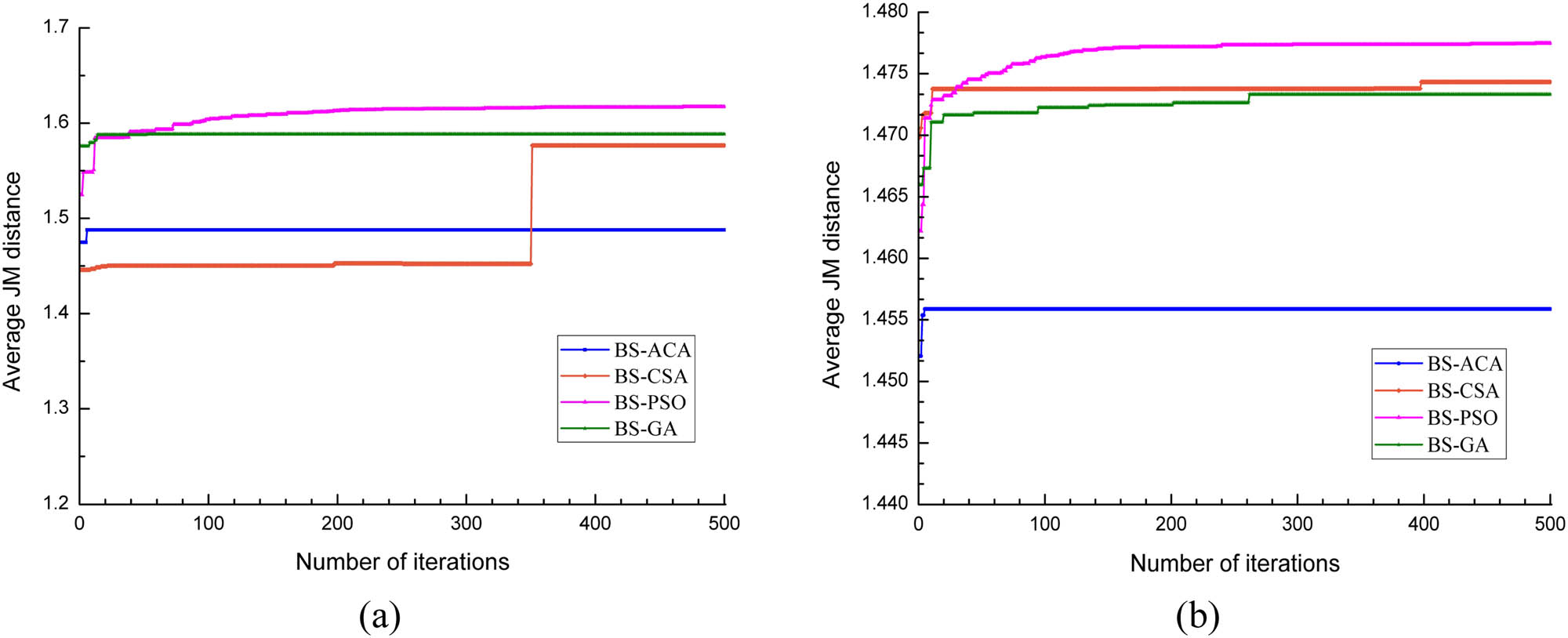
Average JM distance as a function of the number of iterations when the number of selected bands was 30: (a) tested on Indian dataset; (b) tested on Pavia dataset.
3.2.2 Discrimination ability of selected band subsets
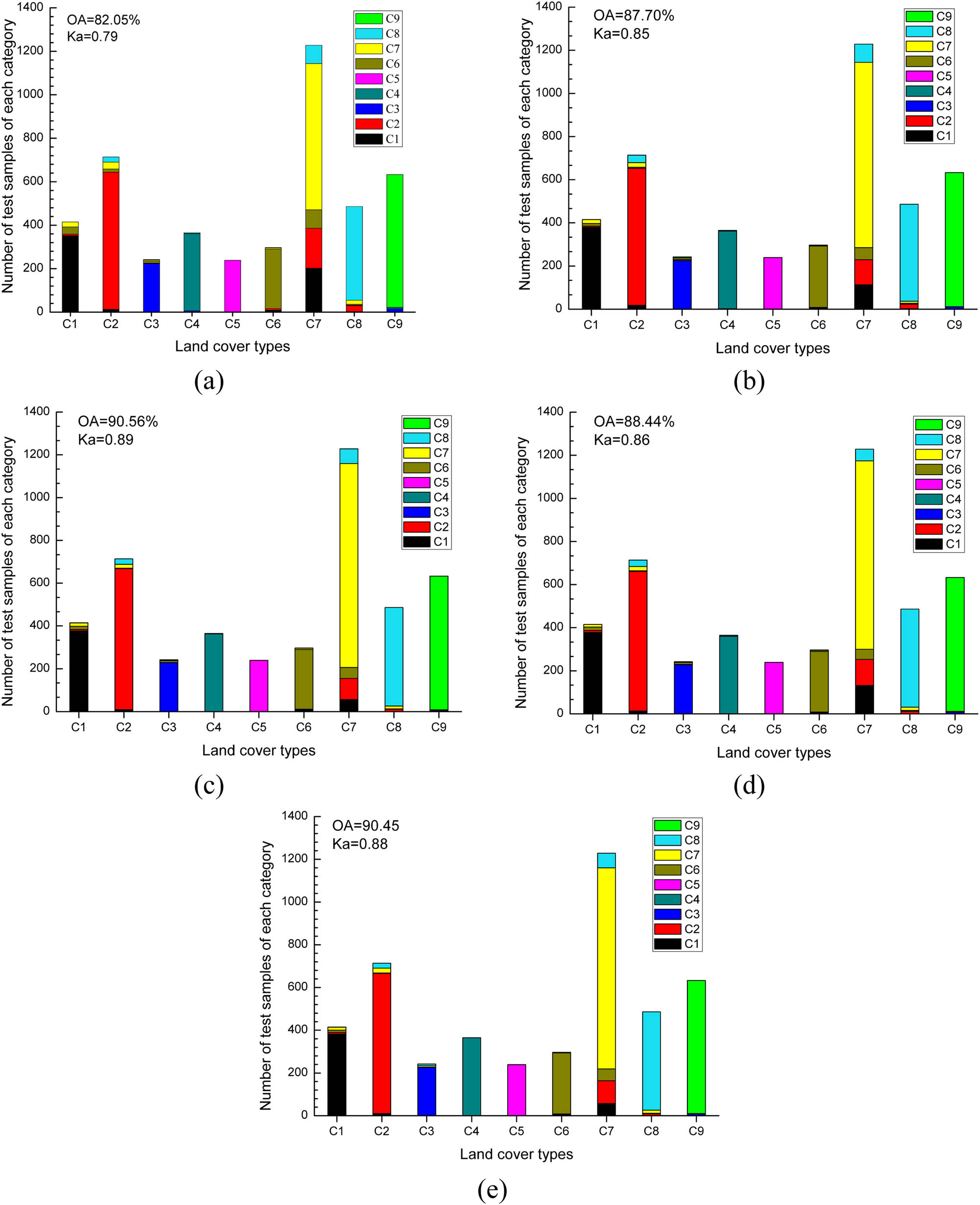
The average OAs of the five search algorithms, by the selected band subsets with size of 30, were 82.05%, 87.66%, 90.15%, 88.44%, and 90.45%, respectively. The best classification results of the algorithms in the five repeated experiments are shown in Figure 7(a–e), respectively, with the corresponding confusion matrices illustrated in Figure 8(a–e). Class-level classifications are also presented by Figures 7 and 8. For the most confusing soybean-mintill that was often misidentified as Corn-mintill and Corn-notill, BS-PSO and BS-SFFS were still superior to BS-ACA, BS-CSA, and BS-GA.

Classification result of the band subsets with the size of 30: (a) BS-ACA; (b) BS-CSA; (c) BS-PSO; (d) BS-GA; (e) BS-SFFS.
Confusion matrix of the classification results of band subsets that were selected by different band selection algorithms: (a) BS-ACA; (b) BS-CSA; (c) BS-PSO; (d) BS-GA; (e) BS-SFFS.
3.2.3 Sizes of band subsets
The performances of the algorithms, resulting from the selected band subsets with different sizes, were compared. As shown in Figure 9, the mean JM and the corresponding average OA were increasing with the size of the band subset for each algorithm. When varying the size of band subsets from 5 to 30, the mean values of the best JM of BS-ACA, BS-CSA, BS-PSO, BS-GA, and BS-SFFS increased from 1.29, 1.28, 1.36, 1.31, and 1.32 to 1.47, 1.57, 1.61, 1.58, and 1.62, respectively. The JM achieved by BS-PSO, approximating to that of BS-SFFS, was higher than those of BS-ACA, BS-CSA, and BS-GA. The corresponding average OAs increased from 65.08%, 64.81%, 72.55%, 69.12%, and 65.19% to 82.05%, 87.66%, 90.15%, 88.44%, and 90.45%. The average OA achieved by BS-PSO-ML was also higher than those of the other swarm-intelligence based algorithms. The average OA of BS-SFFS-ML approximated to that of BS-PSO-ML, except for the size of band subset <10, where a lower OA was obtained in comparison with BS-PSO-ML.
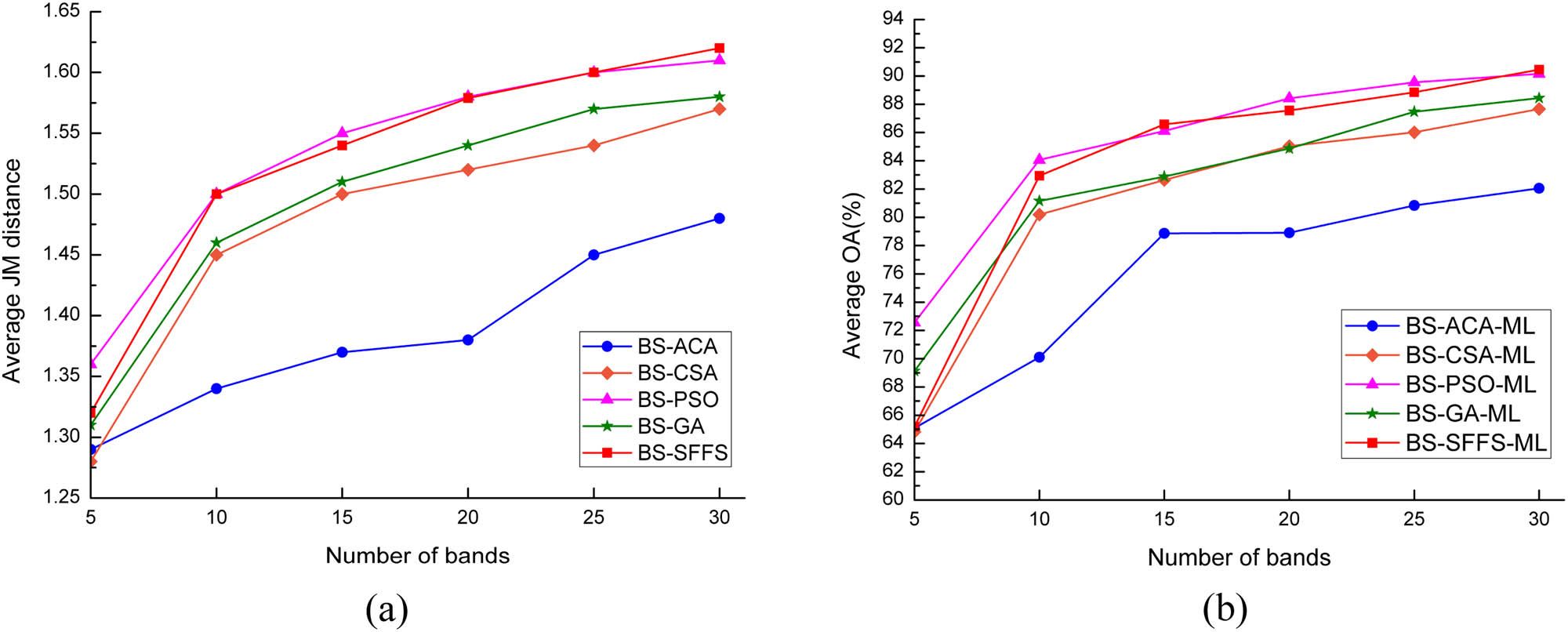
Average JM and average OA as a function of the size of the band subsets derived by the band selection algorithms: (a) the change of average JM distance with the number of bands; (b) the change of average OA with the number of bands.
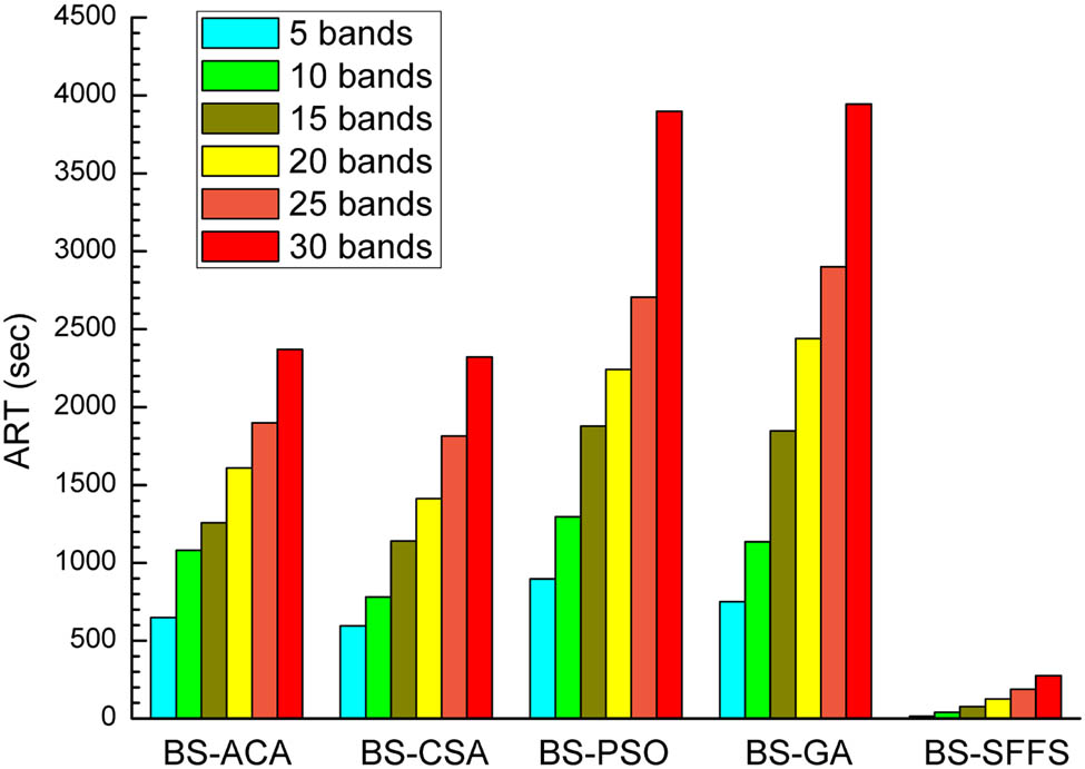
The test results for the ART of the algorithms were obtained and are shown in Figure 10, where 5, 10, 15, 20, 25, and 30 bands were selected from the HSI within 500 iterations. Among the swarm-intelligence based algorithms, the ARTs of BS-CSA and BS-ACA were the smallest, whereas those of BS-PSO and BS-GA were the largest, regardless of the number of selected bands. In terms of the BS-SFFS, the running time was much lower than those of the swarm-intelligence based algorithms, because it did not involve the iterative process.
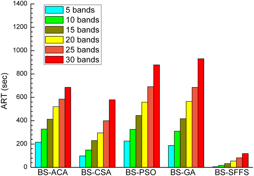
ART as a function of the size of band subsets selected by band selection algorithms.
3.2.4 Impacts of different population sizes
The impacts of different sizes of population on the four swarm-intelligence based algorithms were evaluated. The test results for ART, average JM distance, and average OA are shown in Figure 11. There was no conspicuous impact on the discrimination ability between different land cover types. Instead, the ART was increased markedly. Therefore, it makes no sense to enhance the searching ability of these algorithms by increasing the size of population.
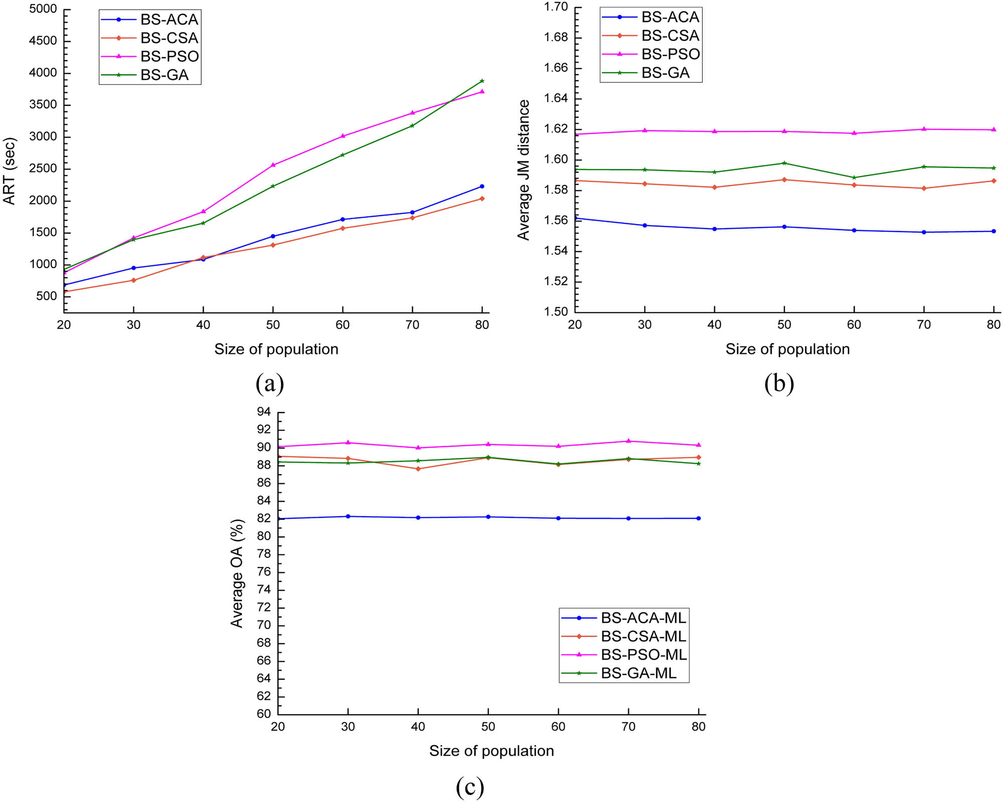
The performance of the swarm intelligence based algorithms with different sizes of population in the Indian dataset experiment: (a) ART; (b) average JM; (c) average OA.
3.3 Experiment 2: Pavia dataset
The band selection algorithms based on swarm intelligence were tested on the Pavia dataset, with the same parameter settings as in experiment 1.
3.3.1 Convergence of algorithms
The convergences of the algorithms relevant to the number of iterations were tested on the Pavia dataset, and the variation in average JM distances with iterations is shown in Figure 6(b). Generally, the convergences of the algorithms appeared in similar patterns to those in experiment 1. The BS-PSO provided the best performance, where the a-JM increased gradually at the beginning and stabilized in the end along with the increase in the number of iterations; whereas the BS-ACA had the worst performance, where it prematurely fell into local optima. The highest a-JM of BS-ACA, BS-CSA, BS-PSO, BS-GA, and BS-SFFS were 1.455, 1.474, 1.477, 1.473, and 1.477, respectively.
3.3.2 Discrimination ability of selected band subsets
The classification images and the corresponding confusion matrices are shown in Figure 12(a–e) and 13(a–e). Band subsets derived from BS-PSO and BS-SFFS had stronger discrimination in ground features than those of the other algorithms. To be specific, BS-PSO-ML and BS-SFFS-ML were inferior to BS-ACA-ML in the matter of the classification of Asphalt and Gravel, but they had better performances for the classification of Meadows and Bare soil.
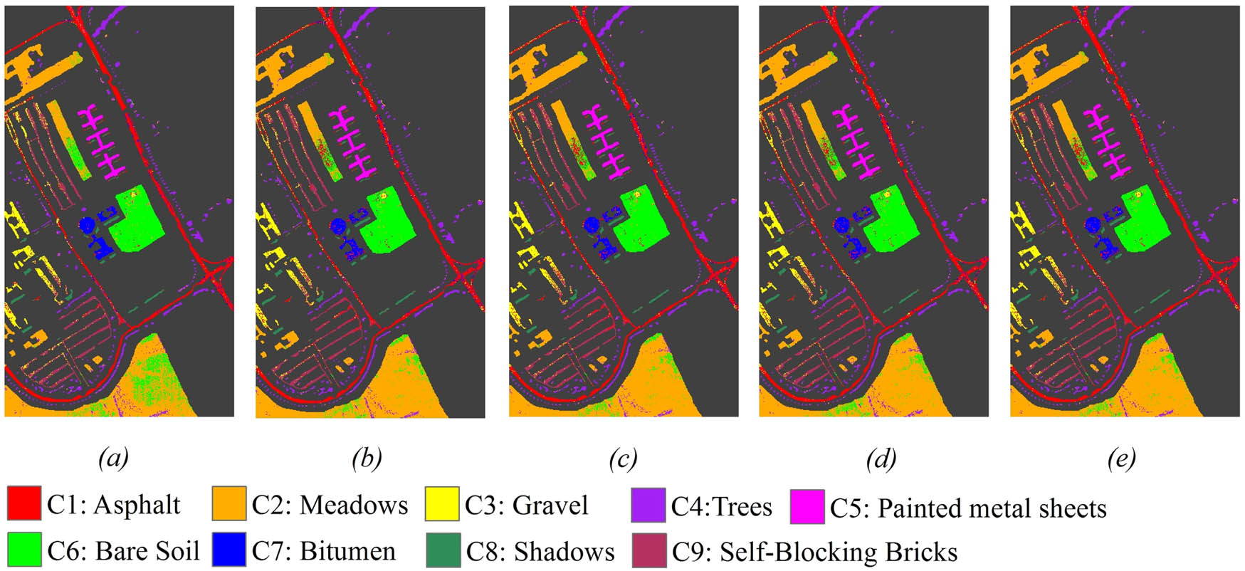
Classification result of the band subsets with the size of 30: (a) BS-ACA; (b) BS-CSA; (c) BS-PSO; (d) BS-GA; (e) BS-SFFS.
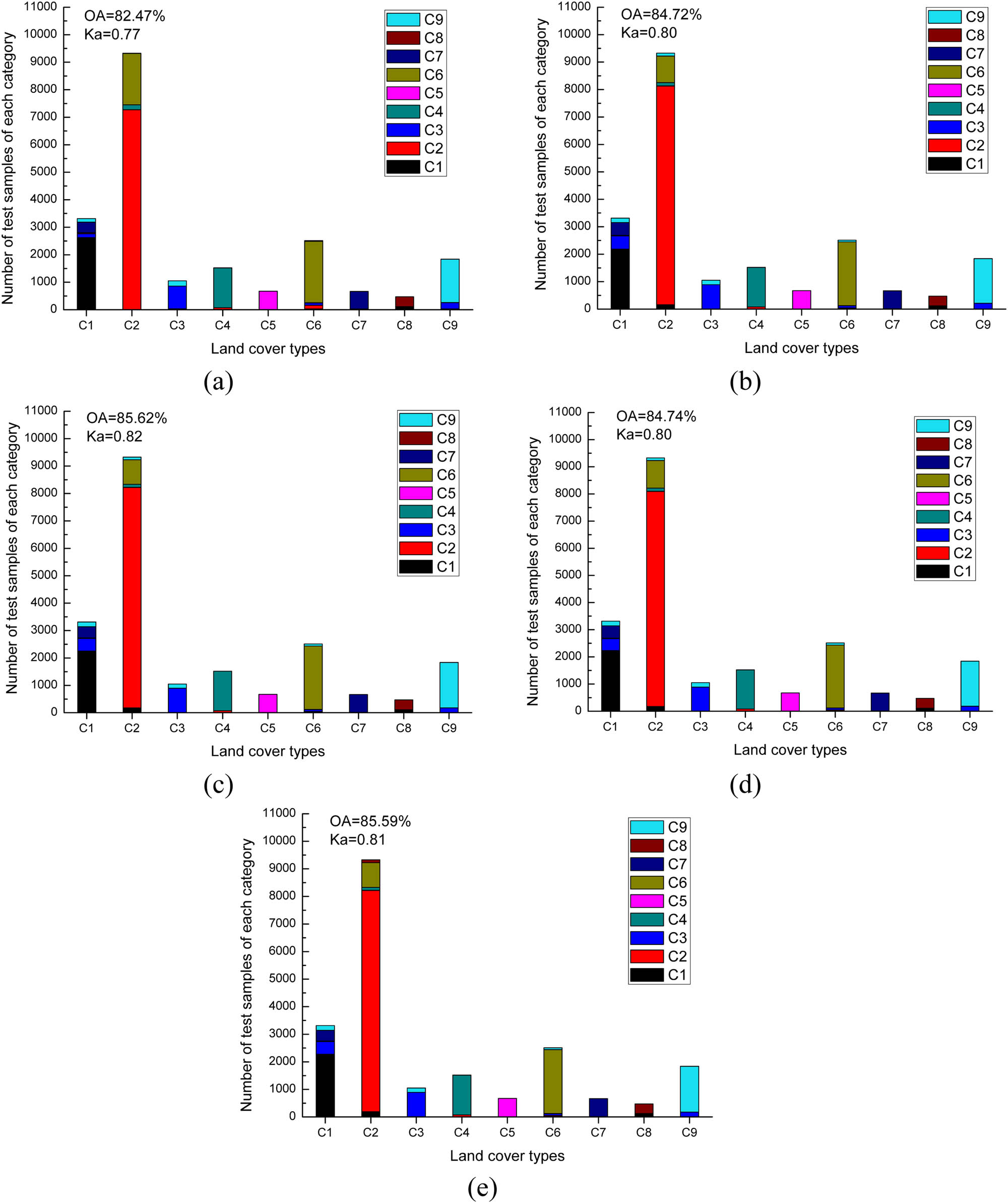
The confusion matrix of classification results of band subset derived from: (a) BS-ACA; (b) BS-CSA; (c) BS-PSO; (d) BS-GA; (e) BS-SFFS.
3.3.3 Sizes of band subset
The responses of the a-JM and average OA to the change in the size of band subset are shown in Figures 14a and b, respectively. The a-JM and the average OA increased with the size of the band subset for each algorithm. In general, the a-JM derived from BS-PSO and BS-SFFS were higher than those of the other three algorithms. The corresponding average OAs achieved by BS-PSO-ML and BS-SFFS-ML were higher than those of BS-ACA-ML, BS-CSA-ML, and BS-GA-ML, whereas the performance of BS-ACA was the worst in terms of a-JM and average OA.
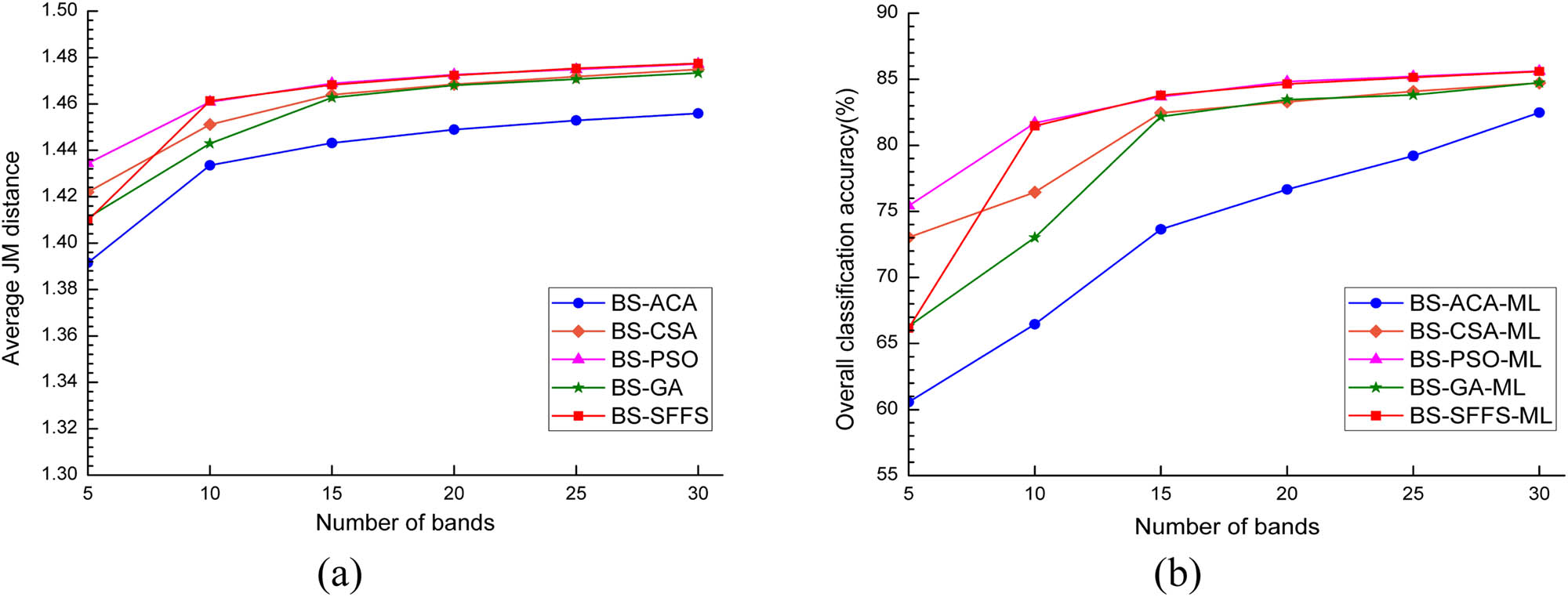
Average JM and average OA as a function of the size of the band subsets derived by the band selection algorithms: (a) the change of average JM distance with the number of bands; (b) the change of average OA with the number of bands.
The corresponding ART of each algorithm for the selection of band subsets with different sizes was obtained and is shown in Figure 15. From the figure, it can be seen that the ART of each algorithm increased with the size of the band subset. The ARTs of BS-PSO and BS-GA were obviously higher than those of BS-ACA and BS-CSA. What’s more, the ART of BS-SFFS was the lowest.
ART as a function of the size of band subsets selected by band selection algorithms.
3.3.4 Impacts of different population sizes
The test results for ART, average JM distance, and average OA are shown in Figure 16. The ARTs of these algorithms have been increased greatly, but the average OAs did not improve markedly. Therefore, it makes no sense to enhance the searching ability of the band selection algorithms by increasing the size of population.

The performance of the swarm intelligence based algorithms with different sizes of population in the Pavia dataset experiment: (a) ART; (b) average JM; (c) average OA.
4 Discussion
A wide range of swarm-intelligence algorithms have been widely used in the feature selection for hyperspectral image classification. Yet, whether the algorithms can constantly choose the optimal features (bands) with consideration of the running time, i.e., the real performance of the algorithms, has not been systematically investigated, which would negatively impact their extensive application. Four typical swarm-intelligence algorithms including the ACA, the CSA, the PSO, and the GA, together with a benchmark called sequent float forward selection (SFFS) – one of the best non-intelligence algorithms, have been tested and compared with two well-known public hyperspectral image datasets (the Indian Pines and the Pavia University).
Generally, compared with the other three swarm-intelligence based algorithms, BS-PSO has stronger optimization capability, which has been demonstrated by the better a-JM, but at a disadvantage in terms of ART.
BS-PSO has the characteristics of evolutionary computation. The “speed-displacement” search strategy, changing particle’s position with iterations by adjusting
BS-ACA is different from the other three algorithms for its searching process that starts from a single ant but does not start with a solution set; it searches for the solution by obtaining the candidate bands one by one with a certain probability. However, when the number of candidate bands is large, the selection probability for the potentially best candidate band is small; thereby, the BS-ACA cannot easily find the better candidate band and will fall into the local optimum. Due to the volatilization of the pheromones that have been laid on the best route, BS-ACA cannot easily jump out of the local optimum. Therefore, BS-ACA has a poor performance in terms of the average JM distance.
The a-JM of BS-CSA and BS-GA are similar and lower than that of BS-PSO. This shows that BS-CSA and BS-GA also fall into local optima. BS-CSA and BS-GA, both use an evolution operator. In BS-CSA, the Ab with higher a-JM has more opportunities to generate offspring and a lower probability of mutating. As a result, the diversity of the population decreases over the generations. BS-GA is similar: in order to maintain a proper convergence speed, the probability of chromosome of being selected is proportional to its a-JM; at the same time, the crossover and mutation operator of BS-GA cannot be activated, unless the crossover probability and mutation probability were met.
The ARTs of these algorithms are different. The running time of algorithm is determined by many factors, such as the computer being used, how and with which programming language the code is implemented [40]. The computational complexity is employed to evaluate the performance of algorithm in terms of running time. In the worst case, the computational time of CSA, required in the optimization problem, is
where s is the number of samples. Thus, the calculation of objective function is time consuming.
ACA and PSO are meta-heuristic algorithms [41]. For BS-ACA, the average JM distance of two different arbitrary bands has been previously calculated in the initialization phase; therefore, much running time can be saved in the iteration process of BS-ACA. Different from BS-ACA, the BS-PSO searches for the optimal band subset by iteratively updating the positions and velocities of the particles. The a-JM of current position and the best position found by each particle must be recalculated after the update operator. Thus, the ART of BS-PSO is greater than that of BS-ACA. BS-CSA and BS-GA are evolutionary algorithms. In most of the cases, the number of cloned Abs (Nc) approximates to N; thus, the calculation of objective function determines the running times of BS-CSA and BS-GA. Although the number of operators in BS-CSA is greater than that of BS-GA, which only has the crossover operator and the mutation operator, the number of chromosomes involved in the crossover and mutation is greater than those of mutated and newly generated Abs. The a-JM of these chromosomes must be recalculated in each generation. However, BS-CSA only needs to calculate the a-JM for the mutated and newly generated Abs. This characteristic saves many computational times for BS-CSA. Therefore, the time consumed by BS-GA is obviously larger than that of BS-CSA. The computational complexity of BS-PSO and BS-GA is the same, and the number of calculation times of the objective function is approximately equal. Therefore, the ARTs of BS-PSO and BS-GA are approximate.
5 Conclusions
In this study, we used four common types of swarm intelligence algorithms and a greedy algorithm to select the optimal band subset from a hyperspectral remote sensing image. The performance was compared from three aspects: a-JM, average OA, and ART.
The experiment results show that the band selection algorithm based on PSO has better performance in terms of average OA, but it needs some improvements to reduce the running time, such as band selection based on parallel PSO [42]. PSO is a potential subset generation procedure for optimal band selection in hyperspectral remote sensing imagery. The band selection algorithm based on the ACA gets into local optima easily. One of the effective methods that can avoid getting into local optima is combined with other algorithms, such as GA, CSA, etc. The performance of the band selection algorithm based on the CSA and that of the band selection algorithm based on the GA were unremarkable, having lower a-JM. A series of evolutionary operators reduced the diversity of the population and led the algorithms to converge to local optima. In brief, PSO has a stronger optimizing capability than the other algorithms, and the optimizing capabilities of the ACA, the CSA, and the GA are weaker than that of SFFS, which is a typical greedy algorithm.
Hence, for the field of band selection in hyperspectral remote sensing imagery, the PSO and the GA have greater room for improvement in achieving an acceptable runtime, and PSO is the best subset generation procedure. These swarm intelligence algorithms can complement each other’s advantages in the structure of a hybrid subset generation procedure having stronger optimizing capabilities.
Acknowledgments
The research was jointly supported by the National Natural Science Foundation of China (Grant Nos.: 41301465, 4197060691), Key Special Project for Introduced Talents Team of Southern Marine Science and Engineering, Guangdong Laboratory (Guangzhou) (Grant No. GML2019ZD0301), the GDAS’ Project of Science and Technology Development (Grant No. 2019GDASYL-0301001), Guangzhou Science and Technology Planning project (Grant No. 201902010033), and the National Key Research and Development Program of China (Grant No. 2016YFB0502300).
References
[1] Huo C, Zhang R, Yin D. Compression technique for compressed sensing hyperspectral images. Int J Remote Sens. 2012;33(5):1586–604. 10.1080/01431161.2011.587843.Suche in Google Scholar
[2] Hughes G. On the mean accuracy of statistical pattern recognizers. IEEE Trans Inform Theory. 1968;14(1):55–63. 10.1109/TIT.1968.1054102.Suche in Google Scholar
[3] Comon P. Independent component analysis, a new concept. Signal Process. 1994;36(3):287–314. 10.1016/0165-1684(94)90029-9.Suche in Google Scholar
[4] Dalla Mura M, Villa A, Benediktsson JA. Jocelyn Chanussot, Lorenzo Bruzzone, Classification of hyperspectral images by using extended morphological attribute profiles and independent component analysis. IEEE Geosci Remote Sens Lett. 2011;8(3):542–6. 10.1109/LGRS.2010.2091253.Suche in Google Scholar
[5] Ma Y, Li R, Yang G, Sun L, Wang J. A research on the combination strategies of multiple features for hyperspectral remote sensing image classification. J Sens. 2018:7341973.10.1155/2018/7341973Suche in Google Scholar
[6] Du Q. Modified fisher’s linear discriminant analysis for hyperspectral imagery. IEEE Geosci Remote Sens Lett. 2007;4(4):503–7. 10.1109/LGRS.2007.900751.Suche in Google Scholar
[7] Ding X, Li H, Yang J, Dale P, Chen X, Jiang C, et al. An improved ant colony algorithm for optimized band selection of hyperspectral remotely sensed imagery. IEEE Access. 2020;8:25789–99.10.1109/ACCESS.2020.2971327Suche in Google Scholar
[8] Talukder A, Casasent D. General methodology for simultaneous representation and discrimination of multiple object classes. Opt Eng. 1998;37(3):904–13. 10.1117/1.601925.Suche in Google Scholar
[9] Nascimento JMP, Dias JMB. Does independent component analysis play a role in unmixing hyperspectral data. IEEE Trans Geosci Remote Sens. 2005;43(1):175–87. 10.1109/TGRS.2004.839806.Suche in Google Scholar
[10] Martínez AM, Kak AC. PCA versus LDA. IEEE Trans Pattern Anal Mach Intell. 2001;23(2):228–33. 10.1109/34.908974.Suche in Google Scholar
[11] Feng J, Jiao L, Liu F, Sun T, Zhang X. Unsupervised feature selection based on maximum information and minimum redundancy for hyperspectral images. Pattern Recognit. 2016;51:295–309. 10.1016/j.patcog.2015.08.018.Suche in Google Scholar
[12] Feng L, Tan AH, Lim MH, Jiang SW. Band selection for hyperspectral images using probabilistic memetic algorithm. Soft Comput. 2016;20(12):4685–93. 10.1007/s00500-014-1508-1.Suche in Google Scholar
[13] Dash M, Liu H. Feature selection for classification. Intell Data Anal. 1997;1(1–4):131–56. 10.1016/S1088-467X(97)00008-5.Suche in Google Scholar
[14] Pudil P, Novovičová J, Kittler J. Floating search methods in feature selection. Pattern Recognit Lett. 1994;15(11):1119–25. 10.1109/ICPR.1994.576920.Suche in Google Scholar
[15] Yang H, Du Q, Chen G. Particle swarm optimization-based hyperspectral dimensionality reduction for urban land cover classification. IEEE J Select Top Appl Earth Observ Remote Sens. 2012;5(2):544–54. 10.1109/JSTARS.2012.2185822.Suche in Google Scholar
[16] Gomez-Chova L, Calpe J, Camps-Valls G, Martin JD, Soria E, Vila J, et al. Feature selection of hyperspectral data through local correlation and SFFS for crop classification. IGARSS 2003. 2003 IEEE International Geoscience and Remote Sensing Symposium. Proceedings (IEEE Cat. No. 03CH37477). Toulouse, France: IEEE; 2003, July. vol. 1, p. 555–7.10.1109/IGARSS.2003.1293840Suche in Google Scholar
[17] Chang CY, Chang CW, Kathiravan S, Lin C, Chen ST. DAG-SVM based infant cry classification system using sequential forward floating feature selection. Multidimension Syst Signal Process. 2017;28(3):961–76.10.1007/s11045-016-0404-5Suche in Google Scholar
[18] Samadzadegan F, Partovi T. Feature selection based on ant colony algorithm for hyperspectral remote sensing images. Hyperspectral Image and Signal Processing: Evolution in Remote Sensing (WHISPERS), 2010 2nd Workshop on IEEE. Reykjavik, Iceland: IEEE; 2010. p. 1–4.10.1109/WHISPERS.2010.5594966Suche in Google Scholar
[19] Eberhart RC, Shi Y, Kennedy J. Swarm intelligence. San Francisco: Elsevier; 2001.Suche in Google Scholar
[20] Zhuo L, Zheng J, Li X, Wang F, Ai B, Qian J. A genetic algorithm based wrapper feature selection method for classification of hyperspectral images using support vector machine. In: Proc. Geoinformat. Joint Conf. GIS Built Environ. Classif. Remote Sens. Images Int Soc Opt Photonics. Bellingham, USA: SPIE; 2008. p. 71471J.10.1117/12.813256Suche in Google Scholar
[21] Al-Ani A. Feature subset selection using ant colony optimization. Int J Comput Intell. 2005;2(1):53–8.Suche in Google Scholar
[22] Zhu X, Li N, Pan Y. Optimization performance comparison of three different group intelligence algorithms on a SVM for hyperspectral imagery classification. Remote Sens. 2019;11(6):734.10.3390/rs11060734Suche in Google Scholar
[23] Zhou S, Zhang J, Su B. Feature selection and classification based on ant colony algorithm for hyperspectral remote sensing images, Image and Signal Processing, 2009. CISP'09. 2nd International Congress on. IEEE, Tianjin, China. 2009. p. 1–4.10.1109/CISP.2009.5304614Suche in Google Scholar
[24] Zhong Y, Zhang L. A fast clonal selection algorithm for feature selection in hyperspectral imagery. Geo-spatial Inform Sci. 2009;12(3):172–81. 10.1007/s11806-009-0098-z.Suche in Google Scholar
[25] Tu CJ, Chuang LY, Chang JY, Yang CH. Feature selection using PSO-SVM. Int J Comput Sci. 2007;33(1):111–6.Suche in Google Scholar
[26] Wang X, Yang J, Teng X, Xia W, Jensen R. Feature selection based on rough sets and particle swarm optimization. Pattern Recognit Lett. 2007;28(4):459–71. 10.1016/j.patrec.2006.09.003.Suche in Google Scholar
[27] Samadzadegan F, Mahmoudi FT. Optimum band selection in hyperspectral imagery using swarm intelligence optimization algorithms, Image Information Processing (ICIIP). 2011 International Conference on. IEEE, Shimla, Himachal Pradesh, India. 2011. p. 1–6.Suche in Google Scholar
[28] Su H, Du Q, Chen G, Du P. Optimized hyperspectral band selection using particle swarm optimization. IEEE J Select Top Appl Earth Observ Remote Sens. 2014;7(6):2659–70. 10.1109/JSTARS.2014.2312539.Suche in Google Scholar
[29] Dorigo M, Di Caro G, Ant colony optimization: a new meta-heuristic, Evolutionary Computation, 1999. CEC 99. Proceedings of the 1999 Congress on. IEEE, Washington, DC, USA, 2, p. 1470–1477.Suche in Google Scholar
[30] Dorigo M, Birattari M, Stutzle T. Ant colony optimization. IEEE Comput Intell Mag. 2006;1(4):28–39. 10.1007/978-0-387-30164-8_22.Suche in Google Scholar
[31] Dréo J, Siarry P. A new ant colony algorithm using the heterarchical concept aimed at optimization of multiminima continuous functions. In: International Workshop on Ant Algorithms. Berlin, Heidelberg: Springer; 2002. p. 216–21. 10.1007/3-540-45724-0_18.Suche in Google Scholar
[32] Dorigo M. Optimization, Learning and Natural Algorithms (in Italian), PhD thesis, Dipartimento di Elettronica, Politecnico di Milano, Italy, 1992.Suche in Google Scholar
[33] Bean WB. The clonal selection theory of acquired immunity. AMA Arch Intern Med. 1960;105(6):973–4. 10.1097/00000441-196104000-00027.Suche in Google Scholar
[34] Zhang L, Zhong Y, Huang B, Gong J, Li P. Dimensionality reduction based on clonal selection for hyperspectral imagery. IEEE Trans Geosci Remote Sens. 2007;45(12):4172–86. 10.1109/TGRS.2007.905311.Suche in Google Scholar
[35] Kennedy J, Eberhart RC. Particle swarm optimization. In: Proceedings of the 1995 IEEE International Conference on Neural Networks. vol. 4, Piscataway, NJ: IEEE Press; 1995. p. 1942–8.10.1109/ICNN.1995.488968Suche in Google Scholar
[36] Potts JC, Giddens TD, Yadav SB. The development and evaluation of an improved genetic algorithm based on migration and artificial selection. IEEE Trans Syst Man Cybernet. 1994;24(1):73–86. 10.1109/21.259687.Suche in Google Scholar
[37] Alba E, Troya JM. A survey of parallel distributed genetic algorithms. Complexity. 1999;4(4):31–52. 10.1002/(SICI)1099-0526(199903/04)4:43.0.CO;2-4.Suche in Google Scholar
[38] Lokman G, Baba AF, Topuz V. A trajectory tracking FLC tuned with PSO for TRIGA Mark-II nuclear research reactor. International Conference on Knowledge-Based and Intelligent Information and Engineering Systems. Berlin, Heidelberg: Springer; 2011. p. 90–9.10.1007/978-3-642-23851-2_10Suche in Google Scholar
[39] Li HP, Zhang SQ, Zhang C, Li P, Cropp R. A novel unsupervised Levy flight particle swarm optimization (ULPSO) method for multispectral remote-sensing image classification. Int J Remote Sens. 2017;38(23):6970–92. 10.1080/01431161.2017.1368102.Suche in Google Scholar
[40] De Castro LN, Von Zuben FJ. Learning and optimization using the clonal selection principle. IEEE Trans Evolution Comput. 2002;6(3):239–51. 10.1109/tevc.2002.1011539.Suche in Google Scholar
[41] Oliveto PS, He J, Yao X. Time complexity of evolutionary algorithms for combinatorial optimization: a decade of results. Int J Automat Comput. 2007;4(3):281–93. 10.1007/s11633-007-0281-3.Suche in Google Scholar
[42] Chang YL, Fang JP, Benediktsson JA, Lena C, Hsuan R, Kun-Shan C. Band selection for hyperspectral images based on parallel particle swarm optimization schemes. In: Geoscience and Remote Sensing Symposium, 2009 IEEE International, IGARSS 2009. IEEE, Cape Town, South Africa. vol. 5, New York, USA: IEEE; 2009. p. V-84–7.10.1109/IGARSS.2009.5417728Suche in Google Scholar
© 2020 Ding Xiaohui et al., published by De Gruyter
This work is licensed under the Creative Commons Attribution 4.0 International License.
Artikel in diesem Heft
- Regular Articles
- The simulation approach to the interpretation of archival aerial photographs
- The application of137Cs and210Pbexmethods in soil erosion research of Titel loess plateau, Vojvodina, Northern Serbia
- Provenance and tectonic significance of the Zhongwunongshan Group from the Zhongwunongshan Structural Belt in China: insights from zircon geochronology
- Analysis, Assessment and Early Warning of Mudflow Disasters along the Shigatse Section of the China–Nepal Highway
- Sedimentary succession and recognition marks of lacustrine gravel beach-bars, a case study from the Qinghai Lake, China
- Predicting small water courses’ physico-chemical status from watershed characteristics with two multivariate statistical methods
- An Overview of the Carbonatites from the Indian Subcontinent
- A new statistical approach to the geochemical systematics of Italian alkaline igneous rocks
- The significance of karst areas in European national parks and geoparks
- Geochronology, trace elements and Hf isotopic geochemistry of zircons from Swat orthogneisses, Northern Pakistan
- Regional-scale drought monitor using synthesized index based on remote sensing in northeast China
- Application of combined electrical resistivity tomography and seismic reflection method to explore hidden active faults in Pingwu, Sichuan, China
- Impact of interpolation techniques on the accuracy of large-scale digital elevation model
- Natural and human-induced factors controlling the phreatic groundwater geochemistry of the Longgang River basin, South China
- Land use/land cover assessment as related to soil and irrigation water salinity over an oasis in arid environment
- Effect of tillage, slope, and rainfall on soil surface microtopography quantified by geostatistical and fractal indices during sheet erosion
- Validation of the number of tie vectors in post-processing using the method of frequency in a centric cube
- An integrated petrophysical-based wedge modeling and thin bed AVO analysis for improved reservoir characterization of Zhujiang Formation, Huizhou sub-basin, China: A case study
- A grain size auto-classification of Baikouquan Formation, Mahu Depression, Junggar Basin, China
- Dynamics of mid-channel bars in the Middle Vistula River in response to ferry crossing abutment construction
- Estimation of permeability and saturation based on imaginary component of complex resistivity spectra: A laboratory study
- Distribution characteristics of typical geological relics in the Western Sichuan Plateau
- Inconsistency distribution patterns of different remote sensing land-cover data from the perspective of ecological zoning
- A new methodological approach (QEMSCAN®) in the mineralogical study of Polish loess: Guidelines for further research
- Displacement and deformation study of engineering structures with the use of modern laser technologies
- Virtual resolution enhancement: A new enhancement tool for seismic data
- Aeromagnetic mapping of fault architecture along Lagos–Ore axis, southwestern Nigeria
- Deformation and failure mechanism of full seam chamber with extra-large section and its control technology
- Plastic failure zone characteristics and stability control technology of roadway in the fault area under non-uniformly high geostress: A case study from Yuandian Coal Mine in Northern Anhui Province, China
- Comparison of swarm intelligence algorithms for optimized band selection of hyperspectral remote sensing image
- Soil carbon stock and nutrient characteristics of Senna siamea grove in the semi-deciduous forest zone of Ghana
- Carbonatites from the Southern Brazilian platform: I
- Seismicity, focal mechanism, and stress tensor analysis of the Simav region, western Turkey
- Application of simulated annealing algorithm for 3D coordinate transformation problem solution
- Application of the terrestrial laser scanner in the monitoring of earth structures
- The Cretaceous igneous rocks in southeastern Guangxi and their implication for tectonic environment in southwestern South China Block
- Pore-scale gas–water flow in rock: Visualization experiment and simulation
- Assessment of surface parameters of VDW foundation piles using geodetic measurement techniques
- Spatial distribution and risk assessment of toxic metals in agricultural soils from endemic nasopharyngeal carcinoma region in South China
- An ABC-optimized fuzzy ELECTRE approach for assessing petroleum potential at the petroleum system level
- Microscopic mechanism of sandstone hydration in Yungang Grottoes, China
- Importance of traditional landscapes in Slovenia for conservation of endangered butterfly
- Landscape pattern and economic factors’ effect on prediction accuracy of cellular automata-Markov chain model on county scale
- The influence of river training on the location of erosion and accumulation zones (Kłodzko County, South West Poland)
- Multi-temporal survey of diaphragm wall with terrestrial laser scanning method
- Functionality and reliability of horizontal control net (Poland)
- Strata behavior and control strategy of backfilling collaborate with caving fully-mechanized mining
- The use of classical methods and neural networks in deformation studies of hydrotechnical objects
- Ice-crevasse sedimentation in the eastern part of the Głubczyce Plateau (S Poland) during the final stage of the Drenthian Glaciation
- Structure of end moraines and dynamics of the recession phase of the Warta Stadial ice sheet, Kłodawa Upland, Central Poland
- Mineralogy, mineral chemistry and thermobarometry of post-mineralization dykes of the Sungun Cu–Mo porphyry deposit (Northwest Iran)
- Main problems of the research on the Palaeolithic of Halych-Dnister region (Ukraine)
- Application of isometric transformation and robust estimation to compare the measurement results of steel pipe spools
- Hybrid machine learning hydrological model for flood forecast purpose
- Rainfall thresholds of shallow landslides in Wuyuan County of Jiangxi Province, China
- Dynamic simulation for the process of mining subsidence based on cellular automata model
- Developing large-scale international ecological networks based on least-cost path analysis – a case study of Altai mountains
- Seismic characteristics of polygonal fault systems in the Great South Basin, New Zealand
- New approach of clustering of late Pleni-Weichselian loess deposits (L1LL1) in Poland
- Implementation of virtual reference points in registering scanning images of tall structures
- Constraints of nonseismic geophysical data on the deep geological structure of the Benxi iron-ore district, Liaoning, China
- Mechanical analysis of basic roof fracture mechanism and feature in coal mining with partial gangue backfilling
- The violent ground motion before the Jiuzhaigou earthquake Ms7.0
- Landslide site delineation from geometric signatures derived with the Hilbert–Huang transform for cases in Southern Taiwan
- Hydrological process simulation in Manas River Basin using CMADS
- LA-ICP-MS U–Pb ages of detrital zircons from Middle Jurassic sedimentary rocks in southwestern Fujian: Sedimentary provenance and its geological significance
- Analysis of pore throat characteristics of tight sandstone reservoirs
- Effects of igneous intrusions on source rock in the early diagenetic stage: A case study on Beipiao Formation in Jinyang Basin, Northeast China
- Applying floodplain geomorphology to flood management (The Lower Vistula River upstream from Plock, Poland)
- Effect of photogrammetric RPAS flight parameters on plani-altimetric accuracy of DTM
- Morphodynamic conditions of heavy metal concentration in deposits of the Vistula River valley near Kępa Gostecka (central Poland)
- Accuracy and functional assessment of an original low-cost fibre-based inclinometer designed for structural monitoring
- The impacts of diagenetic facies on reservoir quality in tight sandstones
- Application of electrical resistivity imaging to detection of hidden geological structures in a single roadway
- Comparison between electrical resistivity tomography and tunnel seismic prediction 303 methods for detecting the water zone ahead of the tunnel face: A case study
- The genesis model of carbonate cementation in the tight oil reservoir: A case of Chang 6 oil layers of the Upper Triassic Yanchang Formation in the western Jiyuan area, Ordos Basin, China
- Disintegration characteristics in granite residual soil and their relationship with the collapsing gully in South China
- Analysis of surface deformation and driving forces in Lanzhou
- Geochemical characteristics of produced water from coalbed methane wells and its influence on productivity in Laochang Coalfield, China
- A combination of genetic inversion and seismic frequency attributes to delineate reservoir targets in offshore northern Orange Basin, South Africa
- Explore the application of high-resolution nighttime light remote sensing images in nighttime marine ship detection: A case study of LJ1-01 data
- DTM-based analysis of the spatial distribution of topolineaments
- Spatiotemporal variation and climatic response of water level of major lakes in China, Mongolia, and Russia
- The Cretaceous stratigraphy, Songliao Basin, Northeast China: Constrains from drillings and geophysics
- Canal of St. Bartholomew in Seča/Sezza: Social construction of the seascape
- A modelling resin material and its application in rock-failure study: Samples with two 3D internal fracture surfaces
- Utilization of marble piece wastes as base materials
- Slope stability evaluation using backpropagation neural networks and multivariate adaptive regression splines
- Rigidity of “Warsaw clay” from the Poznań Formation determined by in situ tests
- Numerical simulation for the effects of waves and grain size on deltaic processes and morphologies
- Impact of tourism activities on water pollution in the West Lake Basin (Hangzhou, China)
- Fracture characteristics from outcrops and its meaning to gas accumulation in the Jiyuan Basin, Henan Province, China
- Impact evaluation and driving type identification of human factors on rural human settlement environment: Taking Gansu Province, China as an example
- Identification of the spatial distributions, pollution levels, sources, and health risk of heavy metals in surface dusts from Korla, NW China
- Petrography and geochemistry of clastic sedimentary rocks as evidence for the provenance of the Jurassic stratum in the Daqingshan area
- Super-resolution reconstruction of a digital elevation model based on a deep residual network
- Seismic prediction of lithofacies heterogeneity in paleogene hetaoyuan shale play, Biyang depression, China
- Cultural landscape of the Gorica Hills in the nineteenth century: Franciscean land cadastre reports as the source for clarification of the classification of cultivable land types
- Analysis and prediction of LUCC change in Huang-Huai-Hai river basin
- Hydrochemical differences between river water and groundwater in Suzhou, Northern Anhui Province, China
- The relationship between heat flow and seismicity in global tectonically active zones
- Modeling of Landslide susceptibility in a part of Abay Basin, northwestern Ethiopia
- M-GAM method in function of tourism potential assessment: Case study of the Sokobanja basin in eastern Serbia
- Dehydration and stabilization of unconsolidated laminated lake sediments using gypsum for the preparation of thin sections
- Agriculture and land use in the North of Russia: Case study of Karelia and Yakutia
- Textural characteristics, mode of transportation and depositional environment of the Cretaceous sandstone in the Bredasdorp Basin, off the south coast of South Africa: Evidence from grain size analysis
- One-dimensional constrained inversion study of TEM and application in coal goafs’ detection
- The spatial distribution of retail outlets in Urumqi: The application of points of interest
- Aptian–Albian deposits of the Ait Ourir basin (High Atlas, Morocco): New additional data on their paleoenvironment, sedimentology, and palaeogeography
- Traditional agricultural landscapes in Uskopaljska valley (Bosnia and Herzegovina)
- A detection method for reservoir waterbodies vector data based on EGADS
- Modelling and mapping of the COVID-19 trajectory and pandemic paths at global scale: A geographer’s perspective
- Effect of organic maturity on shale gas genesis and pores development: A case study on marine shale in the upper Yangtze region, South China
- Gravel roundness quantitative analysis for sedimentary microfacies of fan delta deposition, Baikouquan Formation, Mahu Depression, Northwestern China
- Features of terraces and the incision rate along the lower reaches of the Yarlung Zangbo River east of Namche Barwa: Constraints on tectonic uplift
- Application of laser scanning technology for structure gauge measurement
- Calibration of the depth invariant algorithm to monitor the tidal action of Rabigh City at the Red Sea Coast, Saudi Arabia
- Evolution of the Bystrzyca River valley during Middle Pleistocene Interglacial (Sudetic Foreland, south-western Poland)
- A 3D numerical analysis of the compaction effects on the behavior of panel-type MSE walls
- Landscape dynamics at borderlands: analysing land use changes from Southern Slovenia
- Effects of oil viscosity on waterflooding: A case study of high water-cut sandstone oilfield in Kazakhstan
- Special Issue: Alkaline-Carbonatitic magmatism
- Carbonatites from the southern Brazilian Platform: A review. II: Isotopic evidences
- Review Article
- Technology and innovation: Changing concept of rural tourism – A systematic review