Spatial structure-preserving and conflict-avoiding methods for point settlement selection

2.1 Problems

The density index is one of the most effective means to reduce spatial conflicts in point group map generalization. Existing studies mostly use the area of the Voronoi diagram to measure the density of points to determine whether to select. However, if only the area of the Voronoi diagram is used, the spatial conflicts cannot be effectively avoided. For example, in Figure 1, the Voronoi diagrams of A and B are much larger than those of C and D. If only determined by the Voronoi diagram, C or D will be deleted first. But the distance between points A and B is less than the distance between points C and D. From the perspective of spatial conflict, it is more appropriate to delete either A or B first. Therefore, the area of the Voronoi diagram cannot be simply used to avoid spatial conflicts. Intuitively speaking, the distance between adjacent points is more suitable.

Figure 1

Voronoi diagram and spatial conflict.

2.2 An improved method of avoiding spatial conflicts

In order to more effectively avoid spatial conflict in the selection results, this article considers the conflict distance as a constraint condition. In our improvement, if the shortest distance between the two objects is less than a threshold, d _Th, it is determined that the two are spatial conflicts. d _Th can be determined according to the minimum visible distance on the map (noted as d _v), generally 0.2 or 0.3 mm, or be manually set by the user. Let M be the denominator of the target map scale, then d _Th can be calculated as

Assume that the neighbors of settlement i are N = {N _k }. The shortest distance between i and its neighbors is noted as

where Len() represents the length function.

The neighbor with the shortest distance from i is noted as p, that is, mlen _i = Len(i, p). In this article, if mlen _i ≤ d _Th, then (i, p) is regarded as spatial conflicted. If one is selected, then the other should be deleted. The principle is to delete the settlement with the smallest neighboring shortest distance. That is,

The aforementioned principle gives priority to spatial conflict. Deleting the settlement with the shortest neighboring distance can also avoid subsequent possible conflicts to the greatest extent. If settlement importance is available and is prioritized, the deletion works as follows:

where imp represents the settlement importance.

If mlen _i > d _Th, the selection index should take into account both the Voronoi diagram and the neighboring shortest distance, which is recorded as VAD (Voronoi Area and Distance). For settlement i, its selection index VAD _i is calculated as

where Area _i is the area of the Voronoi diagram corresponding. The larger the Area _i , the larger its spatial influence area; the larger the mlen _i , the greater the absolute distance between settlement i and neighbors, and the smaller the possibility of spatial conflict. Therefore, settlement i is more likely to be selected.

3.1 Problems

According to refs [6,7], when a point is determined to be deleted, its first-order neighboring points are all temporarily solidified and are not allowed to be deleted. This will reduce the candidate number in the subsequent process and may result in the remaining points of high importance being mistakenly deleted. This phenomenon is called “excessive temporary solidification” [15].

In fact, some neighboring points at far distances need not be temporarily solidified. The root cause is the use of Voronoi diagrams to qualitatively measure spatial proximity. This drawback is even much worse in spatial conditions such as clusters and the boundary of groups [16].

On the other hand, the existing distance-based spatial proximity measuring methods lack the ability to continuously divide the spatial competition relationship. The buffer zone can determine the proximity relationship by the intersection (Figure 2a), but it cannot accurately determine the natural spatial competition relationship among objects and their domains of influence, that is, it cannot achieve the continuity and non-overlap division of the entire space. Although existing subdivisions, such as grids and hexagons, can perform continuous spatial division (as in Figure 2b), the division unit is generally global and is fixed. There are at least the following problems.

1. It cannot be guaranteed that each object has a subdivision unit on its own, as in Figure 2b, even if the “window moving” strategy [11] is adopted.

2. The spatial continuous division pays less attention to the natural spatial competition. The subdivision accuracy is still directly related to the grid size and cannot be natural and continuous.

Figure 2

Different spatial divisions. (a) Buffer zone; (b) grid; and (c) DCV.

That is to say, the distance-based methods cannot overcome the shortcomings of the Voronoi diagram. Hence, we improve and design a DCV diagram model.

3.2 DCV diagram

Utilizing Voronoi diagrams to measure the proximity relationship has obvious shortcomings in point settlement selection [17], and the distance method cannot make up for its shortcomings. Basaraner used the intersection of the Voronoi zone and the buffer of buildings in a cluster as a generalization zone in displacement operations [18]. To this end, this article combines both the advantages of spatial division (such as Voronoi) and distance measurement and proposes a novel DCV diagram model, which is used to improve the spatial proximity measurement in settlement selection.

Actually, a good spatial division should satisfy two aspects: (1) determining a division principle and (2) constraining the spatial region by a certain distance measurement. Hence, we use the Voronoi diagram to achieve spatial division and employ the distance to constrain the Voronoi polygon to the specified spatial region. The proposed DCV diagram is the intersection of the original Voronoi and the distance-constrained region (such as a buffer analysis). The method is discussed subsequently in detail.

Take the point in Figure 2c as an example. Its ordinary Voronoi polygon is the polygon composed of six edges, A, B, C, D, E, and F. If we want to constrain the Voronoi polygon within a certain distance, we calculate its intersection with the distance-constrained buffer circle. The resulting shaded part, as in Figure 2c, is the expected DCV result.

Observing the Voronoi polygon and the distance-constrained buffer circle region, we can find that the edges of the Voronoi polygon can be divided into three categories.

1. For the edges located inside the distance constraint circle buffer region, such as edge A, they have remained completely in DCV.

2. For the edges that are intersected with the buffer, such as edges B, C, and F, the parts located inside are retained in DCV, and the other parts are replaced by the corresponding part of the buffer.

3. For the edges outside the buffer, such as edges D and E, they are replaced by the corresponding part of the buffer.

The DCV not only achieves the continuous division of space but also realizes the quantitative proximity measure using distance constraints. Hence, the DCV is more scientific and reasonable in measuring neighboring relationships in the challenge cases of clustered settlement groups and their boundaries. Therefore, the DCV contributes to the selection map generalization operation in spatial distribution characteristics preserving.

3.3 Adaptive temporary solidification strategy to preserve spatial structure

The existing literature [6,7] temporarily solidifies all the first-order neighbors, failing to consider the local spatial characteristics. In fact, the local spatial characteristics around each object are usually different due to spatial heterogeneity [16].

In this section, an adaptive temporary solidification strategy is proposed. Aiming to avoid the phenomenon of excessive temporary solidification, the distance threshold is dynamically calculated and adapted to the local spatial characteristics.

For the Delaunay triangulation G of the point settlements, note the nodes as V = {v _i ，0 ≤ i ≤ N _v }, note the edges as E = {e _i , 0 ≤ i ≤ N _e }, and note the length of edge e _i as L _i . Then the length average of E can be calculated as:

The length standard deviation of E is

For node v _i , according to the Voronoi-K nearest neighbor model method in ref. [19], query all its neighboring edges of K-order to form a set NE K ( v i ) = { e i } . And note the number of the set as n = ∣ NE K ( v i ) ∣ , that is, the number of neighboring edges. Thus, the local length average of the K-order local neighborhood of node v _i is calculated as follows:

where L _k is the length of e k ∈ NE K ( v i ) .

Therefore, for the point settlement i, in the temporary solidification stage by DCV, the local threshold r _Th is dynamically calculated as follows:

In formula (9), α is the harmonic coefficient, which is set to 1 by default. The larger the α, the larger the r _Th, and the larger the temporary solidification region. It can be seen that the local threshold r _Th of each settlement i is jointly determined by the global factor and the local K-order neighbors.

Taking the point settlements in Figure 3 as an example, the ordinary Voronoi diagram is shown in Figure 3a. In Figure 3b, the DCV is constrained by the global length mean of the Delaunay triangulation, which is globally calculated and fixed according to ref. [15]. In Figure 3c, the DCV is constrained by r _Th, which is adaptively and dynamically calculated as above. By comparison, it can be found that:

1. For a settlement that is far away, the proximity determined by the ordinary Voronoi diagram is considered to be spatially adjacent. However, it is obviously unreasonable, which is also against the first law of geography. More details are discussed in ref. [17]. Furthermore, the influence of the settlement at the boundary of the group may be erroneously amplified; that is, the boundary effect of the group cannot be handled well.

2. For the DCV diagram, the distance is critical. If it is manually set as a fixed threshold, then it requires prior knowledge, which is generally difficult to obtain. The DCV in Figure 3b considers the global scope, and all the influence domains are the same, which cannot reflect spatial heterogeneity. The adaptive DCV in Figure 3c can reflect both the global and local characteristics of each settlement, which is more advantageous.

Figure 3

Different Voronoi diagram. (a) Ordinary Voronoi diagram, (b) global DCV, and (c) adaptive DCV.

However, for some isolated settlements, their DCVs may be the buffers of the same size. Their selection criteria are not distinguishable enough. Hence, in the selection operation, the VAD in Section 2 is used as the selection criterion, and the DCV in Section 3 is used to conduct the temporary solidification.

Since the geometrical type of settlement in this article is the point, the computing complexity of the Voronoi diagram and buffer circle is greater than that of the distance between points. Therefore, a simplified version of DCV is adopted. The basic idea is as follows: if the Voronoi diagrams of two points are adjacent, they are treated as candidate neighbors; furthermore, if the distance between them is less than r _Th, they are determined as true neighbors, and the temporary solidification will work only in this situation.

At this time, a temporary solidification strategy works as follows: for the settlement i that is marked as deletion, if the distance between i and its true neighbor j is less than r _Th, then settlement j is temporarily solidified and cannot be deleted in this iteration.

5.1 Spatial conflict-avoiding experiments

Two experiments were conducted to verify the effectiveness. In Experiment 1, although spatial conflicts occur, the selection number can still meet the quantity determined by the Radical Law after the spatial conflicts are removed. In Experiment 2, because of the spatial conflict, the selection number does not meet the selection quantity determined by the Radical Law. The purpose of the latter is to confirm that our method gives more attention to guaranteeing the map quality and readability than mechanically maintaining selection quantity. All the results are rendered in quantum geographical information system. The data are from the National Land Survey of Finland Topographic Database, which are freely available at https://www.maanmittauslaitos.fi/en/e-services/open-data-file-download-service.

In the first experiment, point settlements on a scale of 1:250,000 are tested. The dataset contains 421 point settlements, such as both solid and hollow ones in Figure 5a. Limited to page size, they are not displayed at the real map scale. In order to verify the superiority of our method in spatial conflict-avoiding, comparative experiments were conducted with the method in refs [6,7]. The target map scale is 1:500,000. The selection number is about 295, which was calculated according to the Radical Law [20,21]. Assuming that the minimum visible distance on the map is 0.2 mm, the corresponding field distance is 100 m, so the parameter d _Th = 100 m.

Figure 5

Comparison of the spatial conflict-avoiding selection results between (a) the existing research and (b) our method.

Using the method of refs [6,7], the selection result has 295 settlements, as the solid points shown in Figure 5a, where the hollow points represent the unselected ones. It can be seen that some unreasonable phenomena, such as symbol clutter, exist in the selection result, as boxes A and B in Figure 5a.

In our method, the original dataset is first scaled to the target scale to detect spatial conflicts. The conflict results are shown in Figure 6a, where the solid points connected by lines represent the conflicted settlement pairs. Using the method in Section 2 to solve the spatial conflict, 39 settlements are deleted. Using our proposed method, there are also 295 settlements selected, as shown in Figure 5b. Compared with Figure 5a, the spatial conflicts are basically resolved in Figure 5b.

Limited to page size, only the result in box A in Figure 5a is enlarged for further analysis, as shown in Figure 6b–d. Figure 6b shows the spatial conflicts, where the settlement pairs connected by lines indicate that the distance is less than 100 m. Figure 6c is the selection result of the existing method, and it can be seen that some settlements with spatial conflicts are unreasonably selected, as the details shown in boxes A and B in Figure 6c. Figure 6d shows the selection results by our method, where the spatial conflicts are basically removed. It should be noted that Figure 6c and d is the collaborative generalization results of spatial conflict-avoiding, structural, and geometrical selection algorithms, instead of only considering the spatial conflict-avoiding. Therefore, the conflicted settlement pairs are both deleted in some cases.

Figure 6

Spatial conflicts and the selection results, including (a) the spatial conflicts, (b) the enlarged view, (c) the selection result of the existing research, and (d) the selection result of our method.

In the second experiment, the map scale is 1:500,000. The dataset contains 238 point settlements. The target map scale is 1:1,000,000. The selection number is about 167, according to the Radical Law. Assuming that the minimum visible distance on the map is 0.2 mm, the corresponding field distance is 200 m, so the parameter d _Th = 200 m.

About 168 settlements are selected by the method of refs [6,7], as shown by the solid points in Figure 7a. It is obvious that some unreasonable phenomena, such as symbol clutter, exist, as shown by the boxes in Figure 7a. Using our proposed method, 146 settlements are selected, as shown in Figure 7b. It is obvious that the unreasonable symbol clutter in Figure 7a is removed in Figure 7b. Compared with Figure 7a, extra 22 settlements are deleted due to the spatial conflict, which means we give more priority to quality rather than quantity.

Figure 7

Comparison of selection results between (a) the existing research and (b) our method, where (c–f) are the enlarged views.

Due to page limitations, only the results in boxes A and B in Figure 7a are enlarged for comparative analysis, as shown in Figure 7c–f. It can be seen from the enlarged views that the spatial conflicts in the existing method are all resolved.

5.2 Excessive temporary solidification-avoiding experiments

In order to verify the effectiveness of the DCV in avoiding excessive temporary solidification, experimental point settlements at a scale of 1:25,000 are tested. The dataset contains 347 point settlements with heterogenetic spatial density and obvious clusters. Hence, the excessive temporary solidification avoiding strategy using DCV is employed. The target map scale is 1:50,000. The selection number is about 243, calculated according to the Radical Law. Using the method of refs [6,7], the selection result has 243 settlements as shown in Figure 8a. Figure 8b shows the result of our proposed method, which has 242 settlements.

Figure 8

Comparison of the excessive temporary solidification selection results between (a) the existing research and (b) our adaptive DCV method.

Since the algorithm is an iterative process, in order to better observe the effectiveness of avoiding excessive temporary solidification avoiding method, the first iteration of both methods is selected and shown in Figure 9a and b, respectively. In both methods, 92 point settlements are deleted. In Figure 9a, the settlement pairs connected by the same arrow are regarded as neighbors based on the ordinary Voronoi diagram. According to refs [6,7], they cannot be simultaneously deleted. However, from the perspective of human spatial cognition, these marked pairs obviously belong to different groups, respectively, and therefore should not be temporarily solidified by each other. That is to say, the spatial proximity relationship obtained by the ordinary Voronoi diagram brings unreasonable, excessive temporary solidification. Compared with Figure 9a, the settlement pairs connected by the same arrow in Figure 9b are not regarded as neighbors by DCV because they do not share common edges, so they will not affect each other. This confirms the fact that the adaptive DCV pays more attention to the local spatial characteristics and can avoid unreasonable, excessive temporary solidification phenomena.

Figure 9

The first iteration selection results of (a) ordinary Voronoi diagram and (b) adaptive DCV.

5.3 Experiment of the Overall Selection Methodology

Next, the experiment is carried out on the whole scope of Finland to verify the overall proposed selection methodology. The source map scale is 1:2,000,000, and the target map scales are 1:4,500,000 and 1:8,000,000. The original data contain 454 point settlements. According to the classic Radical Law, the corresponding selection numbers of the two target scales are calculated to be about 299 and 226, respectively. The d _Th of the two target scales are 900 and 1,600 m, respectively. According to the algorithm in this article, the corresponding results are shown in Figure 10. Limited to page space, only part of the map result is displayed. The analysis is as follows.

1. The shortest distances between points on the two target maps are 3812.10 and 7728.19 m, respectively, which are both greater than the minimum visible distance on the map at the target scales. It proves that the proposed method can effectively solve the spatial conflict.

2. According to the current results, the spatial structure characteristics such as spatial density have been basically maintained. The settlements in dense regions of the source map have not been continuously deleted. The relative density contrasts between different regions are still well remained. There is no unreasonable phenomenon that spatial density or structure suffers a dramatic sharp change. This also reflects the effectiveness and advantage of this article in maintaining the spatial structure.

3. The present experiment is only to verify the effectiveness of this article in conflict-avoiding and spatial structure-preserving. So the two results only consider the settlements. We display the selection results using OpenStreetMap as the base map for visual evaluation. In practical application, it is necessary to comprehensively consider the mutual influence of other objects, such as road networks, the object grade, map use, different cartographic specifications, and data characteristics. The collaborative map generalization has a very larger research scope and depends highly on many other technologies, which go beyond the focus of this article. So the above figures are not the final results of the published map products. Figure 10 is also not displayed at the real map scale but limited to page space.

4. The selection quantity here is calculated only using the original classic Radical Law. In practical application, it needs to be modified according to the amount of map information load so as to meet the unification of map legibility and map readability and interpretation. Hence, the selection quantity may be more or less.

Figure 10

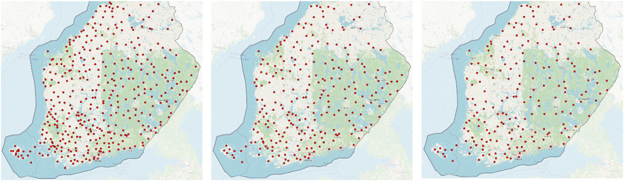
Selection results at different map scales. (a) The source map at the scale of 1:2,000,000, (b) the target map at the scale of 1:4,500,000, and (c) the target map at the scale of 1:8,000,000.

References

[1] Mackaness WA, Ruas A, Sarjakoski LT, editors. Generalisation of geographic information: Cartographic modelling and applications. Amsterdam: Elsevier; 2007.Search in Google Scholar
[2] Wu F, Gong X, Du J. Overview of the research progress in automated map generalization. Acta Geod Cartograp Sin. 2017;46(10):1645–64.Search in Google Scholar
[3] Sen A, Gokgoz T, Sester M. Model generalization of two different drainage patterns by self-organizing maps. Cartograp Geog Inf Sci. 2014;41(2):151–65.10.1080/15230406.2013.877231Search in Google Scholar
[4] Gong X. Research on settlement generalization methods considering spatial pattern and road networks. PhD thesis. Zhengzhou, China: Information Engineering University; 2017.Search in Google Scholar
[5] Gong X, Wu F, Li J, Du J. An extended morphing approach for linear feature displacement. J Geomat Sci Technol. 2018;35(3):291–7.Search in Google Scholar
[6] Yan H, Wang J. A generic algorithm for point cluster generalization based on Voronoi diagrams. J Image Graph. 2005;10(5):633–6.Search in Google Scholar
[7] Ai T, Liu Y. A method of point cluster simplification with spatial distribution properties preserved. Acta Geod Cartograp Sin. 2002;31(2):175–81.Search in Google Scholar
[8] Bereuter P, Weibel R. Real-time generalization of point data in mobile and web mapping using quadtrees. Cartograp Geog Inf Sci. 2013;40(4):1–11.10.1080/15230406.2013.779779Search in Google Scholar
[9] Raposo P, Brewer CA, Stanislawski LV. Label and attribute-based topographic point thinning. 16th ICA Workshop on Generalisation and Multiple Representation, Dresden, Germany; August, 2013. p. 23–4.Search in Google Scholar
[10] Schwartges N, Allerkamp D, Haunert JH, Wolff A. Optimizing active ranges for point selection in dynamic maps. 16th ICA Workshop on Generalisation and Multiple Representation, Dresden, Germany; August, 2013. p. 23–4.Search in Google Scholar
[11] Zhang X, Wang S, Wang Y. Clutter-free visualization of large point symbols at multiple scales by offset quadtrees. Acta Geod Cartograph Sin. 2016;45(8):983–91.Search in Google Scholar
[12] Du J, Wu F, Li J. Line simplification method based on multi-bends groups division. J Comput Des Comput Graph. 2017;29(9):1705–12.10.3724/SP.J.1089.2017.16609Search in Google Scholar
[13] Xing R, Wu F, Li J, Gong X. A fast algorithm of contour generation considering ambiguity. J Comput-Aided Design Comput Graph. 2017;29(9):1705–12.Search in Google Scholar
[14] Gao K, Yang M, Zhang Y. A method of automatic selection of hash-style habitation with spatial distribution characteristics preserved. J Geomat Sci Technol. 2015;32(6):626–30.Search in Google Scholar
[15] Li S, Zhang L, Wen L, Jia S. An improved algorithm of point cluster selection based on Voronoi diagrams and its application in aids to navigation selection. Hydrograph Surv Charting. 2015;35(6):50–4.Search in Google Scholar
[16] Shi Y, Liu Q, Deng M, Lin X. A hybrid spatial clustering method based on graph theory and spatial density. Geomat Inf Sci Wuhan Univ. 2012;37(11):1276–80.Search in Google Scholar
[17] Sang ETK. Voronoi diagrams without bounding boxes. Proceedings of the Joint International Geoinformation Conference 2015, Kuala Lumpur, Malaysia; 2015. II-2/W2:p. 235–9.10.5194/isprsannals-II-2-W2-235-2015Search in Google Scholar
[18] Basaraner M. A zone-based iterative building displacement method through the collective use of Voronoi Tessellation, spatial analysis and multicriteria decision making. Bull Geod Sci. 2011;17(2):161–87.10.1590/S1982-21702011000200001Search in Google Scholar
[19] Gong X. Research on typical map pattern recognition in Urban building groups. Master thesis. Zhengzhou, China: Information Engineering University; 2014.Search in Google Scholar
[20] Gong X, Cui X, Xing R, Liu C. A novel interpolation square root model for multi-scale spatial database. IOP Conf Series Earth and Environ Sci. 2019;310:022042. 10.1088/1755-1315/310/2/022042.Search in Google Scholar
[21] Töpfer F, Pillewizer W. The principles of selection. Cartogr J. 1966;3:10–6.10.1179/caj.1966.3.1.10Search in Google Scholar
© 2022 Gong Xianyong et al., published by De Gruyter
This work is licensed under the Creative Commons Attribution 4.0 International License.
Articles in the same Issue
- Regular Articles
- Study on observation system of seismic forward prospecting in tunnel: A case on tailrace tunnel of Wudongde hydropower station
- The behaviour of stress variation in sandy soil
- Research on the current situation of rural tourism in southern Fujian in China after the COVID-19 epidemic
- Late Triassic–Early Jurassic paleogeomorphic characteristics and hydrocarbon potential of the Ordos Basin, China, a case of study of the Jiyuan area
- Application of X-ray fluorescence mapping in turbiditic sandstones, Huai Bo Khong Formation of Nam Pat Group, Thailand
- Fractal expression of soil particle-size distribution at the basin scale
- Study on the changes in vegetation structural coverage and its response mechanism to hydrology
- Spatial distribution analysis of seismic activity based on GMI, LMI, and LISA in China
- Rock mass structural surface trace extraction based on transfer learning
- Hydrochemical characteristics and D–O–Sr isotopes of groundwater and surface water in the northern Longzi county of southern Tibet (southwestern China)
- Insights into origins of the natural gas in the Lower Paleozoic of Ordos basin, China
- Research on comprehensive benefits and reasonable selection of marine resources development types
- Embedded deformation of the rubble-mound foundation of gravity-type quay walls and influence factors
- Activation of Ad Damm shear zone, western Saudi Arabian margin, and its relation to the Red Sea rift system
- A mathematical conjecture associates Martian TARs with sand ripples
- Study on spatio-temporal characteristics of earthquakes in southwest China based on z-value
- Sedimentary facies characterization of forced regression in the Pearl River Mouth basin
- High-precision remote sensing mapping of aeolian sand landforms based on deep learning algorithms
- Experimental study on reservoir characteristics and oil-bearing properties of Chang 7 lacustrine oil shale in Yan’an area, China
- Estimating the volume of the 1978 Rissa quick clay landslide in Central Norway using historical aerial imagery
- Spatial accessibility between commercial and ecological spaces: A case study in Beijing, China
- Curve number estimation using rainfall and runoff data from five catchments in Sudan
- Urban green service equity in Xiamen based on network analysis and concentration degree of resources
- Spatio-temporal analysis of East Asian seismic zones based on multifractal theory
- Delineation of structural lineaments of Southeast Nigeria using high resolution aeromagnetic data
- 3D marine controlled-source electromagnetic modeling using an edge-based finite element method with a block Krylov iterative solver
- A comprehensive evaluation method for topographic correction model of remote sensing image based on entropy weight method
- Quantitative discrimination of the influences of climate change and human activity on rocky desertification based on a novel feature space model
- Assessment of climatic conditions for tourism in Xinjiang, China
- Attractiveness index of national marine parks: A study on national marine parks in coastal areas of East China Sea
- Effect of brackish water irrigation on the movement of water and salt in salinized soil
- Mapping paddy rice and rice phenology with Sentinel-1 SAR time series using a unified dynamic programming framework
- Analyzing the characteristics of land use distribution in typical village transects at Chinese Loess Plateau based on topographical factors
- Management status and policy direction of submerged marine debris for improvement of port environment in Korea
- Influence of Three Gorges Dam on earthquakes based on GRACE gravity field
- Comparative study of estimating the Curie point depth and heat flow using potential magnetic data
- The spatial prediction and optimization of production-living-ecological space based on Markov–PLUS model: A case study of Yunnan Province
- Major, trace and platinum-group element geochemistry of harzburgites and chromitites from Fuchuan, China, and its geological significance
- Vertical distribution of STN and STP in watershed of loess hilly region
- Hyperspectral denoising based on the principal component low-rank tensor decomposition
- Evaluation of fractures using conventional and FMI logs, and 3D seismic interpretation in continental tight sandstone reservoir
- U–Pb zircon dating of the Paleoproterozoic khondalite series in the northeastern Helanshan region and its geological significance
- Quantitatively determine the dominant driving factors of the spatial-temporal changes of vegetation-impacts of global change and human activity
- Can cultural tourism resources become a development feature helping rural areas to revitalize the local economy under the epidemic? An exploration of the perspective of attractiveness, satisfaction, and willingness by the revisit of Hakka cultural tourism
- A 3D empirical model of standard compaction curve for Thailand shales: Porosity in function of burial depth and geological time
- Attribution identification of terrestrial ecosystem evolution in the Yellow River Basin
- An intelligent approach for reservoir quality evaluation in tight sandstone reservoir using gradient boosting decision tree algorithm
- Detection of sub-surface fractures based on filtering, modeling, and interpreting aeromagnetic data in the Deng Deng – Garga Sarali area, Eastern Cameroon
- Influence of heterogeneity on fluid property variations in carbonate reservoirs with multistage hydrocarbon accumulation: A case study of the Khasib formation, Cretaceous, AB oilfield, southern Iraq
- Designing teaching materials with disaster maps and evaluating its effectiveness for primary students
- Assessment of the bender element sensors to measure seismic wave velocity of soils in the physical model
- Appropriated protection time and region for Qinghai–Tibet Plateau grassland
- Identification of high-temperature targets in remote sensing based on correspondence analysis
- Influence of differential diagenesis on pore evolution of the sandy conglomerate reservoir in different structural units: A case study of the Upper Permian Wutonggou Formation in eastern Junggar Basin, NW China
- Planting in ecologically solidified soil and its use
- National and regional-scale landslide indicators and indexes: Applications in Italy
- Occurrence of yttrium in the Zhijin phosphorus deposit in Guizhou Province, China
- The response of Chudao’s beach to typhoon “Lekima” (No. 1909)
- Soil wind erosion resistance analysis for soft rock and sand compound soil: A case study for the Mu Us Sandy Land, China
- Investigation into the pore structures and CH4 adsorption capacities of clay minerals in coal reservoirs in the Yangquan Mining District, North China
- Overview of eco-environmental impact of Xiaolangdi Water Conservancy Hub on the Yellow River
- Response of extreme precipitation to climatic warming in the Weihe river basin, China and its mechanism
- Analysis of land use change on urban landscape patterns in Northwest China: A case study of Xi’an city
- Optimization of interpolation parameters based on statistical experiment
- Late Cretaceous adakitic intrusive rocks in the Laimailang area, Gangdese batholith: Implications for the Neo-Tethyan Ocean subduction
- Tectonic evolution of the Eocene–Oligocene Lushi Basin in the eastern Qinling belt, Central China: Insights from paleomagnetic constraints
- Geographic and cartographic inconsistency factors among different cropland classification datasets: A field validation case in Cambodia
- Distribution of large- and medium-scale loess landslides induced by the Haiyuan Earthquake in 1920 based on field investigation and interpretation of satellite images
- Numerical simulation of impact and entrainment behaviors of debris flow by using SPH–DEM–FEM coupling method
- Study on the evaluation method and application of logging irreducible water saturation in tight sandstone reservoirs
- Geochemical characteristics and genesis of natural gas in the Upper Triassic Xujiahe Formation in the Sichuan Basin
- Wehrlite xenoliths and petrogenetic implications, Hosséré Do Guessa volcano, Adamawa plateau, Cameroon
- Changes in landscape pattern and ecological service value as land use evolves in the Manas River Basin