Identifying driving factors of the runoff coefficient based on the geographic detector model in the upper reaches of Huaihe River Basin
-
Xinchuan Li
 ,
Yun Niu
,
Yun Niu

Abstract
Various climate and watershed characteristics determine the runoff coefficient (RC), and their interactions are complicated. Understanding the driving factors of the RC is important for understanding the long-term water balance and how it might change. Using the upper reaches of the Huaihe River Basin as the study area, remote sensing data were used to produce a RC map. The geographical detector was selected to quantify the individual and interactive influences of 13 driving factors on the RC. The results revealed that moderate resolution imaging spectroradiometer evapotranspiration (ET) data can be used to produce a mean average RC map based on the water balance equation. The dominant factors influencing the RC were found to vary at different scales. Precipitation had the largest correlation coefficient with the RC at the watershed scale. For the pixel scale, results from the geographical detector indicated that actual evapotranspiration (AET) and precipitation had the highest explanatory rate for the RC in the small watershed region and the whole study area (0.785 and 0.248, respectively). Climate factors, elevation, and normalized difference vegetation index had a substantial influence on the RC. Any two factors exhibited bilinear or nonlinear enhanced relationships in their interactions. The largest interactions between the factors were AET and precipitation, which exceeded 0.900. This study serves to better understand and explain runoff’s complex interrelationships.
1 Introduction
The runoff coefficient (RC) denotes the conversion rate of precipitation to runoff, which can be expressed in a short-term event scale (event RC) and a long-term period of annual or multiyear scale (mean average RC) [1]. The RC, as a key concept in hydrology, is a fundamental indicator describing the environment of a regional water cycle and can be applied in hydrological design, water balance response, and water resources management [2,3,4].
Hydrological models are widely used to estimate runoff, but they need considerable data for model calibration and validation [5]. Runoff estimation in ungauged basins is one of the most important and challenging issues [6]. Many advanced remote sensing products have proved valuable for understanding hydrological processes, such as precipitation [7,8], surface soil moisture [9,10], evapotranspiration (ET) [11,12], and terrestrial water storage [13]. Hong et al. [14] used satellite precipitation data and a simple rainfall-runoff method to simulate global runoff. Gwate et al. [15] used remotely sensed rainfall and MOD16A3 ET data to estimate mean runoff over the years based on the water balance equation. Exploring the ability of remote sensing datasets to estimate the RC can effectively reveal water resources in different regions.
The RC is closely related to climate conditions (e.g., precipitation, ET, temperature, etc.) and watershed properties (e.g., watershed area, soil, land use, vegetation, geology, etc.) [16,17,18,19]. However, the dominant factors controlling RCs are mostly complex and diverse because of different climate and watershed conditions [20,21]. For example, many researchers indicated that precipitation is the main factor in determining the RC under humid conditions [22,23,24]. And the climate factors have a weak relationship with the RC under arid conditions [25]. Climate indeed strongly controls the RC under all climate conditions. Cerdan et al. [26] found that the RC significantly decreased as the area increased. In addition, the spatial heterogeneity of these factors can greatly affect hydrological processes and thus affect the RC [24]. Zhang et al. [27] found that climate factors and vegetation factors were responsive to changes in catchment scale and were the internal driver of the runoff scale effect. Furthermore, the combined effects of these various factors are also complicated. Therefore, it is necessary to conduct analysis to understand the mechanisms of the RC and its driving factors in different regions and scales.
Numerous methods have been used to investigate the complex influence of various variables on the RC, such as correlation analysis [24], linear regression [25], path analysis [20], multivariate generalized additive model [28], and partial least squares regression [21]. However, most methods based on the linear hypothesis are difficult to measure complicated relationships adequately. These statistical methods may not accurately distinguish these variables’ direct and indirect effects. The combined effects of multiple influencing factors are also difficult to be measured. Wang et al. [29] proposed the geographical detector method, which can be used to assess the relationships between different geographical variables, quantitatively characterize the impact of driving factors, and reveal the interactions between two factors. This method has been widely used in various fields [30,31,32,33]. Therefore, this study explores the application of the geographical detector in research on the driving mechanism of the RC.
Given the above considerations, this study takes the upper reaches of the Huaihe River Basin, as a study area. The main objects of this study were (1) to analyze the relationships between the RC and climate and watershed factors at the watershed scale; (2) to produce the RC map to investigate the relationships at the pixel scale based on the remote sensing data; and (3) to quantify individual and interactive influences of climate and watershed factors on the RC. This study is not only of great significance for exploring the relationship between the RC and its driving factors, but also provides a new insight into revealing the precipitation-runoff relations of watersheds.
2 Materials and methods
2.1 Study area description
The study area is located in the upper reaches of Huaihe River Basin, including four major river basins: Shayin River, Hongru River, Huaihe River mainstream, and Shipi River. A total of 29 watersheds from the 4 major river basins with an area of between 50 and 2,000 km2 were available for this investigation (Figure 1). The study area represents a transition zone between the northern subtropical region and the warm temperate zone. Rainfall and temperature progressively decrease from south to north. The mean annual precipitation ranges from 624 to 1,461 mm, with a mean value of 1,056 mm. The mean annual temperature ranges from 13.2 to 16.1°C, with a mean value of 15.1°C. The mean annual RC ranges from 0.17 to 0.68, with a mean value of 0.37. Of the four river systems, Shipi River has the highest values of mean annual precipitation, mean annual temperature, and mean annual RC. The characteristics of the 29 watersheds are given in Table 1. Mountainous areas with forest and grass are distributed mainly in the south and west. Farmland can be found in plain areas.

Hydrological stations of the study area.
Watershed characteristics of different river basins
| River basin | Hydrological station | Mean annual precipitation (mm) | Mean annual temperature (°C) | Mean annual runoff coefficient |
|---|---|---|---|---|
| SYR | (1) Gaocheng, (2) Xutai, (3) Ruzhou, (4) Guanzhai, (5) Hekou, (6) Luohe | 750 | 14.7 | 0.24 |
| HRR | (7) Lixin, (8) Luzhuang, (9) Yangzhuang, (10) Suiping, (11) Miaowan, (12) Xincai, (13) Shakou, (14) Bantai | 897 | 15.0 | 0.31 |
| HHRM | (15) Dapoling, (16) Changtaiguan, (17) Tanjiahe, (18) Zhuganpu, (19) Xixian, (20) Feihe, (21) Xinxian, (22) Huangchuan, (23) Baiqueyuan, (24) Huaibin | 1,100 | 15.2 | 0.42 |
| (SPR) | (25) Huangnizhuang, (26) Qilin, (27) Zhangcong, (28) Bailianya, (29) Huangweihe | 1,257 | 15.7 | 0.55 |
| 4 river basins | 29 hydrological Stations | 1,056 | 15.1 | 0.37 |
2.2 Data sources
In this study, the runoff refers to the surface river. The mean annual RC for the 29 watersheds from 1980 to 2010 were obtained from hydrological yearbooks by the Ministry of Water Resources of China, and designated as the actual RC.
A total of 13 factors as the driving factors from 5 aspects of climate, topography, soil, vegetation, and land use type were representative and easy to quantify, and these data are readily available (Table 2). Precipitation, temperature, and ET are the most important climate factors. Precipitation and temperature datasets could be freely downloaded from the Resource and Environment Data Cloud Platform, Chinese Academy of Sciences (http://www.resdc.cn) with a 1,000 m resolution. Annual precipitation and temperature data were generated through spatial interpolation based on daily national meteorological observation data. The yearly 500 m MOD16A3 dataset from the Numerical Terradynamic Simulation Group at the University of Montana (http://www.ntsg.umt.edu) was applied to obtain actual evapotranspiration (AET) and potential evapotranspiration (PET) data. MOD16A3 dataset is based on the algorithm proposed by Mu et al. [11], which is based on the Penman–Monteith equation. The spatial distributions of these annual average precipitation, temperature, AET, and PET from 2001 to 2015 are shown in Figure 2a–e. The Shuttle Radar Topography Mission digital elevation model (SRTM DEM, version 4.1) with a 90 m resolution was used to extract elevation, slope, and topographic wetness index (TWI) (Figure 2e–g). The Harmonized World Soil Database was used to extract the sand, silt, and clay fractions of the topsoil [34] (Figure 2h–j), which was derived from the International Institute for Applied Systems Analysis (IIASA) (https://iiasa.ac.at/models-and-data/harmonized-world-soil-database). Saturated hydraulic conductivity (Figure 2k) was calculated using multiple pedotransfer functions [35]. The annual average normalized difference vegetation index (NDVI) was derived from SPOT VEGETATION NDVI time series datasets between 2001 and 2015 (Figure 2l). The land use map (Figure 2m) with 1 km resolution in 2010 included 6 categories: cropland, forest, grassland, water area, construction land, and unused land. The area percentages for each land use type of each watershed were computed from the land use map. The three main land use types (cropland, forest, and construction land) were selected.
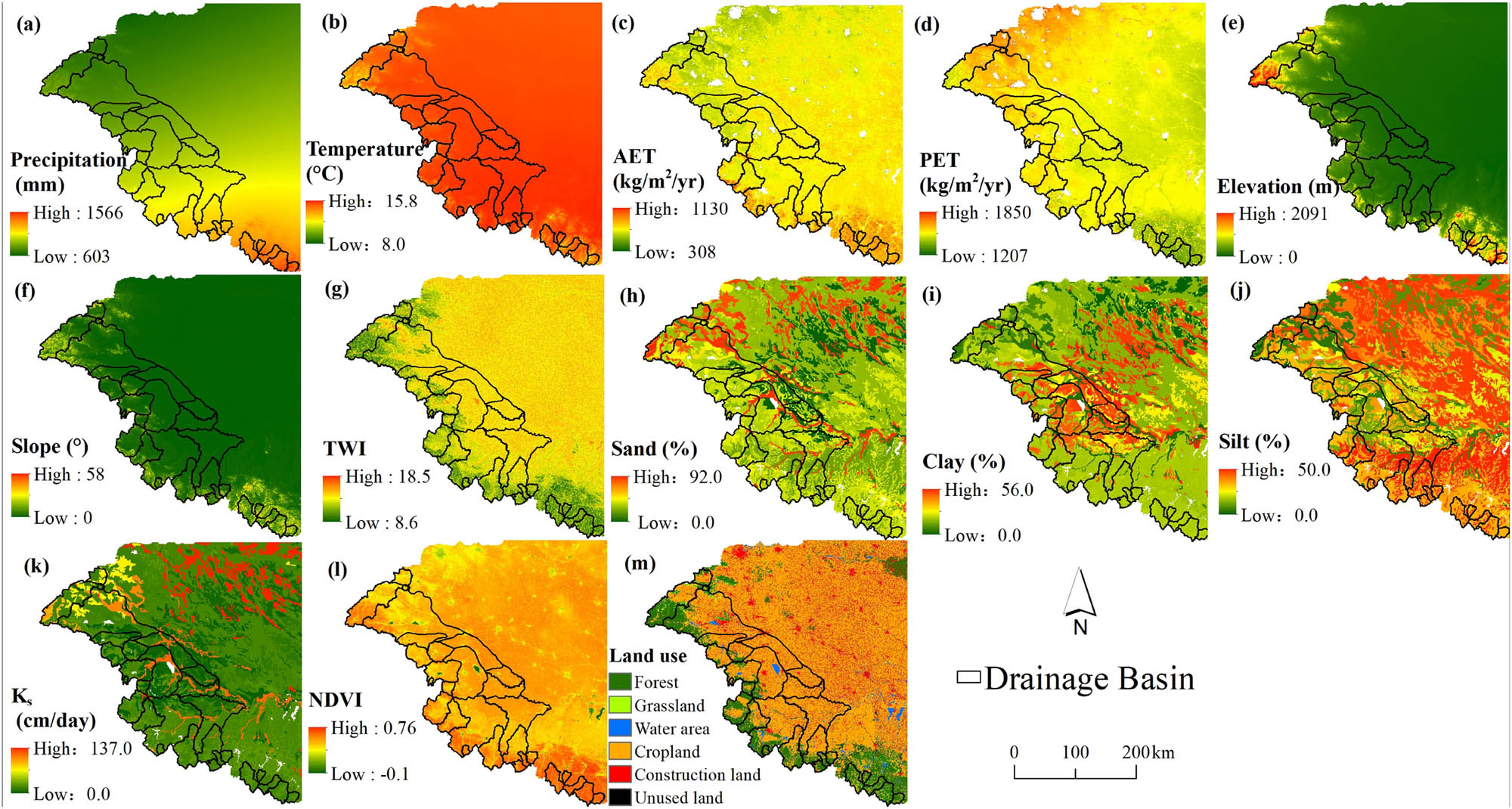
Spatial distributions of 13 driving factors: precipitation (a), temperature (b), AET (c), PET (d), elevation (e), slope (f), TWI (g), sand (h), clay (i), silt (j), K S (k), NDVI (l), and land use (m).
2.3 Water balance equation
For a given basin, the mean annual water balance equation is represented as:
where P, R, and AET are mean annual precipitation, runoff, and AET, respectively. ΔS is the mean annual change in water storage. Over a long period, the amount of water storage is zero. So, RC is represented as
The RC map can be estimated based on the precipitation map and the AET map from remote sensing data.
2.4 Geographical detector
Geographical detector proposed by Wang et al. [29] is a useful statistical method that is not only able to quantitatively detect the relationship between independent variables X and dependent variables Y but it can also be used to investigate the interaction between two independent variables to a dependent variable. Any assumptions of linearity and a specific form of interaction should not be considered. In this study, the factor detector and the interaction detector were adopted to explore the driving factors of the RC in the upper reaches of the Huaihe River Basin. The dependent variable Y was RC, while the independent variable X represented the 13 potential driving factors.
The purpose of the factor detector is to quantitatively detect the explanatory powers of different driving factors of the RC using the q-value. The formula is expressed as
where h = 1, 2,… L is the stratum of factor X (or the variables Y); N and N
h
are the unit numbers of cells in the whole region and the layer h, respectively; and
The interaction detector is used to identify the interactions between two independent variables (X1 and X2) and the dependent variable Y. q(X1 ∩ X2) is calculated and compared with q(X1) and q(X2) to evaluate different relationships (Table 3). There are five possible interaction relationships: nonlinear-weaken, univariate-weaken, independent, bivariate-enhance, and nonlinear-enhance.
Interactions between two explanatory variables
| Description | Interaction |
|---|---|
| q(X1 ∩ X2) < Min(q(X1), q(X2)) | Weaken, nonlinear |
| Min(q(X1), q(X2)) < q(X1 ∩ X2) < Max(q(X1), q(X2)) | Weaken, univariate |
| q(X1 ∩ X2) > Max(q(X1), q(X2)) | Enhance, bivariate |
| q(X1 ∩ X2) = q(X1) + q(X2) | Independent |
| q(X1 ∩ X2) > q(X1) + q(X2) | Enhance, nonlinear |
Note: q(X1) is the q value of variable X1, q(X2) is the q value of variable X2, and q(X1 ∩ X2) is the q value of the interaction between variables X1 and X2.
The geographical detector needs categorical variables as the input data. It is necessary to discretize numerical variables into several strata. It is also important to select discretization methods and divide the number of classifications [36]. Having compared the discretization methods, including the equal interval method, the quantile classification method, and the natural breaks method, the latter was selected to classify these variables into 11 categories as the optimal scheme based on the maximum q value.
3 Results
3.1 Relationships between the RC and driving factors at the watershed scale
The relationships between RC and the 13 driving factors of 29 watersheds are shown in Figure 3. The largest coefficient of determination (R 2) was observed between RC and P (R 2 = 0.826, p = 0.000), which showed a positive trend. The lowest coefficient of determination was found between RC and T (R 2 = 0.049). Both PET and AET greatly influenced on RC. Slope and TWI rather than elevation were the important topographical factors affecting RC. Of 4 soil factors, only silt was significantly correlated with RC (p < 0.01). The proportions of the 3 main land use types were significantly correlated with RC (p < 0.01). Furthermore, RC was more significantly affected by NDVI (R 2 = 0.41, p < 0.01). At the watershed scale, climate was found to predict RC well, followed by topography, land use type, NDVI, and soil.

Scatter plots of runoff coefficient values against precipitation (a), temperature (b), AET (c), PET (d), elevation (e), slope (f), TWI (g), sand (h), clay (i), silt (j), K S (k), NDVI (l), forest (m), cropland (n), and construction land (o) of Shayin River (SYR) (watersheds are indicated by red dots), Hongru River (HRR) (green dots), Huaihe River mainstream (HHRM) (blue dots), and Shipi River (SPR) (yellow dots). The black dashed lines represent the linear regression of all plots.
3.2 Estimating the mean annual RC map
The mean annual precipitation map and the mean annual AET map were used as inputs in the water balance equation to estimate the mean annual RC map of the study area (Figure 4). RC decreased progressively from south to north. RC in the mountain area was higher than in the plain. The estimated RC values of 29 watersheds were extracted (no data pixels were not considered). Figure 5 presents an exponential relationship between estimated RC and actual RC for 29 watersheds, which yielded R 2 and root mean square error (RMSE) of 0.656 and 0.007, respectively. Subsequently, the exponential equation was used to correct the estimated RC map.
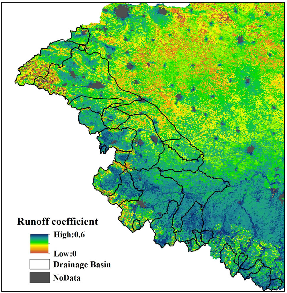
The spatial distribution of mean annual runoff coefficient estimated by the water balance equation across the upper reaches of Huaihe River (no data pixels were covered by surfaces of water body, urban and wetland).

Plots of the estimated and the actual runoff coefficients for Shayin River (SYR) (watersheds are indicated by red dots), Hongru River (HRR) (green dots), Huaihe River mainstream (HHRM) (blue dots), and Shipi River (SPR) (yellow dots). The black dashed line and the black solid line represent the linear and exponential regressions of all plots. R 2: coefficient of determination; RMSE: root mean square error.
Information on 13 driving factors
| Categories | Factor | Abbreviation | Pixel resolution (m) | Unit | Data resource |
|---|---|---|---|---|---|
| Climate | Mean annual precipitation | P | 1,000 | mm | http://www.resdc.cn |
| Mean annual temperature | T | 500 | °C | ||
| Mean annual actual evapotranspiration | AET | 500 | kg/m2/year | https://lpdaac.usgs.gov/ | |
| Mean annual potential evapotranspiration | PET | 500 | kg/m2/year | ||
| Topography | Elevation | Elev | 90 | m | http://www.resdc.cn |
| Slope | Slope | 90 | ° | ||
| Topographic wetness index | TWI | 90 | / | ||
| Soil | Sand percentage | Sand | 1,000 | % | https://iiasa.ac.at/models-and-data/harmonized-world-soil-database |
| Clay percentage | Clay | 1,000 | % | ||
| Silt percentage | Silt | 1,000 | % | ||
| Saturated hydraulic conductivity | K S | 1,000 | cm/day | ||
| Land use | Land use type | LU | 1,000 | Categorical | http://www.resdc.cn |
| Vegetation | Normalized difference vegetation index | NDVI | 1,000 | / | http://www.resdc.cn |
3.3 Relative influences of driving factors on the RC at the pixel scale
3.3.1 The dominant driving factors of the RC
Based on the factor detector model, the q values of 13 driving factors with respect to the spatial patterns of RC in the different river systems were calculated (Table 4). In four different river systems, the q values of AET were the largest factors, exhibiting the highest explanation rates (more than 0.7). The following significant factors were slightly different in the four different river systems. NDVI was the second important driving factor in the Shayin River, Hongru River, and Huaihe River mainstream. The q value of NDVI in the Shipi River was lower, its distribution here had little effect on that of RC. PET, elevation, temperature, and slope are the next most important driving factors. While the main driving factors for the whole study area differed in each river system. The q values of all factors did not exceed 0.3, which were lower than those of an individual river system. P exhibited the highest explanation rates (0.248) of the whole study area, followed by T (0.180), AET (0.154), NDVI (0.141), and elevation (0.137).
Factor detection results for 13 driving factors in different river basins
| Factor type | Factor | SYR | HRR | HHRM | SPR | All |
|---|---|---|---|---|---|---|
| Climate | P | 0.061 | 0.080 | 0.016 | 0.185 | 0.248 |
| T | 0.107 | 0.052 | 0.197 | 0.268 | 0.180 | |
| AET | 0.790 | 0.807 | 0.696 | 0.846 | 0.154 | |
| PET | 0.206 | 0.151 | 0.111 | 0.435 | 0.061 | |
| Soil | Sand | 0.086 | 0.131 | 0.085 | 0.061 | 0.056 |
| Clay | 0.093 | 0.078 | 0.059 | 0.061 | 0.099 | |
| Silt | 0.081 | 0.119 | 0.106 | 0.015 | 0.080 | |
| K S | 0.042 | 0.126 | 0.077 | 0.061 | 0.070 | |
| Topography | Elev | 0.149 | 0.175 | 0.184 | 0.261 | 0.137 |
| slope | 0.121 | 0.114 | 0.136 | 0.070 | 0.056 | |
| TWI | 0.070 | 0.059 | 0.103 | 0.036 | 0.040 | |
| Vegetation | NDVI | 0.253 | 0.297 | 0.314 | 0.020 | 0.141 |
| Land use | LU | 0.096 | 0.004 | 0.111 | 0.017 | 0.019 |
Note: P: mean annual precipitation; T: mean annual temperature; AET: mean annual actual evapotranspiration; PET: mean annual potential evapotranspiration; K S: saturated hydraulic conductivity; Elev: elevation; TWI: topographic wetness index; NDVI: normalized difference vegetation index; LU: land use type.
Overall, RC was found to be primarily influenced by climate-related factors, followed by topographical factors and vegetation. Elevation was the most important factor in the topographical factors. Soil and land use had only a minimal influence on the RC distribution.
3.3.2 Detection of combined influences
The interaction detectors of two environmental factors in the study area were analyzed and the results are shown in Table 5. In five possible interaction relationship types, only nonlinear enhancement and bi-enhancement were observed among the 78 pairs of interactions between 2 factors. The nonlinear enhancement indicates that the q value of the interaction of two factors is greater than the sum of the two factor values. The bi-enhancement effect means that the interactive q value of two factors is larger than that of a single factor. Studies showed that environmental factors had an interactive influence on RC.
Interaction detections between runoff coefficients and 13 driving factors in (a) SYR, (b) HRR, (c) HHRM (d) SPR, and (e) 4 river basins
| P | T | AET | PET | Sand | Clay | Silt | K S | Elev | Slope | TWI | NDVI | |
|---|---|---|---|---|---|---|---|---|---|---|---|---|
| (a) SYR | ||||||||||||
| T | 0.230* | |||||||||||
| AET | 0.907* | 0.824# | ||||||||||
| PET | 0.312* | 0.365* | 0.823# | |||||||||
| Sand | 0.225* | 0.221* | 0.841# | 0.325* | ||||||||
| Clay | 0.190* | 0.223* | 0.856# | 0.336* | 0.143# | |||||||
| Silt | 0.191* | 0.189* | 0.860# | 0.357* | 0.139# | 0.142# | ||||||
| K S | 0.194* | 0.196* | 0.841* | 0.289* | 0.142* | 0.132# | 0.144* | |||||
| Elev | 0.257* | 0.162# | 0.827# | 0.384* | 0.266* | 0.266* | 0.245* | 0.234* | ||||
| Slope | 0.216* | 0.170# | 0.798# | 0.318# | 0.212* | 0.217* | 0.195# | 0.179* | 0.191# | |||
| TWI | 0.161* | 0.148# | 0.796# | 0.286* | 0.171* | 0.173* | 0.155* | 0.127* | 0.176# | 0.143# | ||
| NDVI | 0.317* | 0.310# | 0.805# | 0.320# | 0.328# | 0.3247# | 0.321# | 0.295* | 0.329# | 0.291# | 0.278# | |
| LU | 0.184* | 0.160# | 0.796# | 0.305* | 0.193* | 0.184# | 0.148# | 0.157* | 0.200# | 0.168# | 0.142# | 0.278# |
| (b) HRR | ||||||||||||
| T | 0.238* | |||||||||||
| AET | 0.955* | 0.859# | ||||||||||
| PET | 0.368* | 0.288* | 0.837# | |||||||||
| Sand | 0.251* | 0.204* | 0.825# | 0.259# | ||||||||
| Clay | 0.197* | 0.155* | 0.827# | 0.249* | 0.148# | |||||||
| Silt | 0.254* | 0.184* | 0.825# | 0.256# | 0.148# | 0.148# | ||||||
| K S | 0.234* | 0.191* | 0.826# | 0.251# | 0.147# | 0.148# | 0.144# | |||||
| Elev | 0.312* | 0.235* | 0.813# | 0.281# | 0.255# | 0.250# | 0.251# | 0.246# | ||||
| Slope | 0.207* | 0.164# | 0.814# | 0.256# | 0.216# | 0.185# | 0.201# | 0.206# | 0.219# | |||
| TWI | 0.149* | 0.128* | 0.813# | 0.230* | 0.178# | 0.148* | 0.168# | 0.171# | 0.193# | 0.136# | ||
| NDVI | 0.400* | 0.338# | 0.826# | 0.358# | 0.365# | 0.352# | 0.352# | 0.366# | 0.353# | 0.329# | 0.320# | |
| LU | 0.089* | 0.089* | 0.811* | 0.215* | 0.148* | 0.115* | 0.141* | 0.151* | 0.192* | 0.134* | 0.083* | 0.306* |
| (c) HHRM | ||||||||||||
| T | 0.281* | |||||||||||
| AET | 0.944* | 0.730# | ||||||||||
| PET | 0.185* | 0.341* | 0.740# | |||||||||
| Sand | 0.128* | 0.249* | 0.766# | 0.196* | ||||||||
| Clay | 0.094* | 0.264* | 0.778* | 0.179* | 0.113# | |||||||
| Silt | 0.150* | 0.265# | 0.809* | 0.224* | 0.121# | 0.126# | ||||||
| K S | 0.119* | 0.256# | 0.752# | 0.188* | 0.119# | 0.103# | 0.125# | |||||
| Elev | 0.285* | 0.225# | 0.730# | 0.330* | 0.245# | 0.258* | 0.255# | 0.241# | ||||
| Slope | 0.220* | 0.223# | 0.730# | 0.283* | 0.210# | 0.207* | 0.216# | 0.195# | 0.205# | |||
| TWI | 0.165* | 0.225# | 0.726# | 0.230* | 0.177# | 0.166* | 0.186# | 0.160# | 0.205# | 0.157# | ||
| NDVI | 0.384* | 0.354# | 0.745# | 0.415# | 0.351# | 0.347# | 0.358# | 0.337# | 0.341# | 0.326# | 0.323# | |
| (d) SPR | ||||||||||||
| T | 0.296# | |||||||||||
| AET | 0.916# | 0.930# | ||||||||||
| PET | 0.522# | 0.585# | 0.860# | |||||||||
| Sand | 0.202# | 0.282# | 0.865# | 0.462# | ||||||||
| Clay | 0.202# | 0.286# | 0.868# | 0.467# | 0.061# | |||||||
| Silt | 0.193# | 0.284* | 0.856# | 0.447# | 0.062# | 0.062# | ||||||
| K S | 0.202# | 0.281# | 0.865# | 0.462# | 0.062# | 0.062# | 0.062# | |||||
| Elev | 0.285# | 0.288# | 0.929# | 0.578# | 0.271# | 0.272# | 0.276* | 0.271# | ||||
| Slope | 0.209# | 0.285# | 0.863# | 0.473# | 0.123# | 0.116# | 0.099* | 0.122# | 0.286# | |||
| TWI | 0.206# | 0.292# | 0.853# | 0.454# | 0.099* | 0.099* | 0.061* | 0.099* | 0.284# | 0.095# | ||
| NDVI | 0.216* | 0.325* | 0.851# | 0.450# | 0.088* | 0.090* | 0.045* | 0.087* | 0.312* | 0.116* | 0.077* | |
| LU | 0.197# | 0.283# | 0.852# | 0.448# | 0.078# | 0.079* | 0.041* | 0.078# | 0.273# | 0.088* | 0.057* | 0.049* |
| (e) Four river basins | ||||||||||||
| T | 0.400# | |||||||||||
| AET | 0.948* | 0.568* | ||||||||||
| PET | 0.428* | 0.374* | 0.400* | |||||||||
| Sand | 0.350# | 0.301# | 0.402* | 0.212* | ||||||||
| Clay | 0.316# | 0.276# | 0.409* | 0.202* | 0.189# | |||||||
| Silt | 0.345* | 0.297* | 0.375* | 0.184* | 0.163# | 0.152# | ||||||
| K S | 0.335* | 0.279* | 0.345* | 0.178* | 0.168# | 0.183* | 0.174* | |||||
| Elev | 0.431* | 0.276* | 0.332* | 0.203* | 0.232* | 0.208* | 0.197* | 0.184* | ||||
| Slope | 0.368* | 0.245* | 0.270* | 0.174* | 0.199* | 0.173* | 0.157* | 0.157* | 0.108# | |||
| TWI | 0.326* | 0.227* | 0.239* | 0.144* | 0.178* | 0.148* | 0.136* | 0.130* | 0.099* | 0.079# | ||
| NDVI | 0.490* | 0.372* | 0.295# | 0.285* | 0.260# | 0.254# | 0.228* | 0.228* | 0.254* | 0.192# | 0.173# | |
| LU | 0.309* | 0.199* | 0.197* | 0.120* | 0.172* | 0.137* | 0.113* | 0.118* | 0.073# | 0.068# | 0.061* | 0.159# |
Note: # indicates that the interaction is a bi-enhancement; * indicates that the interaction is nonlinear-enhancement.
Note: P: mean annual precipitation; T: mean annual temperature; AET: mean annual actual evapotranspiration; PET: mean annual potential evapotranspiration; K S: saturated hydraulic conductivity; Elev: elevation; TWI: topographic wetness index; NDVI: normalized difference vegetation index.
As regards interaction effects between factors in the Shayin River, Hongru River, Huaihe River mainstream, and Shipi River (Table 5a–d), the percentages of interaction pairs of the nonlinear-enhancement effect were 53, 42, 36, and 27%, respectively, mainly concentrated on the lower q value factors, such as P, LU, and NDVI. Four river basins had similar results wherein the interactions between AET and any other factors were the most prominent. The interaction effect between P and AET (P ∩ AET) had the strongest effect on RC, which exceeded 0.900.
Across the whole study area, 76% of pairs showed the nonlinear-enhance effect (Table 5e). The top five interactions between factors were P ∩ T (0.948), AET ∩ T (0.568), P ∩ NDVI (0.490), P ∩ Elev (0.431), and P ∩ PET (0.428). This indicates that climate factors (P, T, AET, and PET), NDVI, and elevation had the greatest impact on the RC values.
4 Discussion
4.1 The RC map
The water balance equation was used to produce a RC map using the mean annual precipitation and the mean annual AET. The mean annual precipitation map came from the spatial interpolation technique using meteorological observation data. The mean annual AET map came from Moderate resolution imaging spectroradiometer (MODIS) global ET products which reached 86% accuracy evaluated by global flux measurement data [11]. Several studies have shown that MODIS ET data could be used for calibrating biophysical models [37], analyzing ET at different temporal and spatial scales [38], computing monthly water balance components [39], and estimating mean runoff over the years [15]. In this study, the mean estimation RC of 29 watersheds was 0.39, close to the actual RC of 0.37. A fairly significant exponential relationship was observed between estimated RC and actual RC from 29 watersheds (Figure 5). The estimated RC values in the Shayin River were higher than the actual RC values, while the estimated RC values in the Shipi River were lower. The main reason is that the MOD16 ET was overestimated from north to south in Chinese river basins [40]. The uncertainties of MODIS ET data were mostly seen in forests and mountains [41]. It is possible that the MODIS ET product did not take into account the topographical relief condition because of the algorithm limitations and uncertainties from input data [11]. It should be noted that RC values in the regions of water body, wetland, and urban and built-up areas could not be estimated. The main reason is that MOD16A3 ET products used MODIS Leaf area index (LAI) and Fraction of photosynthetically active radiation (FPAR) products (MOD15) as the input data. Non-vegetated pixels in these regions could not calculate LAI/FPAR.
4.2 Driving forces of the RC
Climate and watershed characteristics both control the hydrological process of a watershed and determine the RC. The main driving factors of the RCs could be related to scale. The geographical detector is a spatial statistical method to assess the relationships of different geographical strata and reveal the driving forces behind spatial variations [42,43,44].
Climate is the main factor controlling the water cycle [22,45]. The spatial variabilities of climate factors caused significant changes in our study. Precipitation, temperature, and AET decreased from south to north. The RC values of the 29 watersheds also declined from south to north in the study area. High precipitation makes increased runoff more likely. Precipitation proved to be the most important variable for the RC at the watershed scale and across the whole study area. By contrast, at the scale of a single river basin or smaller, the dominant factor which exhibited the highest explanation rate was AET. The main reason is that the spatial variation of precipitation in a small region is relatively slight. In the temperate and subtropical monsoon climate zones, precipitation and evapotranspiration were the main factors affecting runoff [20].
Topography also exerts a strong influence on hydrological processes [25]. Of the topographical variables considered in this study, slope and TWI were more important than elevation at the watershed scale mainly because they could affect the movement of water across watersheds. Mean basin slope could be used to predict RC in various environments [46]. TWI is used to calculate topographic control on wetness and runoff. Runoff generation can be modeled using TWI [47,48]. By contrast, from the watershed scale to the pixel scale, elevation was the most important topographical variable.
NDVI can be used as an important factor to regulate water resources both at the watershed scale and at the pixel scale. NDVI had higher q values. NDVI is a comprehensive reflection of climate, topography, land use, and soil [20]. Higher NDVI values were mainly distributed in forest and mountain regions. The forest density variable was one of the most important factors in predicting the RC [23].
The RC was also found to be highly influenced by land use at the watershed scale. The RC generally increased with an increase in the forest coverage. On the one hand, forest areas can hold more water and produce more runoff than other land use types [30,49]. On the other hand, in this study area, the forest is generally located in mountainous areas, where precipitation is more than 1,024 mm. Cropland coverage was negatively associated with the RC, because of low elevation and precipitation interception. In addition, the irrigation of croplands in the study area primarily uses water from the river systems [49]. Construction land was found to have a negative effect on runoff generation at the watershed scale (Figure 3o), which was not consistent with previous studies [50,51,52]. Some studies found that there is a threshold effect of the impervious area on the RC. When the percentage of construction land area was more than 10% [53] or 20% [50], the construction land area would have an impact on the RC. This study’s largest percentage of construction land areas is less than 18%. The proportion of forest had a significant negative correlation with the construction land. Therefore, forest coverage was the most important land cover type on the RC.
However, land use types were found to have less effect on the RC at the pixel scale. The q values of land use were low. Soil factors and the land use type had only a minimal influence on RC distribution. Soil properties did not seem to exert a major influence on RC. Only silt content was highly correlated with RC (p < 0.01). Moreover, the q values of soil properties were low. Land use, soil types, and geology had a minor control on RCs of the watersheds [24].
4.3 Analysis of interaction between factors
Given that the interactions between different driving factors and the RC are complicated, the interaction detector was used to analyze the interactions between any two driving factors. The interaction results indicated that the explanatory powers of any two-factor interaction on the RC was higher than the q values of a single factor, indicating that the spatial heterogeneity of the RC was largely affected by interactions between factors. Climate and watershed characteristics explained the variation in the RC [30].
4.4 Limitations
There are several limitations to the current study. First, remote sensing products can predict RC at the watershed scale, but uncertainties and accuracies of these products should be considered. MOD16 ET products are inevitably subject to errors resulting from input data and retrieval algorithms. Evaporation on different surfaces can create significant variations. Second, RC values in the construction land could not be estimated. It is feasible to estimate the impervious surface area from remote sensing images and simulate surface runoff by the soil conservation service curve number method [52,54]. Third, the interactions among three or more factors should be further explored in the future. Fourth, numerous factors affecting the runoff and those that predominate in different climatic conditions vary. Their interactive influences can be extremely complex.
5 Conclusion
The spatially distributed RC map was produced based on remote sensing data from the upper reaches of the Huaihe River Basin. The estimated RCs of 29 watersheds showed an exponential relationship with actual RCs (R 2 = 0.656, RMSE = 0.007). Using remote sensing data to estimate the RC map is promising, especially in ungauged catchments. Based on the analysis of the influence of four climate factors (precipitation, temperature, AET, and PET) and nine watershed properties (elevation, slope, TWI, sand, clay, silt, saturated hydraulic conductivity, NDVI, and land use) on the RC, the differences among these influencing factors driving RC at the different scales were quantified. At the watershed scale, RC increased linearly with precipitation. PET, AET, slope, TWI, silt, and the areal percentage of forest were found to be significantly correlated with RC. At the pixel scale, the geographical detector was used to identify the driving factors of the RC and their interactions. The top five factors influencing the RC in the whole study area were precipitation, temperature, AET, NDVI, and elevation, whose explanatory powers were 0.248, 0.180, 0.154, 0.141, and 0.137, respectively. While in four different river systems, AET had the top explanation rate, and the following significant factors were slightly different. Results of detection of interactions show that any two factors had a nonlinear or bilinear enhanced effect on the RC. The most influential synergistic groups were climate factors with other factors. Our findings could be useful in selecting suitable factors for predicting RC. And using the nonlinear approaches may predict RC better than the linear approaches. This study provides a reference to disentangle the complicated driving factors of RC and to understand the rainfall-runoff response in other basins. In the future, we plan to produce the RC map using different remote sensing data, quantify the effects of climate and watershed factors on runoff in different climatic regions, and understand the water balance response mechanism of watersheds.
Acknowledgements
This work is supported in part by the National Natural Science Foundation of China (NO. 41801075), China Postdoctoral Science Foundation (NO. 2018M642349) and Huai’an Municipal Science and Technology Bureau (NO. HAB202159). We thank the editor and anonymous reviewers for their insightful comments.
-
Author contributions: X.L.: conceptualization; X.L. and N.Y.: methodology; Q.H.: formal analysis; X.L. and N.Y.: writing – original draft preparation; Q.H. and H.W.: writing – review and editing; Q.H. and H.W.: supervision; X.L. and N.Y.: funding acquisition. All authors have read and agreed to the published version of the manuscript.
-
Conflict of interest: The authors declare no conflict of interest.
-
Data availability statement: The data used to support the findings of the present study are available from the corresponding author upon request.
References
[1] Zhang Z, Chen X, Huang Y, Zhang Y. Effect of catchment properties on runoff coefficient in a karst area of southwest China. Hydrol Process. 2014;28(11):3691–702. 10.1002/hyp.9920.Search in Google Scholar
[2] Chen T, Hsu W, Chen W. An assessment of water resources in the Taiwan strait island using the water poverty index. Sustainability. 2020;12(6):2351. 10.3390/su12062351.Search in Google Scholar
[3] Birkinshaw SJ, O’Donnell G, Glenis V, Kilsby C. Improved hydrological modelling of urban catchments using runoff coefficients. J Hydrol. 2021;594:125884. 10.1016/j.jhydrol.2020.125884.Search in Google Scholar
[4] Gu X, Yang G, He X, Zhao L, Li X, Li P, et al. Hydrological process simulation in Manas River Basin using CMADS. Open Geosci. 2020;12(1):946–57. 10.1515/geo-2020-0127.Search in Google Scholar
[5] Parajka J, Viglione A, Rogger M, Salinas JL, Sivapalan M, Blöschl G. Comparative assessment of predictions in ungauged basins – Part 1: Runoff-hydrograph studies. Hydrol Earth Syst Sc. 2013;17(5):1783–95. 10.5194/hess-17-1783-2013.Search in Google Scholar
[6] Hrachowitz M, Savenije HHG, Blöschl G, McDonnell JJ, Sivapalan M, Pomeroy JW, et al. A decade of predictions in ungauged basins (PUB)–a review. Hydrological Sci J. 2013;58(6):1198–255. 10.1080/02626667.2013.803183.Search in Google Scholar
[7] Wu Z, Xu Z, Wang F, He H, Zhou J, Wu X, et al. Hydrologic evaluation of multi-source satellite precipitation products for the Upper Huaihe River Basin, China. Remote Sens. 2018;10(6):840. 10.3390/rs10060840.Search in Google Scholar
[8] Ashouri H, Hsu K, Sorooshian S, Braithwaite DK, Knapp KR, Cecil LD, et al. PERSIANN-CDR: Daily precipitation climate data record from multisatellite observations for hydrological and climate studies. B Am Meteorol Soc. 2015;96(1):69–83. 10.1175/BAMS-D-13-00068.1.Search in Google Scholar
[9] Crow WT, Chen F, Reichle RH, Xia Y. Diagnosing bias in modeled soil moisture/runoff coefficient correlation using the SMAP Level 4 soil moisture product. Water Resour Res. 2019;55(8):7010–26. 10.1029/2019WR025245.Search in Google Scholar
[10] Gruber A, Scanlon T, van der Schalie R, Wagner W, Dorigo W. Evolution of the ESA CCI soil moisture climate data records and their underlying merging methodology. Earth Syst Sci Data. 2019;11(2):717–39. 10.5194/essd-11-717-2019.Search in Google Scholar
[11] Mu Q, Zhao M, Running SW. Improvements to a MODIS global terrestrial evapotranspiration algorithm. Remote Sens Environ. 2011;115(8):1781–800. 10.1016/j.rse.2011.02.019.Search in Google Scholar
[12] Miralles DG, Holmes TRH, De Jeu RAM, Gash JH, Meesters AGCA, Dolman AJ. Global land-surface evaporation estimated from satellite-based observations. Hydrol Earth Syst Sc. 2011;15(2):453–69. 10.5194/hess-15-453-2011.Search in Google Scholar
[13] Crowley JW, Mitrovica JX, Bailey RC, Tamisiea ME, Davis JL. Land water storage within the Congo Basin inferred from GRACE satellite gravity data. Geophys Res Lett. 2006;33(19):L19402. 10.1029/2006GL027070.Search in Google Scholar
[14] Hong Y, Adler RF, Hossain F, Curtis S, Huffman GJ. A first approach to global runoff simulation using satellite rainfall estimation. Water Resour Res. 2007;43(8):W08502. 10.1029/2006WR005739.Search in Google Scholar
[15] Gwate O, Mantel SK, Gibson LA, Munch Z, Palmer AR. Exploring dynamics of evapotranspiration in selected land cover classes in a sub-humid grassland: A case study in quaternary catchment S50E, South Africa. J Arid Environ. 2018;157:66–76. 10.1016/j.jaridenv.2018.05.011.Search in Google Scholar
[16] Chen B, Krajewski WF, Helmers MJ, Zhang Z. Spatial variability and temporal persistence of event runoff coefficients for cropland hillslopes. Water Resour Res. 2019;55(2):1583–97. 10.1029/2018wr023576.Search in Google Scholar
[17] Yan J, Jia S, Lv A, Zhu W. Water resources assessment of china’s transboundary River Basins using a machine learning approach. Water Resour Res. 2019;55(1):632–55. 10.1029/2018WR023044.Search in Google Scholar
[18] Kim N, Shin M. Estimation of peak flow in ungauged catchments using the relationship between runoff coefficient and curve number. Water. 2018;10(11):1669. 10.3390/w10111669.Search in Google Scholar
[19] Sriwongsitanon N, Taesombat W. Effects of land cover on runoff coefficient. J Hydrol. 2011;410(3–4):226–38. 10.1016/j.jhydrol.2011.09.021.Search in Google Scholar
[20] Huo J, Liu C, Yu X, Jia G, Chen L. Effects of watershed char and climate variables on annual runoff in different climatic zones in China. Sci Total Env. 2021;754:142157. 10.1016/j.scitotenv.2020.142157.Search in Google Scholar PubMed
[21] Liu W, Li Z, Zhu J, Xu C, Xu X. Dominant factors controlling runoff coefficients in karst watersheds. J Hydrol. 2020;590:125486. 10.1016/j.jhydrol.2020.125486.Search in Google Scholar
[22] Norbiato D, Borga M, Merz R, Blöschl G, Carton A. Controls on event runoff coefficients in the eastern Italian Alps. J Hydrol. 2009;375(3):312–25. 10.1016/j.jhydrol.2009.06.044.Search in Google Scholar
[23] Li M, Zhang Y, Wallace J, Campbell E. Estimating annual runoff in response to forest change: A statistical method based on random forest. J Hydrol. 2020;589:125168. 10.1016/j.jhydrol.2020.125168.Search in Google Scholar
[24] Merz R, Blöschl G. A regional analysis of event runoff coefficients with respect to climate and catchment characteristics in Austria. Water Resour Res. 2009;45:W01405. 10.1029/2008WR007163.Search in Google Scholar
[25] Cai S, Geng H, Pan B, Hong Y, Chen L. Topographic controls on the annual runoff coefficient and implications for landscape evolution across semiarid Qilian Mountains, NE Tibetan Plateau. J Mt Sci Engl. 2020;17(2):464–79. 10.1007/s11629-019-5584-7.Search in Google Scholar
[26] Cerdan O, Le Bissonnais Y, Govers G, Lecomte V, van Oost K, Couturier A, et al. Scale effect on runoff from experimental plots to catchments in agricultural areas in Normandy. J Hydrol. 2004;299(1–2):4–14. 10.1016/j.jhydrol.2004.02.017.Search in Google Scholar
[27] Zhang Q, Liu J, Yu X, Chen L. Scale effects on runoff and a decomposition analysis of the main driving factors in Haihe Basin mountainous area. Sci Total Environ. 2019;690:1089–99. 10.1016/j.scitotenv.2019.06.540.Search in Google Scholar PubMed
[28] Tian W, Bai P, Wang K, Liang K, Liu C. Simulating the change of precipitation-runoff relationship during drought years in the eastern monsoon region of China. Sci Total Environ. 2020;723:138172. 10.1016/j.scitotenv.2020.138172.Search in Google Scholar PubMed
[29] Wang JF, Li XH, Christakos G, Liao YL, Zhang T, Gu X, et al. Geographical detectors‐based health risk assessment and its application in the neural tube defects study of the Heshun Region, China. Int J Geogr Inf Sci. 2010;24(1):107–27. 10.1080/13658810802443457.Search in Google Scholar
[30] Liu Y, Cao X, Li T. Identifying driving forces of built-up land expansion based on the geographical detector: a case study of pearl river delta Urban agglomeration. Int J Environ Res Public Health. 2020;17(5):1759. 10.3390/ijerph17051759.Search in Google Scholar PubMed PubMed Central
[31] Wu W, Zhang M, Ding Y. Exploring the effect of economic and environment factors on PM2.5 concentration: A case study of the Beijing-Tianjin-Hebei region. J Environ Manage. 2020;268:110703. 10.1016/j.jenvman.2020.110703.Search in Google Scholar PubMed
[32] Xu E, Zhang H. Change pathway and intersection of rainfall, soil, and land use influencing water-related soil erosion. Ecol Indic. 2020;113:106281. 10.1016/j.ecolind.2020.106281.Search in Google Scholar
[33] Wang J, Hu M, Zhang F, Gao B. Influential factors detection for surface water quality with geographical detectors in China. Stoch Environ Res Risk Assess. 2018;32(9):2633–45. 10.1007/s00477-018-1532-2.Search in Google Scholar
[34] Nachtergaele F, van Velthuizen H, Verelst L, Batjes N, Dijkshoorn K, van Engelen V, et al. Harmonized world soil database. Wageningen: ISRIC; 2009. http://library.wur.nl/WebQuery/file/isric/fulltext/isricu_t4bb310b7_001.pdf.Search in Google Scholar
[35] Dai Y, Shangguan W, Duan Q, Liu B, Fu S, Niu G. Development of a China dataset of soil hydraulic parameters using pedotransfer functions for land surface modeling. J Hydrometeorol. 2013;14(3):869–87. 10.1175/JHM-D-12-0149.1.Search in Google Scholar
[36] Cao F, Ge Y, Wang J. Optimal discretization for geographical detectors-based risk assessment. GISci Remote Sens. 2013;50(1):78–92. 10.1080/15481603.2013.778562.Search in Google Scholar
[37] Dile YT, Ayana EK, Worqlul AW, Xie H, Srinivasan R, Lefore N, et al. Evaluating satellite-based evapotranspiration estimates for hydrological applications in data-scarce regions: A case in Ethiopia. Sci Total Environ. 2020;743:140702. 10.1016/j.scitotenv.2020.140702.Search in Google Scholar PubMed
[38] Jia Z, Liu S, Xu Z, Chen Y, Zhu M. Validation of remotely sensed evapotranspiration over the Hai River Basin, China. J Geophys Res Atmos. 2012;117:D13113. 10.1029/2011JD017037.Search in Google Scholar
[39] Falalakis G, Gemitzi A. A simple method for water balance estimation based on the empirical method and remotely sensed evapotranspiration estimates. J Hydroinform. 2020;22(2):440–51. 10.2166/hydro.2020.182.Search in Google Scholar
[40] Jiang Y, Wang W, Zhou Z. Evaluation of MODIS MOD16 evaportranspiration product in Chinese river basins. J Nat Res 2017:32(3):517–28 (in Chinese with an English abstract). 10.11849/zrzyxb.20160440.Search in Google Scholar
[41] Mu Q, Heinsch FA, Zhao M, Running SW. Development of a global evapotranspiration algorithm based on MODIS and global meteorology data. Remote Sens Environ. 2007;111(4):519–36. 10.1016/j.rse.2007.04.015.Search in Google Scholar
[42] Hu D, Meng Q, Zhang L, Zhang Y. Spatial quantitative analysis of the potential driving factors of land surface temperature in different “Centers” of polycentric cities: A case study in Tianjin, China. Sci Total Environ. 2020;706:135244. 10.1016/j.scitotenv.2019.135244.Search in Google Scholar PubMed
[43] Zhao S, Li W, Zhao K, Zhang P. Change characteristics and multilevel influencing factors of real estate inventory–case studies from 35 key cities in China. Land. 2021;10(9):928. 10.3390/land10090928.Search in Google Scholar
[44] Li J, Wang J, Zhang J, Liu C, He S, Liu L. Growing-season vegetation coverage patterns and driving factors in the China-Myanmar economic corridor based on google earth engine and geographic detector. Ecol Indic. 2022;136:108620. 10.1016/j.ecolind.2022.108620.Search in Google Scholar
[45] Merz R, Blöschl G, Parajka J. Spatio-temporal variability of event runoff coefficients. J Hydrol. 2006;331(3–4):591–604. 10.1016/j.jhydrol.2006.06.008.Search in Google Scholar
[46] Chang H, Johnson G, Hinkley T, Jung I. Spatial analysis of annual runoff ratios and their variability across the contiguous U.S. J Hydrol. 2014;511:387–402. 10.1016/j.jhydrol.2014.01.066.Search in Google Scholar
[47] Quinn PF, Beven KJ, Lamb R. The in(a/tan/β) index: How to calculate it and how to use it within the topmodel framework. Hydrol Process. 1995;9(2):161–82. 10.1002/hyp.3360090204.Search in Google Scholar
[48] Lane SN, Brookes CJ, Kirkby MJ, Holden J. A network-index-based version of TOPMODEL for use with high-resolution digital topographic data. Hydrol Process. 2004;18(1):191–201. 10.1002/hyp.5208.Search in Google Scholar
[49] Wang G, Yang H, Wang L, Xu Z, Xue B. Using the SWAT model to assess impacts of land use changes on runoff generation in headwaters. Hydrol Process. 2014;28(3):1032–42. 10.1002/hyp.9645.Search in Google Scholar
[50] Goldshleger N, Shoshany M, Karnibad L, Arbel S, Getker M. Generalising relationships between runoff-rainfall coefficients and impervious areas: An integration of data from case studies in Israel with data sets from Australia and the USA. Urban Water J 2009;6(3):201–8. 10.1080/15730620802246355.Search in Google Scholar
[51] Shuster WD, Bonta J, Thurston H, Warnemuende E, Smith DR. Impacts of impervious surface on watershed hydrology: A review. Urban Water J. 2005;2(4):263–75. 10.1080/15730620500386529.Search in Google Scholar
[52] Xu C, Rahman M, Haase D, Wu Y, Su M, Pauleit S. Surface runoff in urban areas: The role of residential cover and urban growth form. J Clean Prod. 2020;262:121421. 10.1016/j.jclepro.2020.121421.Search in Google Scholar
[53] Oudin L, Salavati B, Furusho-Percot C, Ribstein P, Saadi M. Hydrological impacts of urbanization at the catchment scale. J Hydrol. 2018;559:774–86. 10.1016/j.jhydrol.2018.02.064.Search in Google Scholar
[54] Ibrahim S, Brasi B, Yu Q, Siddig M. Curve number estimation using rainfall and runoff data from five catchments in Sudan. Open Geosci. 2022;14(1):294–303. 10.1515/geo-2022-0356.Search in Google Scholar
© 2022 the author(s), published by De Gruyter
This work is licensed under the Creative Commons Attribution 4.0 International License.
Articles in the same Issue
- Regular Articles
- Study on observation system of seismic forward prospecting in tunnel: A case on tailrace tunnel of Wudongde hydropower station
- The behaviour of stress variation in sandy soil
- Research on the current situation of rural tourism in southern Fujian in China after the COVID-19 epidemic
- Late Triassic–Early Jurassic paleogeomorphic characteristics and hydrocarbon potential of the Ordos Basin, China, a case of study of the Jiyuan area
- Application of X-ray fluorescence mapping in turbiditic sandstones, Huai Bo Khong Formation of Nam Pat Group, Thailand
- Fractal expression of soil particle-size distribution at the basin scale
- Study on the changes in vegetation structural coverage and its response mechanism to hydrology
- Spatial distribution analysis of seismic activity based on GMI, LMI, and LISA in China
- Rock mass structural surface trace extraction based on transfer learning
- Hydrochemical characteristics and D–O–Sr isotopes of groundwater and surface water in the northern Longzi county of southern Tibet (southwestern China)
- Insights into origins of the natural gas in the Lower Paleozoic of Ordos basin, China
- Research on comprehensive benefits and reasonable selection of marine resources development types
- Embedded deformation of the rubble-mound foundation of gravity-type quay walls and influence factors
- Activation of Ad Damm shear zone, western Saudi Arabian margin, and its relation to the Red Sea rift system
- A mathematical conjecture associates Martian TARs with sand ripples
- Study on spatio-temporal characteristics of earthquakes in southwest China based on z-value
- Sedimentary facies characterization of forced regression in the Pearl River Mouth basin
- High-precision remote sensing mapping of aeolian sand landforms based on deep learning algorithms
- Experimental study on reservoir characteristics and oil-bearing properties of Chang 7 lacustrine oil shale in Yan’an area, China
- Estimating the volume of the 1978 Rissa quick clay landslide in Central Norway using historical aerial imagery
- Spatial accessibility between commercial and ecological spaces: A case study in Beijing, China
- Curve number estimation using rainfall and runoff data from five catchments in Sudan
- Urban green service equity in Xiamen based on network analysis and concentration degree of resources
- Spatio-temporal analysis of East Asian seismic zones based on multifractal theory
- Delineation of structural lineaments of Southeast Nigeria using high resolution aeromagnetic data
- 3D marine controlled-source electromagnetic modeling using an edge-based finite element method with a block Krylov iterative solver
- A comprehensive evaluation method for topographic correction model of remote sensing image based on entropy weight method
- Quantitative discrimination of the influences of climate change and human activity on rocky desertification based on a novel feature space model
- Assessment of climatic conditions for tourism in Xinjiang, China
- Attractiveness index of national marine parks: A study on national marine parks in coastal areas of East China Sea
- Effect of brackish water irrigation on the movement of water and salt in salinized soil
- Mapping paddy rice and rice phenology with Sentinel-1 SAR time series using a unified dynamic programming framework
- Analyzing the characteristics of land use distribution in typical village transects at Chinese Loess Plateau based on topographical factors
- Management status and policy direction of submerged marine debris for improvement of port environment in Korea
- Influence of Three Gorges Dam on earthquakes based on GRACE gravity field
- Comparative study of estimating the Curie point depth and heat flow using potential magnetic data
- The spatial prediction and optimization of production-living-ecological space based on Markov–PLUS model: A case study of Yunnan Province
- Major, trace and platinum-group element geochemistry of harzburgites and chromitites from Fuchuan, China, and its geological significance
- Vertical distribution of STN and STP in watershed of loess hilly region
- Hyperspectral denoising based on the principal component low-rank tensor decomposition
- Evaluation of fractures using conventional and FMI logs, and 3D seismic interpretation in continental tight sandstone reservoir
- U–Pb zircon dating of the Paleoproterozoic khondalite series in the northeastern Helanshan region and its geological significance
- Quantitatively determine the dominant driving factors of the spatial-temporal changes of vegetation-impacts of global change and human activity
- Can cultural tourism resources become a development feature helping rural areas to revitalize the local economy under the epidemic? An exploration of the perspective of attractiveness, satisfaction, and willingness by the revisit of Hakka cultural tourism
- A 3D empirical model of standard compaction curve for Thailand shales: Porosity in function of burial depth and geological time
- Attribution identification of terrestrial ecosystem evolution in the Yellow River Basin
- An intelligent approach for reservoir quality evaluation in tight sandstone reservoir using gradient boosting decision tree algorithm
- Detection of sub-surface fractures based on filtering, modeling, and interpreting aeromagnetic data in the Deng Deng – Garga Sarali area, Eastern Cameroon
- Influence of heterogeneity on fluid property variations in carbonate reservoirs with multistage hydrocarbon accumulation: A case study of the Khasib formation, Cretaceous, AB oilfield, southern Iraq
- Designing teaching materials with disaster maps and evaluating its effectiveness for primary students
- Assessment of the bender element sensors to measure seismic wave velocity of soils in the physical model
- Appropriated protection time and region for Qinghai–Tibet Plateau grassland
- Identification of high-temperature targets in remote sensing based on correspondence analysis
- Influence of differential diagenesis on pore evolution of the sandy conglomerate reservoir in different structural units: A case study of the Upper Permian Wutonggou Formation in eastern Junggar Basin, NW China
- Planting in ecologically solidified soil and its use
- National and regional-scale landslide indicators and indexes: Applications in Italy
- Occurrence of yttrium in the Zhijin phosphorus deposit in Guizhou Province, China
- The response of Chudao’s beach to typhoon “Lekima” (No. 1909)
- Soil wind erosion resistance analysis for soft rock and sand compound soil: A case study for the Mu Us Sandy Land, China
- Investigation into the pore structures and CH4 adsorption capacities of clay minerals in coal reservoirs in the Yangquan Mining District, North China
- Overview of eco-environmental impact of Xiaolangdi Water Conservancy Hub on the Yellow River
- Response of extreme precipitation to climatic warming in the Weihe river basin, China and its mechanism
- Analysis of land use change on urban landscape patterns in Northwest China: A case study of Xi’an city
- Optimization of interpolation parameters based on statistical experiment
- Late Cretaceous adakitic intrusive rocks in the Laimailang area, Gangdese batholith: Implications for the Neo-Tethyan Ocean subduction
- Tectonic evolution of the Eocene–Oligocene Lushi Basin in the eastern Qinling belt, Central China: Insights from paleomagnetic constraints
- Geographic and cartographic inconsistency factors among different cropland classification datasets: A field validation case in Cambodia
- Distribution of large- and medium-scale loess landslides induced by the Haiyuan Earthquake in 1920 based on field investigation and interpretation of satellite images
- Numerical simulation of impact and entrainment behaviors of debris flow by using SPH–DEM–FEM coupling method
- Study on the evaluation method and application of logging irreducible water saturation in tight sandstone reservoirs
- Geochemical characteristics and genesis of natural gas in the Upper Triassic Xujiahe Formation in the Sichuan Basin
- Wehrlite xenoliths and petrogenetic implications, Hosséré Do Guessa volcano, Adamawa plateau, Cameroon
- Changes in landscape pattern and ecological service value as land use evolves in the Manas River Basin
- Spatial structure-preserving and conflict-avoiding methods for point settlement selection
- Fission characteristics of heavy metal intrusion into rocks based on hydrolysis
- Sequence stratigraphic filling model of the Cretaceous in the western Tabei Uplift, Tarim Basin, NW China
- Fractal analysis of structural characteristics and prospecting of the Luanchuan polymetallic mining district, China
- Spatial and temporal variations of vegetation coverage and their driving factors following gully control and land consolidation in Loess Plateau, China
- Assessing the tourist potential of cultural–historical spatial units of Serbia using comparative application of AHP and mathematical method
- Urban black and odorous water body mapping from Gaofen-2 images
- Geochronology and geochemistry of Early Cretaceous granitic plutons in northern Great Xing’an Range, NE China, and implications for geodynamic setting
- Spatial planning concept for flood prevention in the Kedurus River watershed
- Geophysical exploration and geological appraisal of the Siah Diq porphyry Cu–Au prospect: A recent discovery in the Chagai volcano magmatic arc, SW Pakistan
- Possibility of using the DInSAR method in the development of vertical crustal movements with Sentinel-1 data
- Using modified inverse distance weight and principal component analysis for spatial interpolation of foundation settlement based on geodetic observations
- Geochemical properties and heavy metal contents of carbonaceous rocks in the Pliocene siliciclastic rock sequence from southeastern Denizli-Turkey
- Study on water regime assessment and prediction of stream flow based on an improved RVA
- A new method to explore the abnormal space of urban hidden dangers under epidemic outbreak and its prevention and control: A case study of Jinan City
- Milankovitch cycles and the astronomical time scale of the Zhujiang Formation in the Baiyun Sag, Pearl River Mouth Basin, China
- Shear strength and meso-pore characteristic of saturated compacted loess
- Key point extraction method for spatial objects in high-resolution remote sensing images based on multi-hot cross-entropy loss
- Identifying driving factors of the runoff coefficient based on the geographic detector model in the upper reaches of Huaihe River Basin
- Study on rainfall early warning model for Xiangmi Lake slope based on unsaturated soil mechanics
- Extraction of mineralized indicator minerals using ensemble learning model optimized by SSA based on hyperspectral image
- Lithofacies discrimination using seismic anisotropic attributes from logging data in Muglad Basin, South Sudan
- Three-dimensional modeling of loose layers based on stratum development law
- Occurrence, sources, and potential risk of polycyclic aromatic hydrocarbons in southern Xinjiang, China
- Attribution analysis of different driving forces on vegetation and streamflow variation in the Jialing River Basin, China
- Slope characteristics of urban construction land and its correlation with ground slope in China
- Limitations of the Yang’s breaking wave force formula and its improvement under a wider range of breaker conditions
- The spatial-temporal pattern evolution and influencing factors of county-scale tourism efficiency in Xinjiang, China
- Evaluation and analysis of observed soil temperature data over Northwest China
- Agriculture and aquaculture land-use change prediction in five central coastal provinces of Vietnam using ANN, SVR, and SARIMA models
- Leaf color attributes of urban colored-leaf plants
- Application of statistical and machine learning techniques for landslide susceptibility mapping in the Himalayan road corridors
- Sediment provenance in the Northern South China Sea since the Late Miocene
- Drones applications for smart cities: Monitoring palm trees and street lights
- Double rupture event in the Tianshan Mountains: A case study of the 2021 Mw 5.3 Baicheng earthquake, NW China
- Review Article
- Mobile phone indoor scene features recognition localization method based on semantic constraint of building map location anchor
- Technical Note
- Experimental analysis on creep mechanics of unsaturated soil based on empirical model
- Rapid Communications
- A protocol for canopy cover monitoring on forest restoration projects using low-cost drones
- Landscape tree species recognition using RedEdge-MX: Suitability analysis of two different texture extraction forms under MLC and RF supervision
- Special Issue: Geoethics 2022 - Part I
- Geomorphological and hydrological heritage of Mt. Stara Planina in SE Serbia: From river protection initiative to potential geotouristic destination
- Geotourism and geoethics as support for rural development in the Knjaževac municipality, Serbia
- Modeling spa destination choice for leveraging hydrogeothermal potentials in Serbia