Application of simulated annealing algorithm for 3D coordinate transformation problem solution
-
Waldemar Odziemczyk


Abstract
Transformation of spatial coordinates (3D) is a common computational task in photogrammetry, engineering geodesy, geographical information systems or computer vision. In the most frequently used variant, transformation of point coordinates requires knowledge of seven transformation parameters, of which three determine translation, another three rotation and one change in scale. As these parameters are commonly determined through iterative methods, it is essential to know their initial approximation. While determining approximate values of the parameters describing translation or scale change is relatively easy, determination of rotation requires more advanced methods. This study proposes an original, two-step procedure of estimating transformation parameters. In the initial step, a modified version of simulated annealing algorithm is used for identifying the approximate value of the rotation parameter. In the second stage, traditional least squares method is applied to obtain the most probable values of transformation parameters. The way the algorithm works was checked on two numerical examples. The computational experiments proved that proposed algorithm is efficient even in cases characterised by very disadvantageous configuration of common points.
1 Introduction
A three-dimensional coordinate transformation is commonly used in photogrammetry, engineering geodesy, geographical information systems or computer visualisations of spatial objects. It consists of converting the spatial coordinates from the original coordinate system to the target one. Similarity transformation is the most frequently used mathematical model, which determines seven parameters, of which three determine translation, three rotation and one change in scale. This method is also known as Helmert transformation. Although it was proposed in 1893 [1] (as a 2D transformation) it is still being analysed and improved [2,3]. The Helmert transformation of point i coordinates is described by equation (1):
where ai = [xi, yi, zi]T is the position vector of a given point in the original system, bi = [Xi, Yi, Zi] is the position vector of the point in the target system, t = [ΔX, ΔY, ΔZ]T is the translation vector and λ defines scale parameter. R is a 3 × 3 rotation matrix. Its elements are the functions of three angles of rotation.
Usually, to determine the values of transformation parameters a group of common points is used, for which coordinates are known in both systems. Helmert transformation, which is the subject of this study, requires at least three such points. In some cases it is possible to unambiguously determine the seven transformation parameters on the basis of XYZ coordinates of two common points and one coordinate (e.g. Z) of a third point. In no event can the points be collinear.
There are many algorithms used to determine transformation parameters based on the coordinates of common points. They can be divided into two groups: analytical procedures and iterative numerical procedures. The first group covers the algorithms like Procrustes algorithm [4,5] proposed by Grafarend and Awange, or algorithm based on distribution of eigenvalues and eigenvectors [6,7]. Analytical algorithms are considered to be complex, therefore they are not customarily applied in practice. They do, however, have the advantage of being able to determine the definitive values of transformation parameters in a direct way. Moreover, they do not require the knowledge of approximated values of those parameters.
Iterative algorithms, being easier to compute, are more commonly used. They usually utilise linearisation of the dependencies binding the transformed coordinates with the transformation parameters. This method, however, requires the knowledge of approximated values of those parameters. While determining approximate values of the parameters describing translation or scale change is relatively easy, determination of rotation requires more advanced methods. This is particularly true for large angles of rotation. This category should include the algorithm utilising modified Gauss–Newton method [8], Pareto algorithm [9], algorithms analysed in reference [10] or algorithm using total least squares (TLS) method [11].
2 Parameterisation of rotation
Definition of parameters describing the rotation components is of particular importance in case of iterative algorithms. Euler angles (φ, ψ, θ) corresponding to each subsequent rotation about the axis of the coordinate system are customarily used. In photogrammetry (especially aerial photogrammetry) ω, φ, κ angles are used. The problematic aspect of using angles of rotation lies in the fact that their value is discontinued after exceeding 360°. Another common characteristic of the abovementioned solutions is the need to calculate trigonometric functions in order to identify elements corresponding to these angles in the rotation matrix. Admittedly, operational efficiency of currently produced computers allows for a slightly less restrictive approach to computational optimisation, nevertheless, in the case of iterative algorithms, by nature requiring multiple iterations of computational tasks, the question of cost/time of the numerical operations should be taken into consideration.
The solution utilising quaternions to describe rotation of the coordinate system is devoid of the mentioned shortcomings. William Rowan Hamilton, an Irish astronomer living in the eighteenth century, is the author of quaternion algebra [12]. Some contribution to the development of the idea of using quaternions to describe transformations in 3D space was made by Olinde Rodrigues, a French banker living in the same time period [13]. Interesting details about this discovery can be found in reference [14].
The details on quaternion theory as well as its application are commonly known. An inquisitive reader may look into a book by Hanson [15]. In the later part of this paper, the author will narrow the scope of the study to the key aspects of applying quaternions to describe transformations of 3D space.
A quaternion is a four-element numerical structure, which when simplified can be expressed as the following equation:
Its elements fulfil the following equation:
A rotation matrix corresponding to the quaternion (Rodrigues’ matrix) can be defined as follows:
Each of the four quaternion elements defining Rodrigues’ matrix may take values in the range of 〈−1;1〉 (meaningful when quaternion elements are acquired with non-algebraic method). Important characteristic of the rotation matrix (4) in relation to quaternion is the symmetry with respect to zero. It can be easily checked that quaternions Q and −Q return the same rotation matrix.
It has to be noted that in contrast to the rotation matrix created based on angles, in order to calculate all nine elements of rotation matrix it is not necessary to carry out numerically cost-heavy trigonometric calculations. It is a gain in spite of the fact that we have to deal with one more rotation parameter and respect constraint (3). Another important advantage of Rodrigues’ matrix is linked to the fact that the functions describing the variability of individual quaternion elements in rotation function are continuous (there is no problem of exceeding 360° as it was the case for angles).
The above-mentioned advantages resulted in Rodrigues’ idea becoming widely used in various, often distant scientific and technological disciplines like computer vision [16], astronomy [17,18] or chemistry [19,20].
3 Simulated annealing
Dissemination of computer calculation methods and the related decrease in the cost of computational operations caused a shift in the way we look at estimation tasks and the algorithms used for those purposes. This new approach resulted in the appearance of new methods from the Monte Carlo or Metaheuristics Family, where numerous repetitions of a computation sequence are required to obtain the results.
Simulated annealing (SA), also known as Monte Carlo annealing, probabilistic hill climbing or stochastic relaxation, is an algorithm which belongs to metaheuristic methods. The idea behind SA comes from thermodynamics and reflects the process of solidification of a liquid into a crystalline solid. As the cooling process progresses molecule mobility decreases. If the cooling rate is sufficiently slow, the molecules can achieve the state of mutual order corresponding to the lowest energy state (e.g. create crystal lattice).
SA algorithm was first published in the study by Metropolis et al. [21]. Since then it has been refined by other scientists, like Kirkpatrick et al. [22]. More information on SA algorithm can be found in reference [23]. The most interesting characteristic of annealing process reflected in the algorithm structure is the ability to avoid local minima corresponding to pseudocrystalline state with energy level higher than minimal. However, this will only take place if the decrease in temperature is sufficiently slow. The idea of solution seeking for one-dimensional objective function is illustrated in Figure 1.
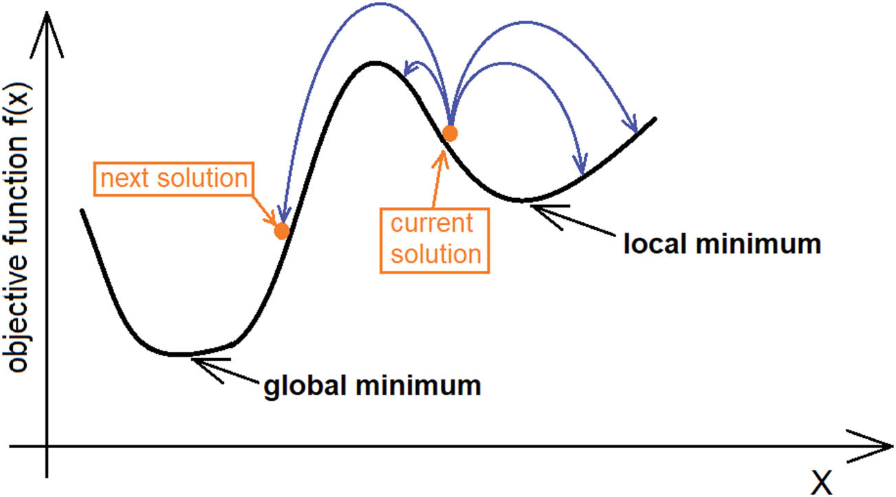
Idea of solution seeking for one-dimensional objective function.

Flowchart of the SA method.
The properties of SA algorithm, especially its ability to solve complex computational problems with local minima, led to a situation, where it is used in fields sometimes very distant from thermodynamics. The famous travelling salesman problem is frequently used as an example. Metaheuristic methods have been used to solve some optimisation problems in geodesy and surveying techniques e.g. references [24,25,26] but uses of SA in this field are limited. They include research on geodetic network design [27,28] or terrestrial laser scanning survey design [29]. Although this publication concerns an issue (coordinate transformation) of a much broader spectrum of applications, it proposes a new use for SA algorithm in the field of surveying techniques.
SA is an iterative algorithm, in which constant temperature change of a cooling liquid is replaced by incremented changes realised in subsequent iterations. Its use for solving estimation tasks requires a definition of several essential elements:
Objective function corresponding to the molecular energy level during annealing process that will be minimalised
Cooling scheme comprised assumed initial temperature and dependency defining temperature drop after each iteration
Molecule movement model corresponding to the actual temperature
Termination criteria for the iterative process. The condition can be formulated on the basis of:
final temperature (minimal),
acceptable value of the objective function,
range of molecule movement that usually corresponds to estimated model parameter changes defining the objective function.
By defining: xi – vector of the current model parameters in the ith iteration of the estimation task, f(xi) – objective function defined for the current parameters, and Δxi – change in parameter vector in the ith iteration, the SA algorithm can be presented using the following scheme:
3.1 Objective function
The objective of the algorithm is to find the global minimum. Therefore, the objective function f(xi) must provide an answer whether the current solution (xi vector) is better than the previous one and thereby if it is closer to the final solution. An equation assuming the maximal value for the end condition can also be used. In that case changing the sign brings the equation down to standard case (searching for minimum).
3.2 Cooling scheme
Temperature as a parameter of the SA algorithm stems from physical analogies. In case of optimisation tasks not related to liquid solidification it is an abstract notion. In such situation it is more important to define the function of temperature change. Various schemata are used in SA algorithms, but they always take the form of:
where T0 is the initial temperature and i is the iteration number. The fact of a tight link between current temperature and current iteration number makes it possible to replace the temperature parameter with iteration number in some solutions.
3.3 Molecule movement model
The most distinguishing feature of the SA method is the so-called molecule movement model connected with the way the new solution is obtained. It is generally defined by two elements. The first of them is the way each current (subsequent) solution is generated, which is defined by equation (6)
Δxivector is randomly generated and usually normal distribution N(0,σ) is used. Current standard deviation of this distribution σi is the function of initial value σ0 and temperature (or iteration number) in accordance to the equation:
or
If the obtained value of the objective function is lower than the current value, the new solution (xi = xi+ Δxi) is accepted unconditionally. Otherwise the obtained vector, even though it corresponds to a worse solution from the objective function’s perspective, is accepted with a determined probability p. The most advanced method – based in the thermodynamic origins of the procedure – is the application of Boltzmann distribution. The value of p is then defined by equation (10)
This method gives relatively high p values, which on the one hand provides a higher guarantee of finding the global minimum, but on the other the frequent acceptance of a worse solution considerably slows down the iteration process. A simpler solution would be to assume constant value for p – most commonly in range from 0.001 to 0.2 (like in ref. [28]). In the simplest tasks with uncomplicated spatial distribution of the objective function this element of the algorithm can be omitted, which corresponds to the original version proposed by Metropolis team [21].
3.4 Termination criteria for the iterative process
Termination of the solution seeking process may be linked to acquiring a specific temperature value, which corresponds to a certain number of carried out iterations. Another option may be reaching a satisfactory value for the objective function. In both cases it is essential to determine the critical value. It depends on the required accuracy of the solution. In particular case, SA method may be used to determine an approximate solution, which will subsequently allow for application of other methods utilising e.g. linearisation of the functional dependencies describing the given task. In this case a significantly lower number of iterations is required in order to obtain a satisfactory result.
4 Concept of a hybrid algorithm
The most important advantage of the SA algorithm is the ability to find a solution (global minimum) for a task where local minima are present. Slow cooling rate and non-zero probability of accepting worse solution are crucial in such a case. It is not without significance that the starting point of the procedure has no significant impact on the speed and possibilities of finding a solution. This means that in practice there is no need to know the approximate solution and that the starting point of the process can be assumed freely. These advantages lose their significance in the last stage of the process of finding a solution, when the current solution is the close vicinity of the sought minimum for which the objective function changes in a regular manner. It results from the fact that, in contrast to gradient methods, SA procedure uses only the value of the objective function ignoring completely the character of its distribution. For the same reason and due to the stochastic character of the solution search process itself, when using SA method such solution will always be an approximation. By proper control of termination criteria it is only possible to cause the difference between the obtained result and the global minimum to be negligible for the given task.
For the above reasons, a concept of a hybrid algorithm was born. It is comprised of two extremely distinct algorithms executed sequentially depending on the phase of solution seeking process. First the SA algorithm is used. Its ultimate goal is to find an approximation for the quaternion parameter values that will make it possible to apply the chosen gradient method in the next stage. In this case, it is the widely known least squares (LS) method using linear dependency between the coordinates of the common points and the seven parameters of 3D transformation.
Another advantage of LS lies in the consistent evaluation or result accuracy estimation – both in transformation parameters as well as its results (transformed coordinates). As the LS does not include mechanisms of dealing with gross errors, in practical applications it should be supported by the quality control routine. It can be based on LS itself [30]. It is also possible to apply another robust method such as the previously mentioned TLS [11].
5 Numerical realisation of the hybrid algorithm
Spatial coordinate transformation is described by equation (1). Assuming that the ai vector is a position vector (related to the origin of the coordinate system) the t translation vector describes the translation of the origin point of the original coordinate system. Therefore, the t vector corresponds to the position of that point in the target system. This situation is not favourable, because it is not possible to determine the approximate t components based on the coordinates of the common points – especially if the points lie within a considerable distance from the origin of the coordinate system. Consequently, in practical realisations the concept of a base point for a group of common points is utilised. In this case equation (1) takes the form (11)
where a0 and b0 vectors accordingly represent the position of the base point in the original and target system. The u = [dx, dy, dz] vector is a residual vector of the translation. The centre of gravity of the common points or a selected point belonging to this group can be used as the base point. Such approach makes it possible to easily determine all transformation parameters excluding the rotation components.
5.1 SA used for determining approximated rotation parameters
The following transformed (11) equation is used to determine approximated rotation parameters
which is used to formulate the objective function
The values sought are quaternion elements Q = [q1, q2, q3, q4] corresponding to rotation matrix R. As those elements satisfy equation (3) the search area takes on the geometric form of a four-dimensional sphere. By transforming equation (3) it is possible to eliminate one of the elements, which makes it possible to narrow the search to only three of them (e.g. q2, q3 and q4) and the fourth can be obtained through the following equation:
where q2, q3 and q4 elements must satisfy:
which reduces the search area to a three-dimensional ball. Although two values of q1 satisfy equation (3) for the three elements:
but since the rotation matrix is the same for quaternion Q1 = [q1, q2, q3, q4] and Q2 = [−q1, −q2, −q3, −q4], the search can be limited to q1 ≥ 0.
Because the sought parameters are three quaternion elements q2, q3 and q4, a temperature equivalent in the form of σ parameter is assumed, which corresponds to the sought quaternion components.
The course of the process of finding a solution is defined as the following values:
σ0 = 1.0 – initial value of the standard deviation (temperature equivalent)
β = 0.99 – standard deviation decreasing rate (cooling coefficient)
p = 0 – probability of accepting a worse solution
σend ≤ 0.1 – termination condition for SA procedure
A relatively quick standard deviation decreasing rate was assumed, which is linked to a low diversity of objective function distribution in the search area. For the same reason it was decided that the original version of the algorithm will be used, eliminating the possibility to accept an inferior solution (p = 0). Early termination (σend = 0.1) of the SA procedure is tied to the role that was assigned to this part of the algorithm. Further calculations can be realised using a different method assuming the knowledge of a suitable approximation of the final solution.
5.2 Determining the final values for the seven transformation parameters using least squares method
Knowledge of a suitable approximation of the final values of the transformation parameters opens new possibilities to choose one of many estimation methods. It is possible, for example, to take into account varied accuracy of the coordinates of the common points e.g. ref. [31]. In cases where there is a risk of gross errors occurring in the observations, one of robust estimation methods (e.g. TLS) can be applied.
As it was previously mentioned, LS method was used in the second stage of the hybrid algorithm. As the result of linearisation (11) for any of the common point i it is possible to match a segment of three correction equations. By assuming notation from ref. [8] it is possible to formulate them as equation (17)
where Vi = [Vxi,Vyi,Vzi]T is the correction vector to the coordinates.
δx – defines the unknowns vector δx = [dq1, dq2, dq3, dq4, dx, dy, dz, dλ]T – corrections to the approximated values of transformation parameters, B is a 3 × 8 coefficient matrix, created from individual coordinate derivatives (components of bi vector in equation (11)) of individual unknowns, and li = [lx, ly, lz] is the vector of residuals:
where bi determines the coordinates of the i common point in the target system, λ – current approximation of scale change coefficient, u – current approximation of translation parameters and rotation matrix R was acquired using equation (4) based on the current quaternion component values [q1,q2,q3,q4].
Having n ≥ 3 common points makes it possible to match a correction equation set in the form of
where
To calculate the vector of the unknowns it is necessary to include equation (3) corresponding to the conditional matrix (19)
Unknowns δx will be obtained by solving the system of normal equation (20)
where
The obtained unknowns are then used for correcting the previous approximation of transformation parameters xi+1 = xi + δx. Afterwards the next iteration is performed. The iteration process finishes when the vector norm of the unknowns approaches zero within the assumed distance ε:
However, one must remember that the parameter ε does not define the precision at which the unknowns are determined but only the residual effect of nonlinearity of the transformed coordinates in regard to the linear approximation of those functions.
6 Numerical test
The way the proposed algorithm operates will be illustrated on two numerical examples.
The first test object consists of eight points. Four of them (1–4) are common (reference) points and four others (5–8) are control points. Control points are not used to calculate transformation parameters. Figure 3 shows distribution of both groups of points on XOY plane.
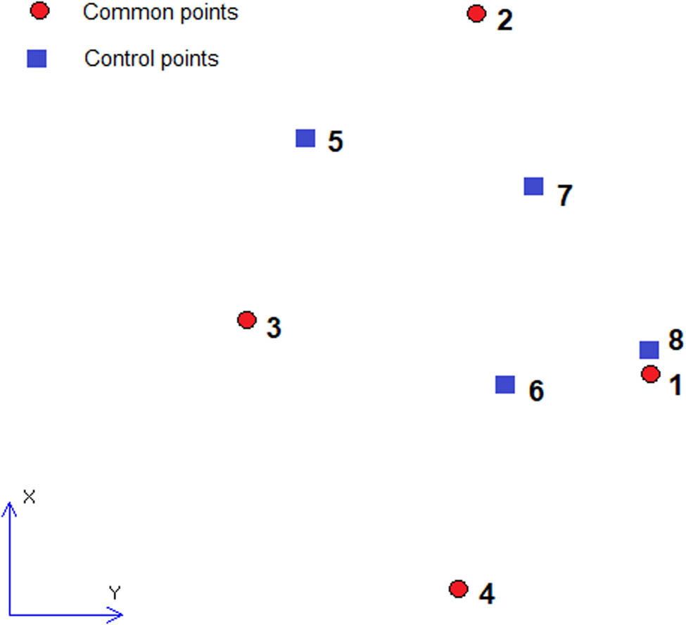
Test object 1 points placement.
Spatial coordinates of all points are presented in Table 1.
Common and control points coordinates – example 1
| System 1 [m] | System 2 [m] | |||||
|---|---|---|---|---|---|---|
| Pt | x1 | y1 | z1 | x2 | y2 | z2 |
| 1 | 21.374 | 98.615 | 112.938 | 3045.691 | 2835.122 | 39.727 |
| 2 | 134.752 | 42.840 | 0.428 | 3028.006 | 2666.808 | 37.048 |
| 3 | 36.630 | −29.441 | −22.770 | 3130.473 | 2681.592 | 105.495 |
| 4 | −48.285 | 37.710 | 86.821 | 3125.372 | 2835.167 | 93.628 |
| 5 | 94.863 | −11.198 | 86.676 | 3107.415 | 2725.879 | −9.495 |
| 6 | 15.988 | 52.207 | −48.539 | 3062.508 | 2711.755 | 152.780 |
| 7 | 79.922 | 62.372 | 132.735 | 3056.076 | 2796.734 | −19.903 |
| 8 | 25.632 | 98.525 | 21.368 | 3028.778 | 2771.709 | 103.788 |
Solution seeking process for the SA method is best illustrated using the so-called Markov chain. It consists of a sequence of states (in this case, sets of q2, q3, q4 values) corresponding to subsequent, at the time best, objective function values. Due to the stochastic character of the solution seeking process every time the procedure is stared it takes different way to approach the final solution. For that reason it is not possible to obtain two identical Markov chains by two independent starts of the SA procedure. Analysing Markov chains of SA is essential while optimising the key parameters of the procedure in the particular task.
To better illustrate how the SA algorithm is working out approximate rotation parameters the procedure was repeated three times. The Markov chains describing course of the solution seeking process for the test 1 were juxtaposed in Table 2. In the case of SA method, the total number of iterations was constant, as it is dependent on the initial value of the standard deviation value for quaternion elements – σ0, standard deviation decreasing rate – β and termination condition for the iterative process. For the values assumed here (previous chapter) it was equal to 230. The it. nr column presents the iteration numbers for which the SA procedure found the better solution.
Course of solution seeking process – example 1
| Trial no. | SA | LS | |||||
|---|---|---|---|---|---|---|---|
| it. | q2 | q3 | q4 | fobj | it. | |δx| | |
| 1 | 2 | −0.61014 | 0.29932 | 0.26327 | 3.0 × 10⁴ | 1 | 6.8 × 10³ |
| 6 | −0.06746 | 0.80368 | 0.46698 | 2.9 × 10⁴ | 2 | 1.5 × 10³ | |
| 17 | −0.33752 | 0.67297 | 0.41731 | 1.4 × 10⁴ | 3 | 2.5 × 101 | |
| 55 | −0.33125 | 0.77385 | 0.46125 | 6.5 × 10³ | 4 | 3.4 × 10⁻³ | |
| 70 | −0.42668 | 0.79239 | 0.29698 | 9.5 × 10² | |||
| 2 | 16 | −0.61091 | 0.22384 | −0.30276 | 3.5 × 10⁴ | 1 | 5.3 × 10³ |
| 17 | −0.56810 | 0.75727 | 0.15112 | 2.3 × 10³ | 2 | 3.8 × 10² | |
| 167 | −0.44612 | 0.82186 | 0.30560 | 4.3 × 10² | 3 | 1.8 × 10 | |
| 219 | −0.42750 | 0.81745 | 0.30802 | 3.4 × 10² | 4 | 1.8 × 10⁻⁴ | |
| 3 | 2 | −0.46998 | 0.42775 | −0.35724 | 2.9 × 10⁴ | 1 | 6.6 × 10³ |
| 20 | −0.55534 | 0.52513 | 0.04127 | 1.3 × 10⁴ | 2 | 1.4 × 10³ | |
| 21 | −0.26761 | 0.89556 | 0.12314 | 9.2 × 10³ | 3 | 3.5 × 101 | |
| 71 | −0.41424 | 0.86637 | 0.01111 | 6.4 × 10³ | 4 | 1.9 × 10⁻² | |
| 126 | −0.57854 | 0.67501 | 0.37977 | 4.8 × 10³ | |||
| 147 | −0.38718 | 0.79575 | 0.37317 | 2.2 × 10³ | |||
| 149 | −0.46441 | 0.85084 | 0.15977 | 1.9 × 10³ | |||
| 178 | −0.43432 | 0.81917 | 0.16067 | 1.4 × 10³ | |||
| 190 | −0.37388 | 0.84222 | 0.29749 | 1.4 × 10³ | |||
| 196 | −0.45269 | 0.78088 | 0.28901 | 6.0 × 10² | |||
Note: Values in bold are the final values of the first stage of the calculation process (SA section) or starting values for the second stage (LS section). The starting values of the LS stage can be treated as a rate of the SA stage.
The last (final) set of quaternion parameters set is marked in bold. As it can be seen, each of the three trials delivered quite similar parameters values. Differences in q2, q3 and q4 don’t exceed 10% of their values.
The unknowns vector norm of the LS first iteration (also marked in bold) can be treated as an assessment of the SA result. The final solution being the result of application of LS was always identical. Residuals on common (bold) and control points are presented in Table 3.
Residuals on common points and control points for LS solution – example 1
| Pt | Δx [m] | Δy [m] | Δz [m] |
|---|---|---|---|
| 1 | 0.0069 | −0.0043 | 0.0046 |
| 2 | −0.0054 | −0.0054 | −0.0031 |
| 3 | 0.0001 | 0.0052 | −0.0005 |
| 4 | −0.0016 | 0.0045 | −0.0010 |
| 5 | −0.0105 | −0.0055 | −0.0074 |
| 6 | 0.0036 | −0.0097 | 0.0011 |
| 7 | −0.0092 | −0.0048 | −0.0052 |
| 8 | 0.0139 | −0.0035 | 0.0065 |
Note: Values in bold are the final values of the first stage of the calculation process (SA section) or starting values for the second stage (LS section). The starting values of the LS stage can be treated as a rate of the SA stage.
Due to proper number and distribution of the first test object common points, finding transformation parameters is a well-defined and relatively easy task. To test the effectiveness of the SA algorithm in a more demanding case another test object was invented. The second test object consists of three common points and three control points. The placement of common points was selected in a very disadvantageous way. They form an elongated triangle. The layout of all the points is presented in Figure 4 and their coordinates in Table 4. All the measures in Figure 4 are in meters.
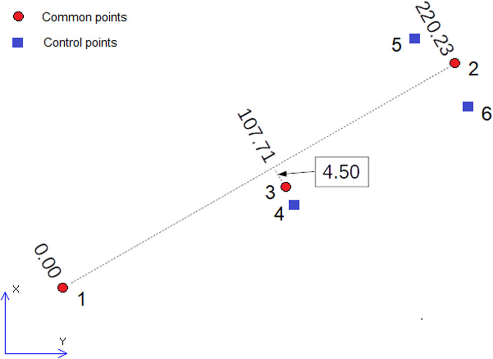
Test object 2 points placement.
Common and control points coordinates – example 2
| System 1 [m] | System 2 [m] | |||||
|---|---|---|---|---|---|---|
| Pt | x1 | y1 | z1 | x2 | y2 | z2 |
| 1 | 10.000 | 10.000 | 0.000 | 486.664 | 499.534 | 195.260 |
| 2 | 150.000 | 180.000 | 0.000 | 280.933 | 471.031 | 122.094 |
| 3 | 75.000 | 96.000 | 0.000 | 386.592 | 481.140 | 159.728 |
| 4 | 74.000 | 99.000 | 12.000 | 381.316 | 478.475 | 170.616 |
| 5 | 157.000 | 174.000 | 10.000 | 276.691 | 480.367 | 130.959 |
| 6 | 142.000 | 184.000 | 5.000 | 282.131 | 462.747 | 128.003 |
The coordinates in system 2 were obtained by rotation and translation of the established points in system 1 using equation (1), with rotation matrix R created on the basis of commonly known equations used in photogrammetry presented i.a. in reference [32] (equation (2.3)) for rotation angles ω = −167°, φ = 195°, κ = 45° respectively. A translation vector t = [500.00,500.00,200.00] was set. Coordinates in system 2 were distorted with errors generated based on normal distribution with standard deviation σxyz = ±0.02 m.
As in the previous test the procedure was repeated three times. The Markov chains describing course of the solution seeking process for test 2 were juxtaposed in Table 5.
Course of solution seeking process – example 2
| Trial no. | SA | LS | |||||
|---|---|---|---|---|---|---|---|
| it. | q2 | q3 | q4 | fobj | it. | |δx| | |
| 1 | 11 | 0.25970 | −0.87668 | 0.11922 | 2.3 × 10⁴ | 1 | 1.1 × 10⁴ |
| 33 | 0.30390 | −0.27214 | 0.69446 | 2.0 × 10⁴ | 2 | 3.1 × 10³ | |
| 42 | 0.07751 | 0.00543 | 0.95193 | 5.8 × 10³ | 3 | 9.0 × 101 | |
| 66 | −0.12058 | 0.17849 | 0.88496 | 2.1 × 10³ | 4 | 2.5 × 10⁻¹ | |
| 83 | −0.47744 | 0.31399 | 0.75136 | 1.7 × 10³ | 5 | 1.8 × 10⁻⁴ | |
| 141 | −0.43279 | 0.46618 | 0.69776 | 3.1 × 10² | |||
| 202 | −0.39075 | 0.36523 | 0.74209 | 8.5 × 101 | |||
| 2 | 3 | −0.21799 | 0.08426 | 0.96925 | 9.2 × 10³ | 1 | 8.9 × 10³ |
| 13 | −0.27265 | 0.26343 | 0.82109 | 3.5 × 10² | 2 | 1.4 × 10³ | |
| 131 | −0.08587 | −0.26250 | 0.90688 | 1.4 × 10² | 3 | 6.7 × 101 | |
| 4 | 1.1 × 10⁻¹ | ||||||
| 5 | 8.0 × 10⁻⁵ | ||||||
| 3 | 3 | −0.39293 | 0.06396 | 0.57403 | 1.9 × 10⁴ | 1 | 1.1 × 10⁴ |
| 8 | −0.64238 | 0.73165 | 0.13101 | 2.9 × 10³ | 2 | 2.7 × 10³ | |
| 22 | −0.46757 | 0.41313 | 0.61078 | 2.2 × 10³ | 3 | 1.4 × 10² | |
| 57 | −0.35814 | 0.39209 | 0.75010 | 6.5 × 101 | 4 | 3.2 × 10⁻¹ | |
| 5 | 2.0 × 10⁻⁴ | ||||||
Note: Values in bold are the final values of the first stage of the calculation process (SA section) or starting values for the second stage (LS section). The starting values of the LS stage can be treated as a rate of the SA stage.
Residuals on common and control points are presented in Table 6.
Residuals on common and control points for LS solution – example 2
| Pt | Δx [m] | Δy [m] | Δz [m] |
|---|---|---|---|
| 1 | 0.0052 | 0.0012 | 0.0018 |
| 2 | 0.0050 | 0.0007 | 0.0018 |
| 3 | −0.0102 | −0.0019 | −0.0036 |
| 4 | −0.0258 | −0.0669 | −0.0051 |
| 5 | −0.0350 | −0.0535 | 0.1078 |
| 6 | 0.0188 | −0.0404 | −0.0588 |
Note: Values in bold are the final values of the first stage of the calculation process (SA section) or starting values for the second stage (LS section). The starting values of the LS stage can be treated as a rate of the SA stage.
Despite the significant disadvantage resulting from the placement of common points the SA procedure was able to deliver angular transformation parameters that were good enough, so that the subsequently introduced LS procedure was able to provide the exact solution after a few iterations. The Markov chains (columns q2, q3 and q4) presented in Table 5 point to a high diversity in the way the solution was reached. Relatively big differences present themselves in the final quaternion component values. It is especially true of q3 component. The previous test and other experiments carried out by the author that are not presented in this paper indicate that these discrepancies are closely linked to point set geometry and can be reduced to small extent by increasing the precision of the SA method (e.g. by slowing down the standard deviation decreasing rate or delaying the termination of solution seeking process by decreasing value of σend).
Disadvantageous geometry of the common points is also responsible for large residuals on the control points shown in Table 6.
It is worth remembering that even though all tests presented in Table 5 were successful, due to the random nature of the SA procedure itself one cannot eliminate the possibility of a failure, which will be understood as obtaining a solution distant from the final one. The probability of a failure increases the more the SA parameters are optimised for processing speed. In such case an attempt to continue the process using LS will lead to a situation, where two subsequent iterations i and i + 1 will produce an inequality |δxi+1| ≥ |δxi|, which will be interpreted as an error and will terminate the LS iteration process. If SA parameters have been selected correctly, a repeated attempt to solve the task is the best countermeasure.
7 Conclusions
The performed computational tests confirmed the predicted effectiveness of the SA procedure in solving a fundamental 3D transformation problem, namely to determine approximate values of parameters defining the change in orientation. While the first numerical test used to check and demonstrate the algorithm using four regularly distributed common points can be considered as easy, the second one utilised an extremely disadvantageous placement of three common points. Poor geometry of common points caused the distribution of the objective function in the space of the sought parameters to be less clear. In result, quaternion elements being rotation parameters obtained as a result of SA procedure in the second test were much more differentiated among subsequent trials.
It should be noted that the length of the Markov chains presented in Tables 2 and 5 did not exceed 10 nodes for 230 iterations. Such nature of the process results from the used parameters which caused the SA procedure to progress relatively quickly (β = 0.99) and finish relatively early (σend = 0.1). The selection of parameters proved sufficient even in the case of unfavourable geometry. The unfavourable geometry of the common points in test 2 also caused that, on average, one more iteration of LS were needed to obtain the final solution.
The author is aware of the shortcomings of the LS method, of which the most often referenced one is insufficient robustness in case of presence of gross errors. That is why its application in the described algorithm is of demonstrative value only. Nothing prevents software used for real 3D tasks from utilising a robust estimation method e.g. TLS.
Due to the high probable diversity of cases as well as high dependency of the course of the SA procedure and the precision of the delivered results on its control parameters, one should provide an advanced user the possibility to modify these parameters in order to optimise the course of calculations for specific cases.
In the case of a numerous common points their number can be limited in order to accelerate the SA algorithm operation process (only approximated values are needed).
Parameters of SA procedure were optimised for potentially least optimal case and were assumed as constant. It seems that in case of more advantageous distribution of common points and larger number of them it is possible to accelerate the solution seeking process. Formulating rules for customisation of SA parameters with regard to the task’s characteristic needs requires further research.
References
[1] Helmert FR. Die Europaische Langengradmessung in 52 Grad Breite von Greenwich bis Warchau. I. Heft. Veroff. des Konigl. Berlin: Preussischen Geodätischen Instituts und Centralbureaus der Int. Erdmessung; 1893. p. 47–50. (in German).Suche in Google Scholar
[2] Teunissen PJ. The non-linear 2D symmetric Helmert transformation: an exact non-linear least-squares solution. B Geo. 1988;62(1):1–16.10.1007/BF02519322Suche in Google Scholar
[3] Watson GA. Computing Helmert transformations. J Comput Appl Math. 2006;197(2):387–94. 10.1016/j.cam.2005.06.047.Suche in Google Scholar
[4] Grafarend EW, Awange JL. Nonlinear analysis of the three-dimensional datum transformation [conformal group ℂ 7 (3)]. J Geodesy. 2003;77(1–2):66–76. 10.1007/s00190-002-0299-9.Suche in Google Scholar
[5] Păun CD, Oniga VO, Dragomir PI. Three-dimensional transformation of coordinate systems using nonlinear analysis – Procrustes algorithm. Int J Eng Sci Res Technol. 2017;6(2):355–63. 10.5281/zenodo.291839.Suche in Google Scholar
[6] Zeng H. Analytical algorithm of weighted 3D datum transformation using the constraint of orthonormal matrix. Earth Planets Space. 2015;67(1):105. 10.1186/s40623-015-0263-6.Suche in Google Scholar
[7] Hanson AJ. Extensions and Exact Solutions to the Quaternion-Based RMSD Problem. arXiv preprint, 2018, arXiv:1804.03528.Suche in Google Scholar
[8] Zeng H, Yi Q. Quaternion-based iterative solution of three-dimensional coordinate transformation problem. JCP. 2011;6(7):1361–8.10.4304/jcp.6.7.1361-1368Suche in Google Scholar
[9] Paláncz B, Awange JL, Völgyesi L. Pareto optimality solution of the Gauss–Helmert model. Acta Geod Geophys. 2013;48(3):293–304. 10.1007/s40328-013-0027-3.Suche in Google Scholar
[10] El-Habiby MM, Gao Y, Sideris MG. Comparison and analysis of non-linear least squares methods for 3-D coordinates transformation. Surv Rev. 2009;41(311):26–43. 10.1179/003962608X389988.Suche in Google Scholar
[11] Akyilmaz O. Total least-squares solution of coordinate transformation. Surv Rev. 2007;39(303):68–80. 10.1179/003962607X165005.Suche in Google Scholar
[12] Hamilton WR. On quaternions; or a new system of imaginaries in algebra. Philos Mag. 1844;25:489–95.Suche in Google Scholar
[13] Rodrigues O. Des lois géométriques qui régissent les déplacements d’un système solide dans l’espace, et de la variation des coordonnées provenant de ces déplacements considérés indépendamment des causes qui peuvent les produire. J Math Pure Appl. 1840;1re série, tome 5:380–440. (in French).Suche in Google Scholar
[14] Altmann SL. Hamilton Rodrigues and the quaternion scandal. Math Mag. 1989;62(5):291–308. 10.1080/0025570X.1989.11977459.Suche in Google Scholar
[15] Hanson AJ. Visualizing Quaternions. Morgan-Kaufmann/Elsevier; 2006.10.1145/1198555.1198701Suche in Google Scholar
[16] Mukundan R. Quaternions: from classical mechanics to computer graphics, and beyond. Proceedings of the 7th Asian Technology conference in Mathematics. 2002. p. 97–105.Suche in Google Scholar
[17] Arribas M, Elipe A, Palacios M. Quaternions and the rotation of a rigid body. Celest Mech Dyn Astr. 2006;96(3–4):239–51. 10.1007/s10569-006-9037-6.Suche in Google Scholar
[18] Shuster MD, Natanson GA. Quaternion computation from a geometric point of view. J Astronaut Sci. 1993;41(4):545–56.Suche in Google Scholar
[19] Coutsias EA, Seok C, Dill KA. Using quaternions to calculate RMSD. J Comput Chem. 2004;25(15):1849–57. 10.1002/jcc.20110.Suche in Google Scholar PubMed
[20] Popov P, Grudinin S. Rapid determination of RMSDs corresponding to macromolecular rigid body motions. J Comput Chem. 2014;35(12):950–6. 10.1002/jcc.23569.Suche in Google Scholar PubMed
[21] Metropolis N, Rosenbluth AW, Rosenbluth MN, Teller AH, Teller E. Equation of state calculations by fast computing machines. J Chem Phys. 1953;21(6):1087–92. 10.1063/1.1699114.Suche in Google Scholar
[22] Kirkpatrick S, Gelatt Jr CD, Vecchi MP. Optimization by simulated annealing. Science. 1983;220(4598):671–80. 10.1126/science.220.4598.671.Suche in Google Scholar PubMed
[23] van Laarhoven PJM, Aarts EHL. Simulated annealing: Theory and applications. Dordrecht, The Netherlands: Reidel; 1987.10.1007/978-94-015-7744-1Suche in Google Scholar
[24] Yetkin M. Metaheuristic optimisation approach for designing reliable and robust geodetic networks. Surv Rev. 2013;45(329):136–40.10.1080/17522706.2013.12287495Suche in Google Scholar
[25] Yetkin M, Berber M. Implementation of robust estimation in GPS networks using the artificial bee colony algorithm. Earth Sci Inf. 2014;7(1):39–46. 10.1007/s12145-013-0131-5.Suche in Google Scholar
[26] Yetkin M. Application of robust estimation in geodesy using the harmony search algorithm. J Spat Sci. 2018;63(1):63–73. 10.1080/14498596.2017.1341856.Suche in Google Scholar
[27] Berné JL, Baselga S. First-order design of geodetic networks using the simulated annealing method. J Geodesy. 2004;78(1–2):47–54. 10.1007/s00190-003-0365-y.Suche in Google Scholar
[28] Baselga S. Second order design of geodetic networks by the simulated annealing method. J Surv Eng. 2011;137(4):167–73. 10.1061/(ASCE)SU.1943-5428.0000053.Suche in Google Scholar
[29] Jia F, Lichti D. Comparison a of simulated annealing, genetic algorithm and particle swarm optimization in optimal first-order design of indoor TLS networks. ISPRS Ann Photogramm Remote Sens Spat Inf Sci. 2017;IV-2/W4:75–82. 10.5194/isprs-annals-IV-2-W4-75-2017.Suche in Google Scholar
[30] Prószyński W. Measuring the robustness potential of the least-squares estimation: geodetic illustration. J Geodesy. 1997;71(10):652–9. 10.1007/s001900050132.Suche in Google Scholar
[31] Kwaśniak M, Prószyński W. The stochastic approach to coordinate transformation for the needs of engineering surveys. Geodezja i Kartogr. 1998;47(3–4):267–80.Suche in Google Scholar
[32] Schut GH. An Introduction to Analytical Strip-Triangulation with a Fortran Progam. Vol. 1. National Research Council of Canada Report, No. NRC; 1973. p. 3148.Suche in Google Scholar
© 2020 Waldemar Odziemczyk, published by De Gruyter
This work is licensed under the Creative Commons Attribution 4.0 International License.
Artikel in diesem Heft
- Regular Articles
- The simulation approach to the interpretation of archival aerial photographs
- The application of137Cs and210Pbexmethods in soil erosion research of Titel loess plateau, Vojvodina, Northern Serbia
- Provenance and tectonic significance of the Zhongwunongshan Group from the Zhongwunongshan Structural Belt in China: insights from zircon geochronology
- Analysis, Assessment and Early Warning of Mudflow Disasters along the Shigatse Section of the China–Nepal Highway
- Sedimentary succession and recognition marks of lacustrine gravel beach-bars, a case study from the Qinghai Lake, China
- Predicting small water courses’ physico-chemical status from watershed characteristics with two multivariate statistical methods
- An Overview of the Carbonatites from the Indian Subcontinent
- A new statistical approach to the geochemical systematics of Italian alkaline igneous rocks
- The significance of karst areas in European national parks and geoparks
- Geochronology, trace elements and Hf isotopic geochemistry of zircons from Swat orthogneisses, Northern Pakistan
- Regional-scale drought monitor using synthesized index based on remote sensing in northeast China
- Application of combined electrical resistivity tomography and seismic reflection method to explore hidden active faults in Pingwu, Sichuan, China
- Impact of interpolation techniques on the accuracy of large-scale digital elevation model
- Natural and human-induced factors controlling the phreatic groundwater geochemistry of the Longgang River basin, South China
- Land use/land cover assessment as related to soil and irrigation water salinity over an oasis in arid environment
- Effect of tillage, slope, and rainfall on soil surface microtopography quantified by geostatistical and fractal indices during sheet erosion
- Validation of the number of tie vectors in post-processing using the method of frequency in a centric cube
- An integrated petrophysical-based wedge modeling and thin bed AVO analysis for improved reservoir characterization of Zhujiang Formation, Huizhou sub-basin, China: A case study
- A grain size auto-classification of Baikouquan Formation, Mahu Depression, Junggar Basin, China
- Dynamics of mid-channel bars in the Middle Vistula River in response to ferry crossing abutment construction
- Estimation of permeability and saturation based on imaginary component of complex resistivity spectra: A laboratory study
- Distribution characteristics of typical geological relics in the Western Sichuan Plateau
- Inconsistency distribution patterns of different remote sensing land-cover data from the perspective of ecological zoning
- A new methodological approach (QEMSCAN®) in the mineralogical study of Polish loess: Guidelines for further research
- Displacement and deformation study of engineering structures with the use of modern laser technologies
- Virtual resolution enhancement: A new enhancement tool for seismic data
- Aeromagnetic mapping of fault architecture along Lagos–Ore axis, southwestern Nigeria
- Deformation and failure mechanism of full seam chamber with extra-large section and its control technology
- Plastic failure zone characteristics and stability control technology of roadway in the fault area under non-uniformly high geostress: A case study from Yuandian Coal Mine in Northern Anhui Province, China
- Comparison of swarm intelligence algorithms for optimized band selection of hyperspectral remote sensing image
- Soil carbon stock and nutrient characteristics of Senna siamea grove in the semi-deciduous forest zone of Ghana
- Carbonatites from the Southern Brazilian platform: I
- Seismicity, focal mechanism, and stress tensor analysis of the Simav region, western Turkey
- Application of simulated annealing algorithm for 3D coordinate transformation problem solution
- Application of the terrestrial laser scanner in the monitoring of earth structures
- The Cretaceous igneous rocks in southeastern Guangxi and their implication for tectonic environment in southwestern South China Block
- Pore-scale gas–water flow in rock: Visualization experiment and simulation
- Assessment of surface parameters of VDW foundation piles using geodetic measurement techniques
- Spatial distribution and risk assessment of toxic metals in agricultural soils from endemic nasopharyngeal carcinoma region in South China
- An ABC-optimized fuzzy ELECTRE approach for assessing petroleum potential at the petroleum system level
- Microscopic mechanism of sandstone hydration in Yungang Grottoes, China
- Importance of traditional landscapes in Slovenia for conservation of endangered butterfly
- Landscape pattern and economic factors’ effect on prediction accuracy of cellular automata-Markov chain model on county scale
- The influence of river training on the location of erosion and accumulation zones (Kłodzko County, South West Poland)
- Multi-temporal survey of diaphragm wall with terrestrial laser scanning method
- Functionality and reliability of horizontal control net (Poland)
- Strata behavior and control strategy of backfilling collaborate with caving fully-mechanized mining
- The use of classical methods and neural networks in deformation studies of hydrotechnical objects
- Ice-crevasse sedimentation in the eastern part of the Głubczyce Plateau (S Poland) during the final stage of the Drenthian Glaciation
- Structure of end moraines and dynamics of the recession phase of the Warta Stadial ice sheet, Kłodawa Upland, Central Poland
- Mineralogy, mineral chemistry and thermobarometry of post-mineralization dykes of the Sungun Cu–Mo porphyry deposit (Northwest Iran)
- Main problems of the research on the Palaeolithic of Halych-Dnister region (Ukraine)
- Application of isometric transformation and robust estimation to compare the measurement results of steel pipe spools
- Hybrid machine learning hydrological model for flood forecast purpose
- Rainfall thresholds of shallow landslides in Wuyuan County of Jiangxi Province, China
- Dynamic simulation for the process of mining subsidence based on cellular automata model
- Developing large-scale international ecological networks based on least-cost path analysis – a case study of Altai mountains
- Seismic characteristics of polygonal fault systems in the Great South Basin, New Zealand
- New approach of clustering of late Pleni-Weichselian loess deposits (L1LL1) in Poland
- Implementation of virtual reference points in registering scanning images of tall structures
- Constraints of nonseismic geophysical data on the deep geological structure of the Benxi iron-ore district, Liaoning, China
- Mechanical analysis of basic roof fracture mechanism and feature in coal mining with partial gangue backfilling
- The violent ground motion before the Jiuzhaigou earthquake Ms7.0
- Landslide site delineation from geometric signatures derived with the Hilbert–Huang transform for cases in Southern Taiwan
- Hydrological process simulation in Manas River Basin using CMADS
- LA-ICP-MS U–Pb ages of detrital zircons from Middle Jurassic sedimentary rocks in southwestern Fujian: Sedimentary provenance and its geological significance
- Analysis of pore throat characteristics of tight sandstone reservoirs
- Effects of igneous intrusions on source rock in the early diagenetic stage: A case study on Beipiao Formation in Jinyang Basin, Northeast China
- Applying floodplain geomorphology to flood management (The Lower Vistula River upstream from Plock, Poland)
- Effect of photogrammetric RPAS flight parameters on plani-altimetric accuracy of DTM
- Morphodynamic conditions of heavy metal concentration in deposits of the Vistula River valley near Kępa Gostecka (central Poland)
- Accuracy and functional assessment of an original low-cost fibre-based inclinometer designed for structural monitoring
- The impacts of diagenetic facies on reservoir quality in tight sandstones
- Application of electrical resistivity imaging to detection of hidden geological structures in a single roadway
- Comparison between electrical resistivity tomography and tunnel seismic prediction 303 methods for detecting the water zone ahead of the tunnel face: A case study
- The genesis model of carbonate cementation in the tight oil reservoir: A case of Chang 6 oil layers of the Upper Triassic Yanchang Formation in the western Jiyuan area, Ordos Basin, China
- Disintegration characteristics in granite residual soil and their relationship with the collapsing gully in South China
- Analysis of surface deformation and driving forces in Lanzhou
- Geochemical characteristics of produced water from coalbed methane wells and its influence on productivity in Laochang Coalfield, China
- A combination of genetic inversion and seismic frequency attributes to delineate reservoir targets in offshore northern Orange Basin, South Africa
- Explore the application of high-resolution nighttime light remote sensing images in nighttime marine ship detection: A case study of LJ1-01 data
- DTM-based analysis of the spatial distribution of topolineaments
- Spatiotemporal variation and climatic response of water level of major lakes in China, Mongolia, and Russia
- The Cretaceous stratigraphy, Songliao Basin, Northeast China: Constrains from drillings and geophysics
- Canal of St. Bartholomew in Seča/Sezza: Social construction of the seascape
- A modelling resin material and its application in rock-failure study: Samples with two 3D internal fracture surfaces
- Utilization of marble piece wastes as base materials
- Slope stability evaluation using backpropagation neural networks and multivariate adaptive regression splines
- Rigidity of “Warsaw clay” from the Poznań Formation determined by in situ tests
- Numerical simulation for the effects of waves and grain size on deltaic processes and morphologies
- Impact of tourism activities on water pollution in the West Lake Basin (Hangzhou, China)
- Fracture characteristics from outcrops and its meaning to gas accumulation in the Jiyuan Basin, Henan Province, China
- Impact evaluation and driving type identification of human factors on rural human settlement environment: Taking Gansu Province, China as an example
- Identification of the spatial distributions, pollution levels, sources, and health risk of heavy metals in surface dusts from Korla, NW China
- Petrography and geochemistry of clastic sedimentary rocks as evidence for the provenance of the Jurassic stratum in the Daqingshan area
- Super-resolution reconstruction of a digital elevation model based on a deep residual network
- Seismic prediction of lithofacies heterogeneity in paleogene hetaoyuan shale play, Biyang depression, China
- Cultural landscape of the Gorica Hills in the nineteenth century: Franciscean land cadastre reports as the source for clarification of the classification of cultivable land types
- Analysis and prediction of LUCC change in Huang-Huai-Hai river basin
- Hydrochemical differences between river water and groundwater in Suzhou, Northern Anhui Province, China
- The relationship between heat flow and seismicity in global tectonically active zones
- Modeling of Landslide susceptibility in a part of Abay Basin, northwestern Ethiopia
- M-GAM method in function of tourism potential assessment: Case study of the Sokobanja basin in eastern Serbia
- Dehydration and stabilization of unconsolidated laminated lake sediments using gypsum for the preparation of thin sections
- Agriculture and land use in the North of Russia: Case study of Karelia and Yakutia
- Textural characteristics, mode of transportation and depositional environment of the Cretaceous sandstone in the Bredasdorp Basin, off the south coast of South Africa: Evidence from grain size analysis
- One-dimensional constrained inversion study of TEM and application in coal goafs’ detection
- The spatial distribution of retail outlets in Urumqi: The application of points of interest
- Aptian–Albian deposits of the Ait Ourir basin (High Atlas, Morocco): New additional data on their paleoenvironment, sedimentology, and palaeogeography
- Traditional agricultural landscapes in Uskopaljska valley (Bosnia and Herzegovina)
- A detection method for reservoir waterbodies vector data based on EGADS
- Modelling and mapping of the COVID-19 trajectory and pandemic paths at global scale: A geographer’s perspective
- Effect of organic maturity on shale gas genesis and pores development: A case study on marine shale in the upper Yangtze region, South China
- Gravel roundness quantitative analysis for sedimentary microfacies of fan delta deposition, Baikouquan Formation, Mahu Depression, Northwestern China
- Features of terraces and the incision rate along the lower reaches of the Yarlung Zangbo River east of Namche Barwa: Constraints on tectonic uplift
- Application of laser scanning technology for structure gauge measurement
- Calibration of the depth invariant algorithm to monitor the tidal action of Rabigh City at the Red Sea Coast, Saudi Arabia
- Evolution of the Bystrzyca River valley during Middle Pleistocene Interglacial (Sudetic Foreland, south-western Poland)
- A 3D numerical analysis of the compaction effects on the behavior of panel-type MSE walls
- Landscape dynamics at borderlands: analysing land use changes from Southern Slovenia
- Effects of oil viscosity on waterflooding: A case study of high water-cut sandstone oilfield in Kazakhstan
- Special Issue: Alkaline-Carbonatitic magmatism
- Carbonatites from the southern Brazilian Platform: A review. II: Isotopic evidences
- Review Article
- Technology and innovation: Changing concept of rural tourism – A systematic review