Application of isometric transformation and robust estimation to compare the measurement results of steel pipe spools

1 Introduction

One of the tasks carried out by survey engineers working in the offshore oil and gas industry is the measurement of pipe spools [14,15,16,17]. Spools can be defined as prefabricated components consisting of connected, welded steel elements (such as pipes, flanges and elbows) of various shapes and sizes (Figure 1). Components prepared in that manner are used during the renovation and modernization of industrial installations located on offshore oil platforms. Due to the difficulty of maintenance work in high seas, fragments of installations which are to be replaced are prepared in factories onshore and then transported to the final assembly place. Limitations concerning the scope of potentially hazardous works carried out on an oil rig (e.g., welding, cutting or grinding) make a bolted flange virtually the only possible method of connecting a prefabricated pipe spool to the existing installations.

Figure 1

Schematic view of example spool.

This method of assembly does not pose a risk associated with explosion and does not require stopping the work of the entire platform, which would generate huge costs. For this reason, prefabricated spools are most often ended with flanges.

The process of building a prefabricated pipe spool involves assembling previously prepared basic elements (fragments of pipes, elbows and flanges) into one unit. Due to the need to precisely fit the spool to be built into the existing installations at the place of the final assembly, shape measurement is an important part of the whole process. The purpose of the measurement is to ensure geometrical compatibility of the spool to be constructed with the design. The size of the finished spools, reaching sometimes even few dozens of meters, and the expected sub-millimeter accuracy of the assembly necessitate the use of the traditional methods of surveying for this purpose – i.e., maximum precision total stations along with the appropriate sets of prisms.

At the final assembly site on the oil rig, a local reference system is most often established. Based on this system, measurements of existing installations are carried out, which later form the basis for the development of the design project. In this system, designers determine both the position and other parameters of the prepared spool. The design project contains information about the location and size of the key elements of the spool and a detailed description of the direction and rotation of the flanges at the place of the final assembly.

After the first (initial) arrangement of all basic elements, the process of building a prefabricated spool is mainly accomplished through repetition of the following steps: measurement, comparison of the geometry of the spool to be built with the design along with specifying suggested corrections and implementations of the changes in the spool being built. These steps are repeated until the desired compliance with the design project is achieved. For obvious reasons, the measurement is taken in the local reference system, available at the construction site, not in the system related to the place of the final assembly in which the design project is made. This system can be defined by a local set of control points established for the needs of construction or, in the case of smaller spools, which can be measured from a single setup, and it can be a random coordinate system related to the instrument at the time of measurement.

The results of the measurement of angular and linear values are recalculated to obtain a set of coordinates XYZ of crucial points of the spool, such as intersection points of axes of pipes (elbows) and a set of parameters describing the flange. During construction, the entire spool is arranged in a manner convenient for assembly (Figure 2), which means that its position relative to the local reference system is completely different from the position relative to the reference system at the place of final assembly.

Figure 2

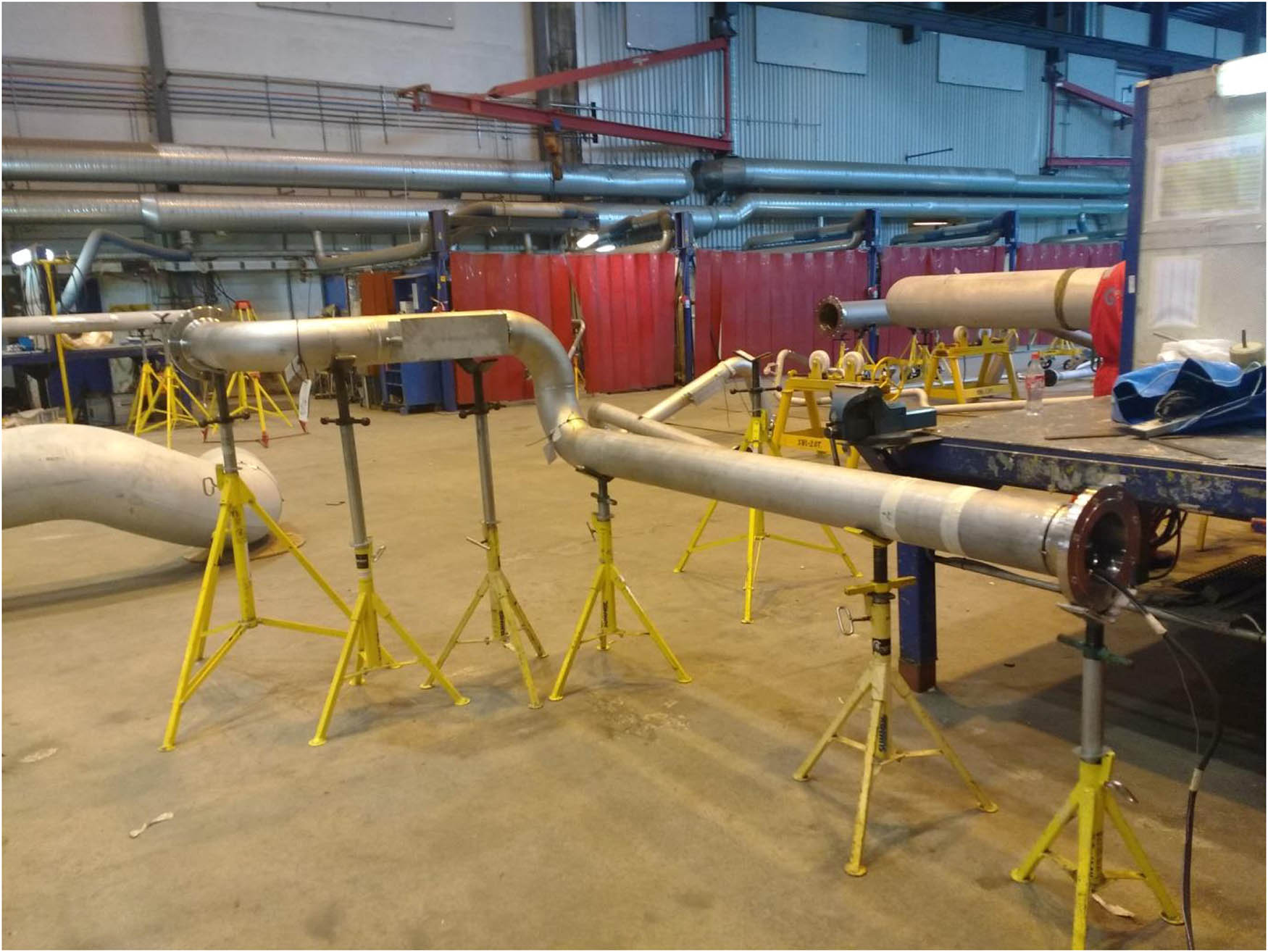
Pipe spools under construction.

The key moment of the whole process is the comparison of the measurement results of the pipe spool being constructed with the design. Its purpose is to determine the differences between what has been built and the design and thus suggest changes that should be made in the geometry of the spool. Due to the efficiency of construction works, changes should be suggested, so that their number is as small as possible; however, the size of the changes does not necessarily have to be small. To illustrate, if it is only possible, it is better to suggest one big change rather than a few smaller ones, even if both sets of proposed corrections ultimately lead to a similar result.

At present, survey engineers performing measurements in factories use relatively simple methods of comparison. Both the design and the pre-processed measurement results of the spool being built are entered into a CAD program or other specialized software. Then with the use of rotations and translations, the measurement results are brought to a position as close as possible to the design. Differences between the design and measurement results are determined by comparing the obtained coordinates and flange parameters. The rotations and translations themselves can be defined in a variety of ways, often quite sophisticated, but they are always these two elementary activities. The sequence of implemented translations and rotations depends on the experience and intuition of the survey engineer, but the aim is to compare the spools, so that the number of differences is minimal. Such a method of comparison is effective and usually gives satisfactory results but the whole process can be time-consuming. The time necessary to perform the comparison depends on both the complexity of the spool and the survey engineer’s experience.

Additionally, during the construction of one spool, the entire procedure is repeated many times, which means that the automation of the comparison process could contribute to the efficiency of the survey engineer’s work and increase the quality of the work.

2 Research problem

An important research problem is the development of a method that allows accelerating and increasing the reliability of comparison between two pipe spools by automating the computational part of the process. It is extremely important in such a complex measurement and assembly conditions. Therefore, a method for automating the task of comparing spools with the use of isometric transformation and robust estimation has been proposed to replace traditional computational methods based on repeated translations and rotations of the spool model. Both isometric transformation and robust estimation methods are known and widely used in various tasks in the field of surveying engineering (e.g., [1,2,5,11,12,13]); however, the authors did not find scientific publications or practical implementation of the comparison process of spools using both methods. Isometric transformation (without changing the scale) allows recalculating a set of points with XYZ coordinates from the input to the output coordinate system by combining translations and rotations. Robust estimation is a set of methods for the solution of overdetermined system of equations in which the influence of outliers on the final result of the solution is minimal. It is often used, for example, to search for mistakes in surveying observations.

Some proposals for automating that process have already been presented in earlier articles (e.g., [14,15]); however, they are mainly related to using laser scanner data, whereas it is the total station measurement methods usually used in everyday practice. Such a method fits in wider trend of automating measurement processes [9].

3 Isometric transformation and robust estimation

The general isometric transformation model assumes that on the basis of two coordinate sets of control points:

• {(x_k, y_k, z_k): k = 1, 2,…,s} subset of input coordinates,

• {(X_k, Y_k, Z_k): k = 1, 2,…,s} subset of output coordinates,

a functional model of isometric transformation is determined [3]:

where:

• x = [x, y, z]^T – vector of input coordinates,

• X = [X, Y, Z]^T – vector of output coordinates,

• T = [T_X, T_Y, T_Z]^T – translation vector,

• R – rotation matrix which is a function of rotation angles α, β, γ around coordinates system axes:

where:

Such a defined transformation is the composition of rotations and translations without changing the scale of the entire system. The estimation of parameters is based on the sets of control points and is solved using the least squares method (LSM):

where:

• V_k – vector of residuals,

• φ(α, β, γ, T_X, T_Y, T_Z) – minimized function.

The above task is usually solved by the standard Gauss–Newton method.

Robust estimation can be implemented in various ways. A common method is the use of weight function which modifies the weight matrix during the iterative solving of an equation system in such a way that the weights of observations that appear to be outliers are gradually reduced. Examples of weight functions described in literature are, e.g., Huber method [4], Danish method [10], Method of Growing Rigor [8], or Choice Rule of Alternative method [7]. The selection of the best weight function for a given task depends on various criteria, e.g. [8]. However, as shown in [6], a more appropriate, theoretically justified method of robust estimation is the application of the rule which is a modification of least module method:

The least module method, due to discontinuity of second derivatives, is impossible to be solved by Newtonian methods. In practice using regularized objective function is suggested. It leads to the following equation:

where c denotes numerical parameter, larger than zero, thus (V² + c)^1/2 ≥ |V|, if c > 0.

Replacement of the absolute value by square root with parameter c allows using classical Newtonian methods to minimize the objective function. This parameter should be chosen empirically depending on a given task. In practical implementation for the problem described in this article, value c was assumed as:

where μ denotes a priori standard deviation of single coordinate.

The development of the minimum conditions leads to normal equations in the form analogous to LSM but with a diagonal weight matrix, whose elements are a function of corrections. Since the correction depends on the value of unknowns, the resulting equation is the basis for the iterative process. The weight matrix is modified during each iteration.

4 Standard description of a flange

Flanges are very important elements of each spool. With the help of flanges, the entire spool is joined with the existing installations at the place of the final assembly [19]. The shape and size of the flange itself is determined at the stage of its production by metrological methods, the accuracy of which significantly surpasses surveying techniques. Therefore, the measurement of their dimensions at the stage of constructing the spool is only of control importance. It is crucial, from the point of view of the survey engineer taking the measurement of the prefabricated spool, to determine how the flange was attached to the prefabricated structure.

Both the design engineers and people who assemble the pipe spools in the factory use a certain system of determining the position and direction of the flange in relation to the target coordinate system. The standard parameters describing the flange are:

1. XYZ coordinates of tie point (TP) coordinates, which determine the position of the flange and the angles describing the direction in which the flange’s face is directed and how it is rotated. A TP denotes the point at the intersection of the flange’s face and the main axis of the flange symmetry (Figure 3).

2. Angles defining the direction:

1. Horizontal bearing (B_Hz): horizontal deflection which is in fact the azimuth angle of the face (Figure 3a).

2. Vertical bearing (B_V): vertical deflection determining the angle value between the horizontal plane and the normal vector of the face (Figure 3b).

1. The angle which determines the position of the bolt holes. The flange is always constructed in such a way that the holes are evenly distributed over the entire circumference of the flange’s face.

The position of the holes is determined by the angle of rotation (C_B) of the flange around the main axis of symmetry. It is defined as the angle between the lines P and M. The straight line P can be defined in two ways: as the intersection of the flange’s face with the vertical plane containing the main symmetry axis S (Figure 4a) or as the intersection of the horizontal plane containing the TP with the flange’s face (Figure 4b).

Figure 3

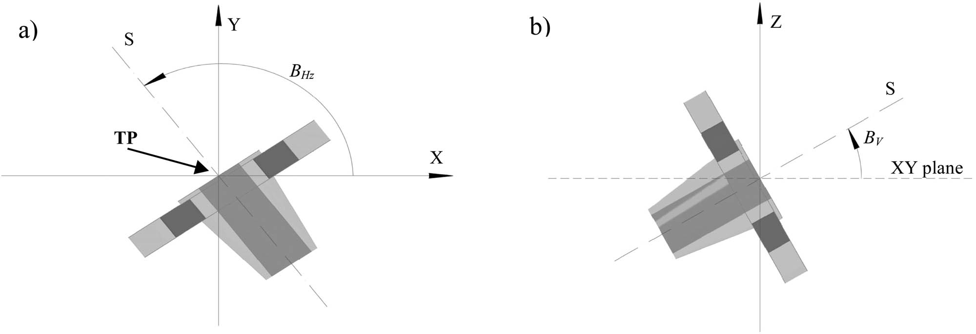
(a) Horizontal bearing B_Hz, (b) vertical bearing B_V; S – main axis of the flange symmetry; TP – tie point.

Figure 4

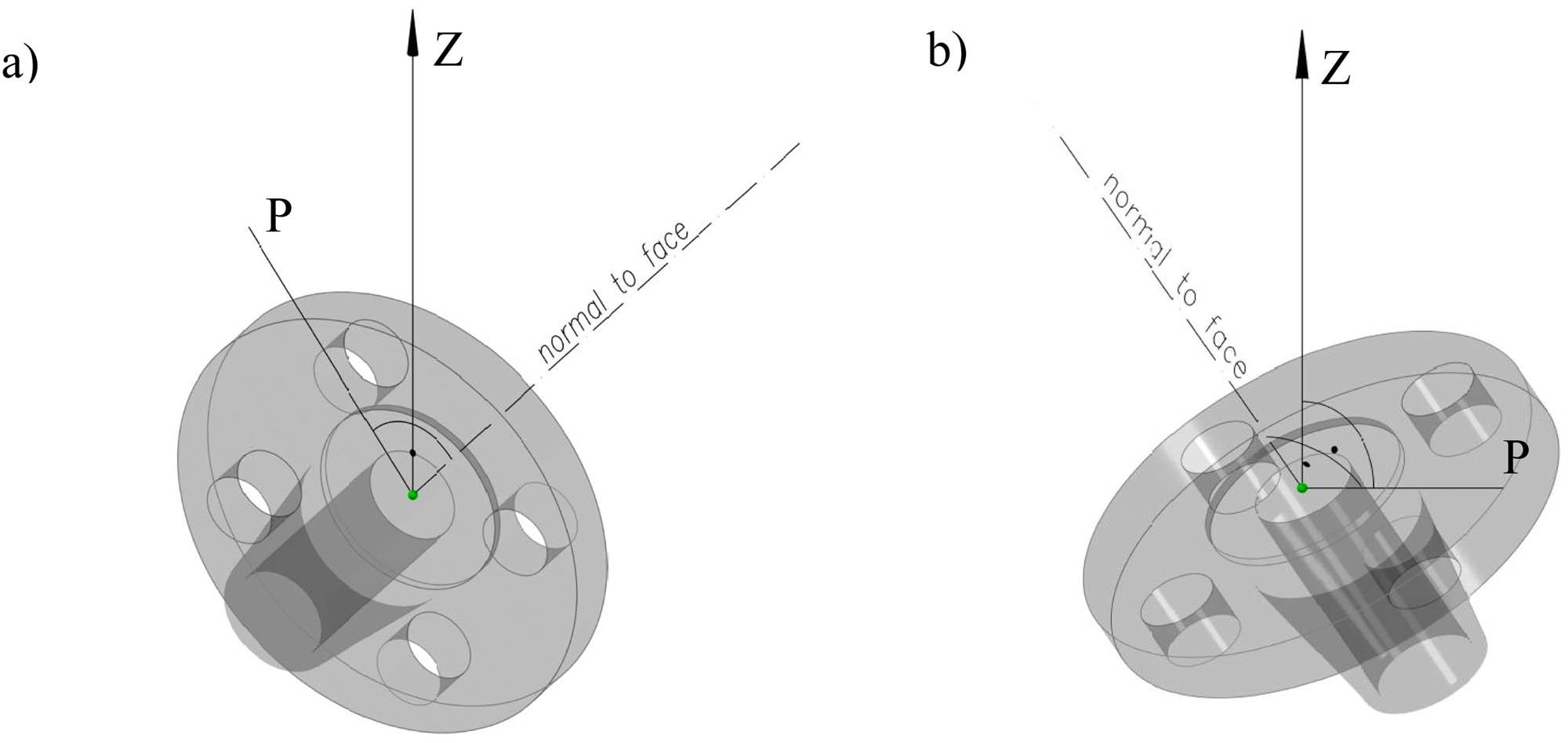
Two ways of P line definition: a) as the line of intersection of the vertical plane containing the TP and normal to face; b) as the line of intersection of the horizontal plane containing the TP.

The straight line M can also be defined in two ways. For flanges referred to in the project documentation as “one-bolt square” this is the same as the straight line B₁ connecting the flange TP with the center of the hole near the line P (Figure 5b). For flanges referred to as “two-bolt square” it is a bisector of an angle between lines B₁ and B₂, where the lines B₁ and B₂ pass through the TP and the bolt hole centers (Figure 5a).

Figure 5

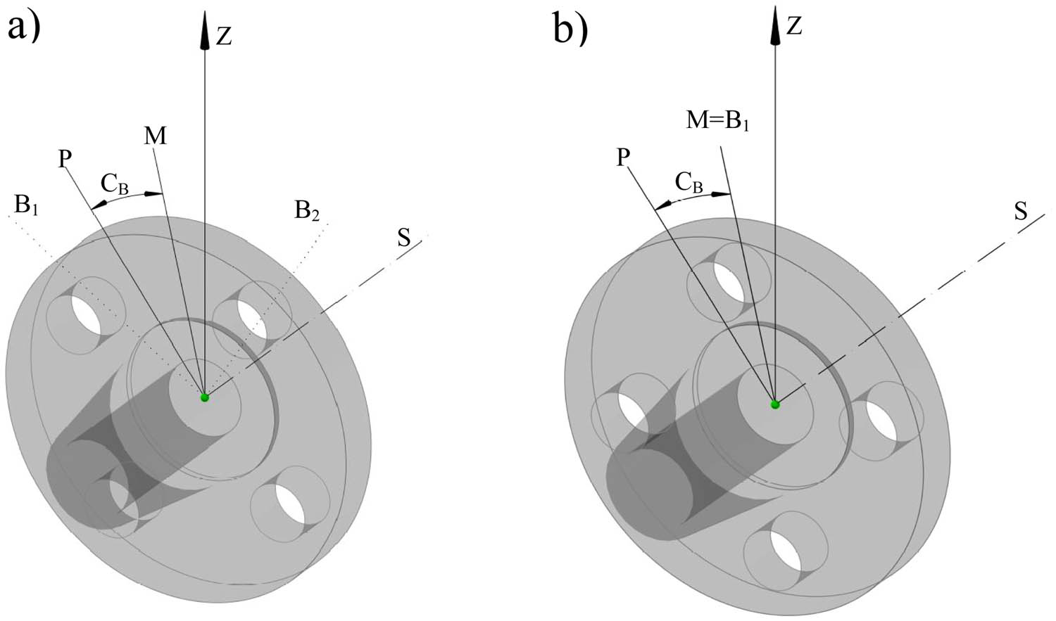
Two ways of M line definition: (a) two-bolt square flange; (b) one-bolt square flange.

5 Flange description for isometric transformation

The concept of isometric transformation assumes that both input data and result data are sets of points with XYZ coordinates; therefore, before using the transformational procedures it is necessary to change the description of the flange and to define it using a set of coordinates. It is vital to select points that should be located so as to clearly define the position, direction and rotation of the flange. The correction values of individual coordinates describing the flange, used in the objective function, should be proportional to the corrections of other points defining the spool.

Too large or too small correction values of the points describing the flange could give an effect similar to increasing or decreasing the LSM weight of the flange in the transformation process of the whole spool.

When describing the measured flange, the design values of the flange parameters defined in the previous chapter and deflections from these values are often given. Although basically all (except the coordinates of the TP) the parameters are angular values, the deflections are determined in millimeters as the displacement on the edge of the flange. Such a method of providing deflections facilitates their interpretation by workers who build prefabricates in a factory. In order to maintain proper proportions between corrections received during the transformation process, the points describing the flange should be chosen in such a manner that the size of corrections correspond to the linear values of deflections on the edge of the flange. Thus, points describing the flange are as follows (Figure 6):

1. Defining the position of the flange – TP.

2. Determining the direction of the flange’s face – point D located at the end of the normal vector of the face attached at the TP with a length equal to the flange radius. The components of the normal vector can be calculated from the horizontal and vertical bearing parameters as:

   (8)N=ABC=sin(BHz)cos(BV)cos(BHz)cos(BV)sin(BV).

   The coordinates of point D = [X_D, Y_D, Z_D]^T are calculated based on the coordinates of the point TP = [X_TP, Y_TP, Z_TP]^T:

   (9)D=TP+N⋅r

   where r denotes the radius of the flange’s face.

3. Flange’s rotation – point B located at the intersection of the edge of the face and the line joining the TP and the center of the bolt hole. Only one such point would be sufficient to determine the rotation; however, due to the problems with the identification of corresponding holes, described later in this article, it is necessary to determine the coordinates of points for all holes.

Figure 6

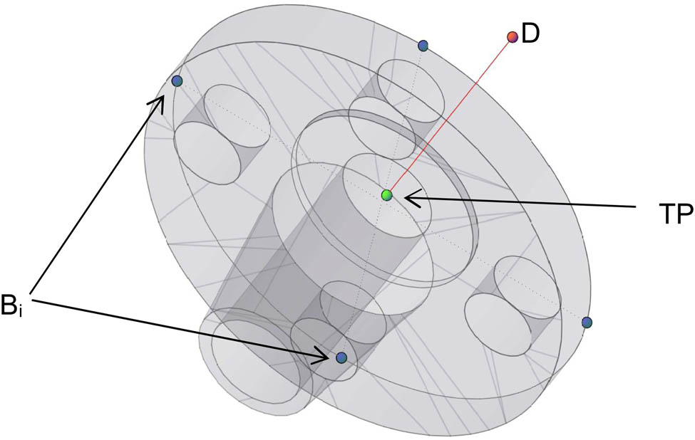
Points describing the flange for transformation needs.

The determination of the coordinates of the point starts from the calculation of the vector P connecting the TP and the edge of the flange (Figure 4). Assuming that the P is defined as the line of intersection of the horizontal plane containing the TP with the flange’s face (Figure 4b), then it is calculated as the cross product of the vertical unit vector and the normal vector:

Then vector P is scaled, so that it has a length equal to flange’s face radius r:

In the next step, the coordinates of the points B_i = [X_B, Y_B, Z_B]^T for n successive bolt holes are calculated as:

where:

i – bolt hole index,

β_n – the angle between the adjacent holes which is calculated as 360°/n (n is the number of bolt holes),

β_s – the angle between the vector P_r and the line connecting the TP and the center of the hole closest to P_r. Depending on the type of flange, it is: 0 for “one-bolt square flange” or β_n/2 for “two-bolt square flange.”

F(V₁, V₂, β) – a function whose task is to rotate vector V₁ around vector V₂ by an angle β. In practice, it can be implemented in various ways. An example of the implementation of such a function can be found in ref. [18]

6 Comparison of spools

In the proposed comparison method, we use two sets of coordinates of points defining the entire set as the input data: design ones and those in a system related to the place of measurement. Both sets contain mainly points describing the intersections of the axes of straight pipes (elbows), points describing the flanges and possibly other points relevant to the shape of the spool. These sets are treated as control points and, based on them, isometric transformation together with robust estimation are conducted (compare the formulas (6)). Thanks to the robust estimation, the largest deflections are expected at outliers’ points, while deflections should be small on elements matching each other. This meets the assumptions made at the beginning of the article.

Correct preparation of input data requires pairing the control points from both sets. If the whole process is to be carried out automatically, this can be done, e.g., by keeping an identical naming system of control points in the project and in the data from the measurement. However, there is a problem with the correct identification of corresponding bolt holes. The individual holes are not distinguished in any “physical” way. Therefore, it is difficult to develop a naming system that would allow for unambiguous matching of corresponding holes as early as at the stage of measuring the flange which is built.

The solution is to perform an isometric transformation twice. For the first time, the points defining the position of the bolt holes (12) are excluded from the set of control points. The coordinates of these points are only transformed to the output coordinate system based on the transformation parameters determined on the basis of the remaining points. Then the holes lying closest to each other (after transformation) are “paired” and considered corresponding to each other. In the next step, one pair of points defining one hole is added to the original (before transformation) sets of control points and the final transformation is performed along with the robust estimate. The remaining points determining the location of the holes are rejected because basically each of them carries similar information about the flange’s rotation; therefore, using more than one is not justified.

The last step is to compare the values of coordinates and angles describing the flanges and the whole set after transformation (in the output system). For this purpose, it is necessary to recalculate the angular parameters of the flange based on the coordinates describing it. Horizontal bearing B_Hz can be calculated as:

where α = arccos(A/r); A = X_D − X_TP; B = Y_D − Y_TP.

Vertical bearing is, respectively:

where C = Z_D − Z_TP.

Flange’s rotation C_B can be calculated as the spatial angle between the P vector and the vector between the TP and the B point that lies closest to the P vector.

7 Discussion

The proposed method allows to accelerate and improve the comparison of two steel pipe spools by eliminating the time-consuming and experience-dependent iterative process of moving, rotating and matching characteristic points. Thanks to the use of robust estimation, and it is possible to match spools, so that there are relatively few discrepancies (which, however, can reach significant values). This allows to minimize the number of corrections necessary to apply during the production of pipe spools and thus facilitates the entire construction process.

However, some doubts can be raised. The most important is the inability to unequivocally and quantitatively estimate the quality of the comparison method for spools. There is no single, clearly defined parameter that would make possible to unambiguously state that one method is better than the other. It is not root mean square error (RMSE) based on the deviations between matched models because the goal is not the best fit of both models but to find the minimum amount of corrections. Furthermore, the result of the comparison made by the manual method depends to a large extent on the experience of the survey engineer. Thus, it cannot be unequivocally stated that method described in this article gives numerically better results than the manual method.

A similar problem applies to every application of methods based on robust estimation. On the other hand, practical experience with such methods is definitely positive. They usually speed up the search for mistakes in observational data. In the case of a comparison of spools, fragments of structures that do not fit the project are treated similar to outliers’ observations. Thus, it should be expected that the use of the automatic comparison method will not only significantly reduce the time but also make it easier to find outliers.

Other problems related to the use of this type of method are primarily associated with the possible unstable solution of the system of equations. The simplest spool is a pipe at the ends of which two flanges are placed. A small number of points describing such an element and unfavorable geometry (the points are stretched along one straight line) may cause some numerical problems with correct solution of normal equations.

Despite the doubts expressed above regarding the subjectivity of quality assessment of various spool fitting methods, the proposed method has been implemented in commercial software GEONET Dimensional Control and is currently in the phase of practical tests on real objects.

It seems that in future, it would be useful to extend the method described above with the possibility of weighing selected points or elements of the flange (e.g., all points describing a given flange). Often, spools are built in stages. After the final welding of some part of the spool, further elements are added. During further work, it is assumed that it is not possible to move previously welded fragments; therefore, all corrections suggested by the survey engineer should apply only to the parts not yet welded. In such a situation, a significant increase in the weight of some of the points would result in the fixing of the already existing elements and possible deflections would be shown mainly on newly added fragments.

8 Conclusions

The publication proposes a comparison method of spools, which allows for the automation of a time-consuming part of the production process which is the comparison of the spool to be constructed with the design. The method aims to find non-matching elements and requires description of both spools using a set of coordinates of points. In particular, this applies to flanges, the direction and rotation of which are normally described by means of angular values. The method assumes that non-matching elements can be treated similarly to outliers observed in classical surveying tasks. Thus, the isometric transformation together with the robust estimation facilitate such a comparison. A set of points measured on the spool being built and a set of points describing the designed spool are assumed as control points. The final comparison of the spools requires recalculation of the flanges to angular values.

The proposed method, despite some doubts concerning, first of all, the possible unfavorable distribution of control points and the lack of a clear parameter allowing the assessment of the comparison quality, seems to be a solution that will significantly assist and accelerate the work of a survey engineer during the construction of a pipe spool.

References

[1] Awange JL, Aduol FWO. An evaluation of some robust estimation techniques in the estimation of geodetic parameters. Surv Rev. 1999;35(273):146–62.10.1179/sre.1999.35.273.146Suche in Google Scholar
[2] Banaś M. A review of robust estimation methods applied in surveying. Geomat Environ Eng. 2012;6(4):13–22.10.7494/geom.2012.6.4.13Suche in Google Scholar
[3] Ghilani CD. Adjustment computations: spatial data analysis, 5th ed. Wiley; 2011.Suche in Google Scholar
[4] Huber P. Robust estimation of a location parameter. Ann Math Stat. 1964;35:73–101.10.1007/978-1-4612-4380-9_35Suche in Google Scholar
[5] Janicka J, Rapinski J. Msplit transformation of coordinates. Surv Rev. 2013;45(331):269–74.10.1179/003962613X13726661625708Suche in Google Scholar
[6] Kadaj R. Eine verrallgemeinerte Klasse von Schatzverfahren mit praktuschen Anwendungen. ZfV4; 1988.Suche in Google Scholar
[7] Kadaj R. Rozwinięcie koncepcji niestandardowej metody estymacji. Geodezja i Kartogr. 1980;XXIX(3–4):185–96.Suche in Google Scholar
[8] Kamiński W, Wiśniewski Z. Analiza wybranych, odpornych na błędy grube, metod wyrównania obserwacji geodezyjnych. Geodezja i Kartogr. 1992;XLI(3–4):173–81, and 183–95.Suche in Google Scholar
[9] Karsznia K. Geodezyjny monitoring obiektów mostowych. Mosty. 2011;6:36–42.Suche in Google Scholar
[10] Krarup T. The danish method, experience and philosophy. DGK Heft; 1983. p. 98.Suche in Google Scholar
[11] Kwaśniak M. Effectiveness of chosen robust estimation methods compared to the level of network reliability. Geodesy Cartography. 2011;60:3–19.10.2478/v10277-012-0014-9Suche in Google Scholar
[12] Mrówczyńska M. Identyfikacja układu odniesienia sieci niwelacyjnej obszaru legnicko-głogowskiego okręgu miedziowego. Acta Sci Pol Geodesia et Descriptio Terrarum. 2010;9(4):27–36.Suche in Google Scholar
[13] Muszyński Z, Mąkolski K, Osada W. Zastosowanie metod estymacji odpornej w geodezyjnych pomiarach pionowych przemieszczeń obiektów budowlanych. Acta Sci Pol,Geodesia et Descriptio Terrarum. 2005;4(1):85–97.Suche in Google Scholar
[14] Nahangi M, Haas CT. Automated 3D compliance checking in pipe spool fabrication. Adv Eng Inform. 2014;28:360–9.10.1016/j.aei.2014.04.001Suche in Google Scholar
[15] Safa M, Shahi A, Nahangi M, Haas CT, Noori H. Automating measurement process to improve quality management for piping fabrication. Structures. 2015;3:71–80.10.1016/j.istruc.2015.03.003Suche in Google Scholar
[16] Sato M, Kojima H. Using laser radar to improve production in pipe spool fabrication. Quality Digest. 2012. Retrieved from https://www.qualitydigest.com/inside/cmsc-article/using-laser-radar-improve-production-pipe-spool-fabrication-081512.html (access: 2019.08.10).Suche in Google Scholar
[17] Shiliang Z, Jin Y. Measurement and quick replacement of pipeline segments in an offshore platform. In: Advanced Materials Research. Vol. 261–263, Trans Tech Publications; 2011. p. 1406–9.10.4028/www.scientific.net/AMR.261-263.1406Suche in Google Scholar
[18] Steven JL. Linear algebra with applications, 9th ed. Pearson Education Limited; 2015.Suche in Google Scholar
[19] Świętoń T, Oleniacz G. Accuracy of steel flanges measurement in renovation and construction work for offshore industry. J Surveying Eng. 2020;146(2):04020006-1–04020006-11.10.1061/(ASCE)SU.1943-5428.0000310Suche in Google Scholar
© 2020 Świętoń Tomasz et al., published by De Gruyter
This work is licensed under the Creative Commons Attribution 4.0 International License.
Artikel in diesem Heft
- Regular Articles
- The simulation approach to the interpretation of archival aerial photographs
- The application of137Cs and210Pbexmethods in soil erosion research of Titel loess plateau, Vojvodina, Northern Serbia
- Provenance and tectonic significance of the Zhongwunongshan Group from the Zhongwunongshan Structural Belt in China: insights from zircon geochronology
- Analysis, Assessment and Early Warning of Mudflow Disasters along the Shigatse Section of the China–Nepal Highway
- Sedimentary succession and recognition marks of lacustrine gravel beach-bars, a case study from the Qinghai Lake, China
- Predicting small water courses’ physico-chemical status from watershed characteristics with two multivariate statistical methods
- An Overview of the Carbonatites from the Indian Subcontinent
- A new statistical approach to the geochemical systematics of Italian alkaline igneous rocks
- The significance of karst areas in European national parks and geoparks
- Geochronology, trace elements and Hf isotopic geochemistry of zircons from Swat orthogneisses, Northern Pakistan
- Regional-scale drought monitor using synthesized index based on remote sensing in northeast China
- Application of combined electrical resistivity tomography and seismic reflection method to explore hidden active faults in Pingwu, Sichuan, China
- Impact of interpolation techniques on the accuracy of large-scale digital elevation model
- Natural and human-induced factors controlling the phreatic groundwater geochemistry of the Longgang River basin, South China
- Land use/land cover assessment as related to soil and irrigation water salinity over an oasis in arid environment
- Effect of tillage, slope, and rainfall on soil surface microtopography quantified by geostatistical and fractal indices during sheet erosion
- Validation of the number of tie vectors in post-processing using the method of frequency in a centric cube
- An integrated petrophysical-based wedge modeling and thin bed AVO analysis for improved reservoir characterization of Zhujiang Formation, Huizhou sub-basin, China: A case study
- A grain size auto-classification of Baikouquan Formation, Mahu Depression, Junggar Basin, China
- Dynamics of mid-channel bars in the Middle Vistula River in response to ferry crossing abutment construction
- Estimation of permeability and saturation based on imaginary component of complex resistivity spectra: A laboratory study
- Distribution characteristics of typical geological relics in the Western Sichuan Plateau
- Inconsistency distribution patterns of different remote sensing land-cover data from the perspective of ecological zoning
- A new methodological approach (QEMSCAN®) in the mineralogical study of Polish loess: Guidelines for further research
- Displacement and deformation study of engineering structures with the use of modern laser technologies
- Virtual resolution enhancement: A new enhancement tool for seismic data
- Aeromagnetic mapping of fault architecture along Lagos–Ore axis, southwestern Nigeria
- Deformation and failure mechanism of full seam chamber with extra-large section and its control technology
- Plastic failure zone characteristics and stability control technology of roadway in the fault area under non-uniformly high geostress: A case study from Yuandian Coal Mine in Northern Anhui Province, China
- Comparison of swarm intelligence algorithms for optimized band selection of hyperspectral remote sensing image
- Soil carbon stock and nutrient characteristics of Senna siamea grove in the semi-deciduous forest zone of Ghana
- Carbonatites from the Southern Brazilian platform: I
- Seismicity, focal mechanism, and stress tensor analysis of the Simav region, western Turkey
- Application of simulated annealing algorithm for 3D coordinate transformation problem solution
- Application of the terrestrial laser scanner in the monitoring of earth structures
- The Cretaceous igneous rocks in southeastern Guangxi and their implication for tectonic environment in southwestern South China Block
- Pore-scale gas–water flow in rock: Visualization experiment and simulation
- Assessment of surface parameters of VDW foundation piles using geodetic measurement techniques
- Spatial distribution and risk assessment of toxic metals in agricultural soils from endemic nasopharyngeal carcinoma region in South China
- An ABC-optimized fuzzy ELECTRE approach for assessing petroleum potential at the petroleum system level
- Microscopic mechanism of sandstone hydration in Yungang Grottoes, China
- Importance of traditional landscapes in Slovenia for conservation of endangered butterfly
- Landscape pattern and economic factors’ effect on prediction accuracy of cellular automata-Markov chain model on county scale
- The influence of river training on the location of erosion and accumulation zones (Kłodzko County, South West Poland)
- Multi-temporal survey of diaphragm wall with terrestrial laser scanning method
- Functionality and reliability of horizontal control net (Poland)
- Strata behavior and control strategy of backfilling collaborate with caving fully-mechanized mining
- The use of classical methods and neural networks in deformation studies of hydrotechnical objects
- Ice-crevasse sedimentation in the eastern part of the Głubczyce Plateau (S Poland) during the final stage of the Drenthian Glaciation
- Structure of end moraines and dynamics of the recession phase of the Warta Stadial ice sheet, Kłodawa Upland, Central Poland
- Mineralogy, mineral chemistry and thermobarometry of post-mineralization dykes of the Sungun Cu–Mo porphyry deposit (Northwest Iran)
- Main problems of the research on the Palaeolithic of Halych-Dnister region (Ukraine)