Inverse-designed gyrotropic scatterers for non-reciprocal analog computing
-
Nikolas Hadjiantoni
 ,
Heedong Goh
,
Stephen M. Hanham
,
Heedong Goh
,
Stephen M. Hanham
 and
Andrea Alù
and
Andrea Alù

Abstract
While conventional von Neumann based machines are increasingly challenged by modern day requirements, electromagnetic analog computing devices promise to provide a platform that is highly parallel, efficient and fast. Along this paradigm, it has been shown that arrays of subwavelength electromagnetic scatterers can be used as solvers of partial differential equations. Inverse design offers a powerful tool to synthesize such analog computing machines, utilizing engineered non-local responses to produce the solution of a desired mathematical operation encoded in the scattered fields. So far, this approach has been largely restricted to linear, reciprocal scatterers, limiting its generality and applicability. Here we demonstrate how arrays of gyrotropic scatterers can be used to solve a more general class of differential equations. Through inverse design, with a combination of evolutionary and gradient based algorithms, the position of the scatterers is optimized to achieve the desired kernel response. Introducing gyrotropic media, we also demonstrate improved accuracy by >2 orders of magnitude compared to similarly sized reciprocal systems designed with the same method.
1 Introduction
While the demand to process data is increasing at an unprecedented rate, von Neumann based computers are proving to be simultaneously energy inefficient and overly time consuming [1], [2]. Between 2011 and 2022, the average computation required by machine learning systems has increased from 1016 floating point operations per second (FLOPS) to 1024 FLOPS, [3]. This indicates a significant need to increase the energy efficiency and time cost of mathematical operations.
In an attempt to remove such a bottleneck from the development of computational models, recent works have explored the use of photonic scatterers, metamaterials and metasurfaces to take advantage of their fast and highly efficient response to model integro-differential problems, recurrent neural networks (RNNs) and extreme learning machines [2], [4], [5], [6], [7], [8], [9], [10], [11], [12], [13], [14]. Since such optical systems yield massively parallel, high-speed and energy efficient operations, these photonic devices have proven to be a promising surrogate for their von Neumann based counterparts [1].

Non-reciprocal scatterer composed of two types of cylinders, gyrotropic and dielectric cylinders, returning a solution u = A −1 f encoded within a scattered wave.
By embedding the underlying mathematical problem in the properties of the incoming field, analog computing devices can shape the field distribution by fine-tuning their spatial and temporal parameters to achieve a desired response [12]. The response can be thought of as a kernel acting on the input distribution that approximates a linear mathematical operator or its inverse. In this context, inverse design has been drawing significant interest in the quest of developing analog computing optical machines, due to its ability to find non-trivial solutions for such scatterers [5], [15], [16], [17]. As shown in previous work [8], odd-symmetric mathematical operators require breaking both transverse and longitudinal symmetries. For this reason, inverse-designed structures with broken symmetries offer an ideal design playground for these devices [18]. So far, however, they have been limited to the solution of linear integro-differential equations [19].
As another limitation, the meta-structures considered so far have relied on reciprocal media, where reciprocity indicates the inherent symmetry in optical response as source and observation points are exchanged. While a good number of relevant mathematical problems obey sufficient symmetries to be synthesized using reciprocal optical responses, breaking reciprocity can enable a wider range of operations, relevant for instance in the context of machine learning, thermodynamics and cosmology [20], [21], [22]. In this manuscript, we introduce an analog computing framework that harnesses nonreciprocal scattering induced by a static magnetic bias on an array of scatterers (Figure 1), with the goal of expanding the rational synthesis of analog optical computers based on engineered nonlocalities.
2 Methods
Here, we describe the analytical procedures for formulating the wave–scatterer interaction into a scattering-matrix representation and for discretizing the target mathematical problem into a matrix form. Subsequently, we establish the relationship between the two system matrices, which guides the design process of the scatterer.
2.1 Ensemble of gyrotropic particles
The geometry for the proposed analog computing framework is described by a two-dimensional problem in which we assume that the fields are transverse electric (TE), which can be reduced to a scalar Helmholtz equation in terms of the magnetic field component H z . We compose the scatterer by a system of small particles, where each particle is approximated by a dipole moment.
The polarizability of each particle is derived from the dominant scattering coefficients. We consider a single circular scatterer in a vacuum with radius a. The solution to an incident plane wave with e iωt dependency reads
where J
n
and
where
Scattering coefficients for both gyrotropic and dielectric media can be described by the same expression [23]
In the above, ɛ
0 and
The scattering coefficients S
n
of order −1, 0, and 1 dominate the responses when the radius is much smaller than the background wavelength, i.e., a ≪ λ
0. Then, we can approximate the scatterer by dipole moments, where the relation between their amplitude d = [m, p]
T
and the incident field
Here, m and p are magnetic and electric dipoles, respectively, and α is the polarizability tensor. Without loss of generality, due to the small size of the scatterers, no coupling between H and E is assumed, i.e., α 01 = α 10 = 0. Then, as shown in Appendix A.2, we have
In the above, we have S −1 = −S 1 for a dielectric case, which implies reciprocity.
According to [25], the magnetic and electric field induced by a dipole can be expressed by F scat = Γd or
where Γ is the dipole-dipole interaction matrix that maps a dipole to a scattered field (Appendix A.3).
The multi-scatterer generalization of eq. (5) for ith particle can be written as
Here, the effective incident wave for the ith particle
Here, each element of D is the dipole moment d = [m p] T induced by each particle. Each component of the vector P corresponds to the incident field F inc sampled at the position of each particle:
where Ω is the domain that contains all particles and δ(x − x i ) is a Dirac delta.
Similarly, the generalization of (7) for an arbitrary position x with an N-particle system is
where each interaction matrix
The incident field can be expanded in a functional basis of our choice [5], [12], [25], that is, expressed as a summation of basis functions with distinct coefficients. These coefficients serve as control variables encoding the input signal [5]. Then, the complexity of the problem is governed by the number of input and output ports. Let B n (x) = J n (k 0 r)e in(ϕ−θ) represents the basis for the incident magnetic field H inc, or the input ports. Then, the expansion reads
where
Likewise, the choice of output ports is motivated by the general solution of the scattered field in an exterior problem, i.e.,
where
It is noted that the choice of basis functions is, in general, arbitrary; the above selection ensures completeness for the two-dimensional problem [27].
Let
or in tensor form,
The scattering matrix S mn is a linear operator mapping the input vector c in to the output vector c out .
2.2 Mathematical problem
The target linear mathematical problem for any ODE can be stated as
where A is the operator acting on an unknown function u and f is a given function. The operator A is not necessarily self-adjoint, which may describe a nonreciprocal physical problem. For example, we consider the following operator, which represents a typical form of a second-order boundary value problem:
with two complex-valued parameters α and β and the periodic boundary condition over 2π. In the weak form, the above strong form can be expressed as
In the above, v denotes a test function, and V is a set of admissible functions.
Among many choices of finite-dimensional approximations, we take Rayleigh-Ritz type discretization, which reads
The expansion is evaluated at the interface with a radius of choice r = a. The above basis choice implies that we use sinusoidal basis for both input and output ports in (13) and (15). Thus, f is now expressed with a finite series of sinusoidal functions representing the input.
Using this result, eq. (18) can be approximated to a matrix equation
where u and f are the vectors of the coefficients u
n
, f
n
defined in eq. (21), respectively. The operator
A
is the finite approximation of the operator
The aim is to design a scatterer such that its geometry maps the response of eq. (22) to its scattering matrix in a way that the solution is imprinted on the scattering fields when illuminated by incident fields f. Therefore, the scattering matrix S should satisfy
where I is the identity matrix and γ is a scaling factor [5].
2.3 Scatterer design
The position of the particles can be formed as an inverse design problem. From eq. (24), it follows that the cost function for this inverse design problem can be formulated as
where
where
A two-step optimization process is used as shown in Figure 2 and the code can be found in [28]. The framework was implemented using the open source library NLopt in Python [29]. First, an optimization is performed using the global evolutionary algorithm (ESCH) [30] followed by the gradient based method of moving asymptotes (MMA) [31]. As a global optimizer is better suited to exploring a larger part of the parameter space, introducing it at the beginning allows for better exploration of a wider region of possible solutions. However, as global optimizers often suffer from slow convergence, the gradient based optimizer allows for faster convergence to the local minima of the region that the ESCH algorithm identified. The hybrid method explores the solution space more efficiently and accurately than deploying either of the algorithms on an individual basis [32].
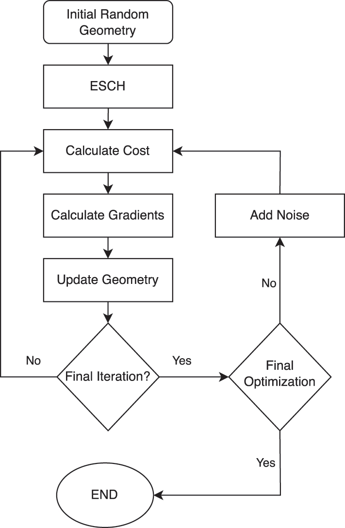
Optimization algorithm for the positions of the cylinders.
The calculation of gradients δq, required by MMA, was performed using finite differences. Given the small number of elements in vector q, the problem did not necessitate the use of the adjoint variable method. To reduce the computational time required, the process was parallelized using mpi4py [33] to calculate each element of δq on a different simultaneous process.
Random noise was integrated in the optimization process to encourage tolerance in the solution, yielding more robust devices. The gradient based optimizer was employed 10 times with a maximum number of iterations at 1,000 per optimization session. Each time the position vector with the lowest cost function was used with added noise i.e.
where q best is the best performing geometry from the previous iterations and Y is a random variable vector and Y k is the kth element of Y. This can also be considered a fabrication robustness measure, with geometries who are less susceptible to this perturbation being favored as the starting point for the next optimization.
3 Results
Using the quasi-static dipolar resonant condition from [23], the design frequency of ω = 1 × 10¹² rad s−1 was chosen with ω p = 2.1 × 10¹² rad s−1 and ω c = 0.57ω p for gyrotropic cylinders, and loss-less silicon as the dielectric material with ɛ = 12ɛ 0, ω c = 0 for a 7 harmonics system. The optimization region is a 20λ 0 × 20λ 0 square as shown in Figure 3. The figure also shows how the scatterer interacts with the 7 incoming spherical harmonics to map the solution to the scattered fields.
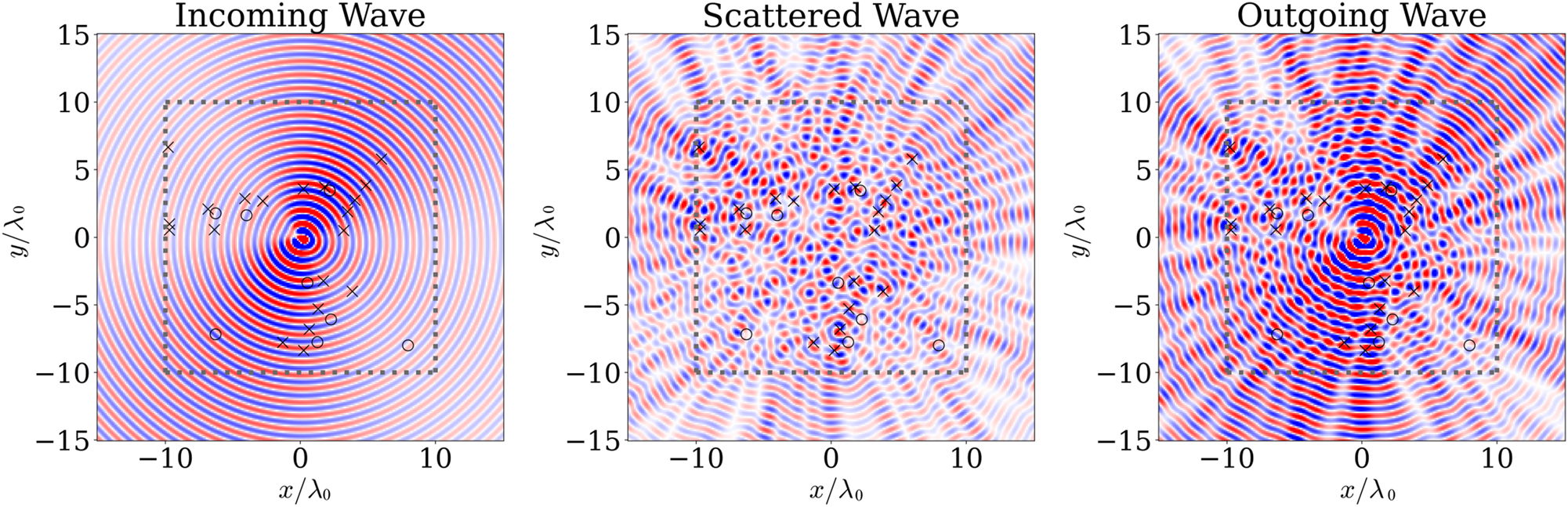
Plot showing the incoming, scattered and outgoing H z from an analog computing scatterer. The dashed line shows the optimization region, ‘x’ represents gyrotropic scatterers, while ‘o’ represents dielectric scatterers.
The scatterer in Figure 3 shows the incident and scattered fields to a scatterer constructed with a
The performance of the scatterer was tested using two input functions f a,b .
where each element represents the value at
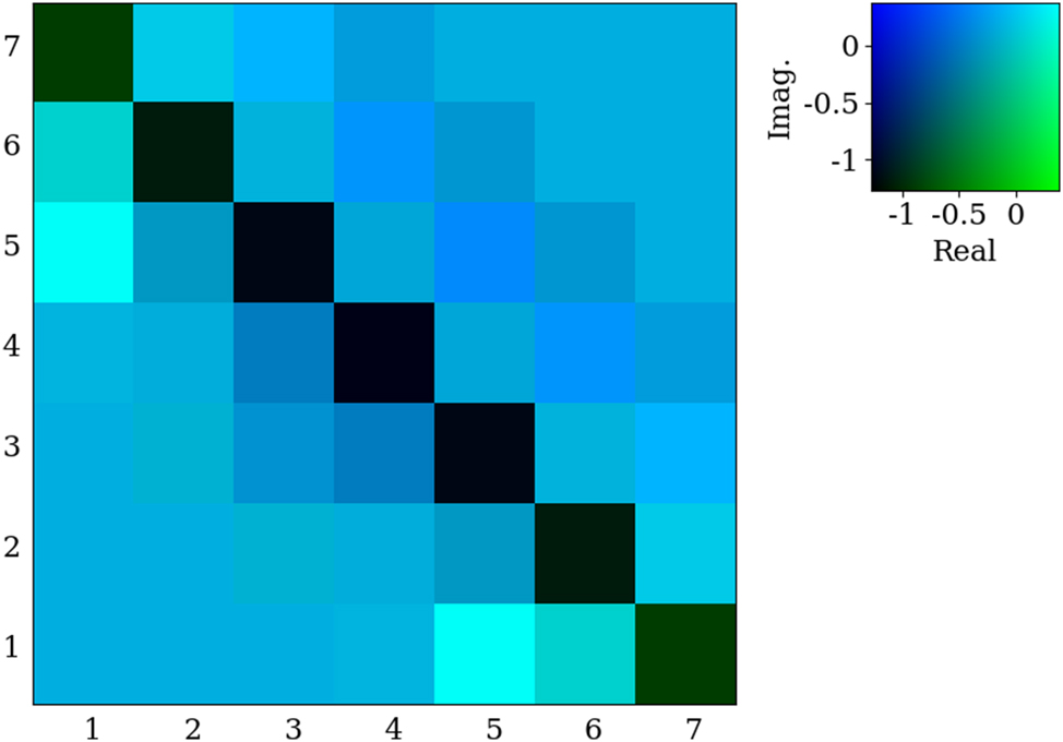
Example inverse non-Hermitian kernel used in the cost function to map the scattering matrix on the scatterer’s geometry using eq. (25).
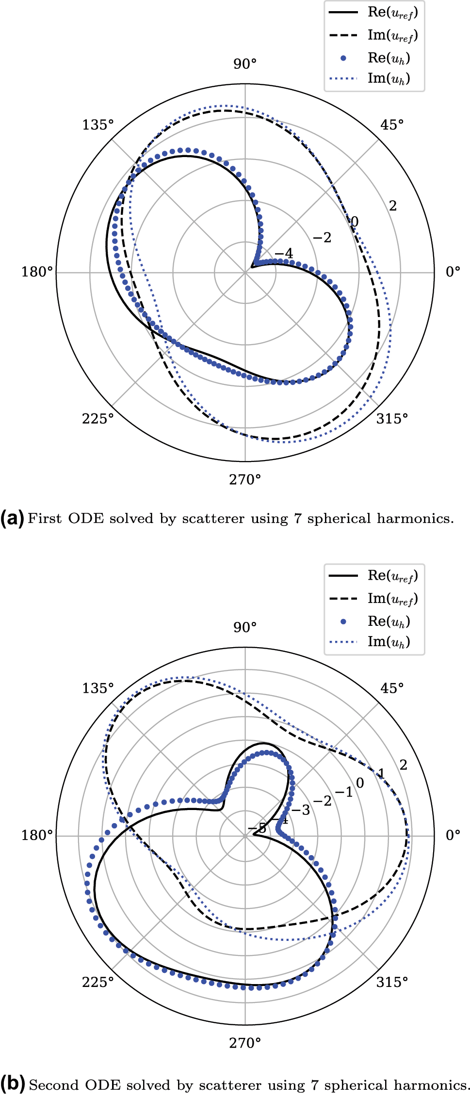
Solution to two different ODEs by the same scatterer shown in Figure 3. (a) First ODE solved by scatterer using 7 spherical harmonics. (b) Second ODE solved by scatterer using 7 spherical harmonics.
Figure 5 shows two solutions of ODEs from the same scatterer, the design of the scatterer is shown in Figure 3. In both cases the solution of the analog solver closely matches the numerical solution. Both problems have increased complexity compared to previously demonstrated analog computing scatterers [5]. Compared to numerical solutions, a 5 by 5 scatterer achieved a maximum error of ∼1 %, while for the 7 by 7 scatterer presented here, the maximum error was ∼3 %. While the accuracy of numerical solutions, such as u ref, depends on a range of factors, it is generally accepted that they can achieve accuracies ≪1 % [34]. The authors believe, however, that the permitted trade-off between accuracy and efficiency, as well as their compactness make this approach attractive for implementing future analog computing devices.
To understand whether gyrotropic media are essential for the solution of generally asymmetric ODEs, their performance was compared to scatterer geometries with an ensemble of perfect electric conductor (PEC) and dielectric cylinders. Since gyrotropic media are PEC with an external magnetic bias, the initial conditions of the previous experiment are repeated, without the external magnetic bias. Figure 6 shows the performance of the best design for each case for different numbers of scatterer particles. The use of non-reciprocal media clearly results in improved performance for the solution of non-reciprocal ODEs. Using gyrotropic cylinders consistently gives a lower cost function by more than an order of magnitude (or 95 % reduction). It is noted that in both cases there is slight fluctuation, believed to be due to: (a) random starting conditions, (b) increasing the number of optimization parameters, and (c) the ability of a larger number of particles to populate larger matrices. Using the literature value for the lossy permittivity of high resistivity silicon at ω = 1 THz, ɛ = 11.66 + 2.4i × 10−3 [35] results in a difference <1 % in the cost function for all numbers of particles, demonstrating the robustness of the solution.
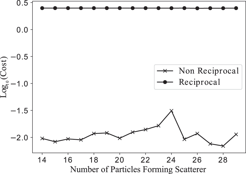
The logarithm of the smallest achieved cost function of eq. (25) when optimizing with gyrotropic media (non-reciprocal) or perfect electric conductors (reciprocal).
To test the robustness of the system, the optimal solution was perturbed using eq. (27) with Y again generated using a uniform random distribution with boundaries
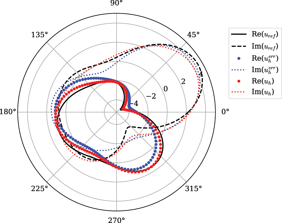
Comparison of the performance of the scatterer with the ideal solution (black), unperturbed scatterer (red) and uniformly perturbed scatterer (blue).
The third example highlights not only the small deviation between perturbed scatterers’s solution to the unperturbed but also to the analytical solution. This robustness to errors in position is an important step towards a practical implementation of the analog computing device. This can be attributed to embedding noise in the optimization problem, biasing the final result to geometries that have small variations in solution under such errors.
4 Conclusions
In this paper, an inverse-design technique was used to create a system of gyrotropic and dielectric scatterers whose electromagnetic scattering characteristics can be used to implement an analog computing device capable of solving ODEs. The input function for the scatterer is encoded in the spherical harmonics of an incident electromagnetic wave that is scattered from the system. The solution can then be read from the spherical harmonics of the scattered fields. The optimal geometries were found using a combination of global and local optimizers to determine the position of the gyrotropic and dielectric cylinder scatterers. As a proof of concept, scatterers using 7 spherical harmonics were designed and tested against two different ODEs, and a reasonable level of accuracy was demonstrated.
Similar analog computing scatterers using PEC-only scatterers were optimized using the same method in order to understand the necessity of gyrotropic media. The PEC-based scatterers achieved cost functions higher than the gyrotropic based solutions by an order of magnitude. While the gyrotropic based scatterers showed an improved performance as the number of optimized parameters was increased, the PEC-based scatterers maintained the same level of performance.
Expanding on the ideas introduced by previous scattering-based analog computing devices [5], we used inverse design to develop non-reciprocal scattering based analog computers. We believe that these ultra-fast and compact devices can be deployed for problem-specific non-reciprocal applications.
Funding source: H2020 Excellent Science
Award Identifier / Grant number: 777714
Funding source: National Research Foundation of Korea
Award Identifier / Grant number: 0583-20250056
Acknowledgements
The computations described in this work were performed using the University of Birmingham’s BlueBEAR HPC service, which provides a High Performance Computing service to the University’s research community. See http://www.birmingham.ac.uk/bear for more details.
-
Research funding: This work was funded by EU’s Horizon 2020 Research and Innovation Program (Grant No. 777714). HG is partially supported by National Research Foundation of Korea (NRF) grant (No. 0583-20250056). HG and AA were supported by the Department of Defense.
-
Author contributions: All authors have accepted responsibility for the entire content of this manuscript and consented to its submission to the journal, reviewed all the results and approved the final version of the manuscript. NH and HG contributed equally. NH designed the optimization algorithm and wrote the manuscript. HG designed the numerical solvers and edited the manuscript. SMH, MNC and AA supervised and edited the manuscript.
-
Conflict of interest: Authors state no conflict of interest.
-
Data availability: Data and code underlying the results presented in this paper are available in NH and HG’s repository https://doi.org/10.5281/zenodo.15107584.
A Appendix
A.1 Permittivity and permeability for a gyrotropic medium
The permittivity and the permeability for a (piecewise) homogeneous gyrotropic medium reads [23]
In the above,
We assume a transverse-electric incident plane wave with no external current density, i.e.,
Then, the Maxwell’s equations are reduced to a two-dimensional Helmholtz equation in the z component of the vector field H, i.e.,
where the effective permittivity reads
A.2 Derivation of α 00 and α 11
Electric and magnetic fields due to an electric dipole moment located at ρ′ = (r′, ϕ′) are [25]
In the above, we have
Let ρ′ = 0 and considering only the electric dipole contribution of the scattered field, i.e. n = −1, 1, the left-hand-side of the (37) becomes
Note that we have S −1 = −S 1 for reciprocal cases. The right-hand-side of (37) becomes
Then, we have
On the other hand, the polarizability is defined as
where
Combining (42), (43), and (44), we have a system of linear equations, i.e.,
or
The solution to the above system of equations is
Next, we derive α 00 such that
where [25]
We assume that S 0, S −1, and S 1 dominate the response in (39). The contributions of S −1 and S 1 have been addressed previously. Thus, considering only the remaining S 0 term, we obtain
A.3 Elements of Γ
Expansion of the elements in eq. (7)
References
[1] D. Zhang and Z. Tan, “A review of optical neural networks,” Appl. Sci., vol. 12, no. 11, p. 5338, 2022. https://doi.org/10.3390/app12115338.Search in Google Scholar
[2] Y. Zhou, H. Zheng, I. I. Kravchenko, and J. Valentine, “Flat optics for image differentiation,” Nat. Photonics, vol. 14, no. 5, pp. 316–323, 2020. https://doi.org/10.1038/s41566-020-0591-3.Search in Google Scholar
[3] J. Sevilla, L. Heim, A. Ho, T. Besiroglu, M. Hobbhahn, and P. Villalobos, “Compute trends across three eras of machine learning,” in 2022 International Joint Conference on Neural Networks (IJCNN), IEEE, 2022.10.1109/IJCNN55064.2022.9891914Search in Google Scholar
[4] W. T. Chen, A. Y. Zhu, J. Sisler, Z. Bharwani, and F. Capasso, “A broadband achromatic polarization-insensitive metalens consisting of anisotropic nanostructures,” Nat. Commun., vol. 10, no. 1, p. 355, 2019. https://doi.org/10.1038/s41467-019-08305-y.Search in Google Scholar PubMed PubMed Central
[5] H. Goh and A. Alù, “Nonlocal scatterer for compact wave-based analog computing,” Phys. Rev. Lett., vol. 128, no. 7, p. 073201, 2022, https://doi.org/10.1103/physrevlett.128.073201.Search in Google Scholar
[6] T. W. Hughes, M. Minkov, V. Liu, Z. Yu, and S. Fan, “Full wave simulation and optimization of large area metalens,” in OSA Optical Design and Fabrication 2021 (Flat Optics, Freeform, IODC, OFT), https://doi.org/10.1364/flatoptics.2021.fth3c.5.Search in Google Scholar
[7] E. Khoram et al.., “Nanophotonic media for artificial neural inference,” Photonics Res., vol. 7, no. 8, pp. 823–827, 2019. https://doi.org/10.1364/prj.7.000823.Search in Google Scholar
[8] H. Kwon, D. Sounas, A. Cordaro, A. Polman, and A. Alù, “Nonlocal metasurfaces for optical signal processing,” Phys. Rev. Lett., vol. 121, no. 17, p. 173004, 2018. https://doi.org/10.1103/physrevlett.121.173004.Search in Google Scholar
[9] R. G. MacDonald, A. Yakovlev, and V. Pacheco-Peña, “Solving partial differential equations with waveguide-based metatronic networks,” Adv. Photonics Nexus, vol. 3, no. 5, p. 056007, 2024. https://doi.org/10.1117/1.apn.3.5.056007.Search in Google Scholar
[10] A. Momeni and R. Fleury, “Electromagnetic wave-based extreme deep learning with nonlinear time-floquet entanglement,” Nat. Commun., vol. 13, no. 1, p. 2651, 2022. https://doi.org/10.1038/s41467-022-30297-5.Search in Google Scholar PubMed PubMed Central
[11] Y. Shen et al.., “Deep learning with coherent nanophotonic circuits,” Nat. Photon., vol. 11, no. 7, pp. 441–446, 2016.10.1038/nphoton.2017.93Search in Google Scholar
[12] A. Silva, F. Monticone, G. Castaldi, V. Galdi, A. Alù, and N. Engheta, “Performing mathematical operations with metamaterials,” Science, vol. 343, no. 6167, pp. 160–163, 2014. https://doi.org/10.1126/science.1242818.Search in Google Scholar PubMed
[13] F. Zangeneh-Nejad, D. L. Sounas, A. Alù, and R. Fleury, “Analogue computing with metamaterials,” Nat. Rev. Mater., vol. 6, no. 3, pp. 207–225, 2021. https://doi.org/10.1038/s41578-020-00243-2.Search in Google Scholar
[14] P. Zhang, Y. Hu, Y. Jin, S. Deng, X. Wu, and J. Chen, “A Maxwell’s equations based deep learning method for time domain electromagnetic simulations,” IEEE J. Multiscale Multiphys. Comput. Tech., vol. 6, no. 1, pp. 35–40, 2021. https://doi.org/10.1109/jmmct.2021.3057793.Search in Google Scholar
[15] W. Gao et al.., “Topological photonic phase in chiral hyperbolic metamaterials,” Phys. Rev. Lett., vol. 114, no. 3, p. 037402, 2015, https://doi.org/10.1103/physrevlett.114.037402.Search in Google Scholar PubMed
[16] A. F. Oskooi, D. Roundy, M. Ibanescu, P. Bermel, J. D. Joannopoulos, and S. G. Johnson, “Meep: A flexible free-software package for electromagnetic simulations by the fdtd method,” Comput. Phys. Commun., vol. 181, no. 3, pp. 687–702, 2010. https://doi.org/10.1016/j.cpc.2009.11.008.Search in Google Scholar
[17] T. Zhu et al.., “Topological optical differentiator,” Nat. Commun., vol. 12, no. 1, p. 680, 2021. https://doi.org/10.1038/s41467-021-20972-4.Search in Google Scholar PubMed PubMed Central
[18] A. Cordaro, B. Edwards, V. Nikkhah, A. Alù, N. Engheta, and A. Polman, “Solving integral equations in free space with inverse-designed ultrathin optical metagratings,” Nat. Nanotechnol., vol. 18, no. 4, pp. 365–372, 2023, https://doi.org/10.1038/s41565-022-01297-9.Search in Google Scholar PubMed
[19] N. M. Estakhri and A. Alù, “Wave-front transformation with gradient metasurfaces,” Phys. Rev. X, vol. 6, no. 4, p. 041008, 2016. https://doi.org/10.1103/physrevx.6.041008.Search in Google Scholar
[20] N. Boullé, D. Halikias, S. E. Otto, and A. Townsend, “Operator learning without the adjoint,” J. Mach. Learn. Res., vol. 25, no. 364, pp. 1–54, 2024, http://jmlr.org/papers/v25/24-0162.html.Search in Google Scholar
[21] H. Alston, L. Cocconi, and T. Bertrand, “Irreversibility across a nonreciprocal p t -symmetry-breaking phase transition,” Phys. Rev. Lett., vol. 131, no. 25, p. 258301, 2023. https://doi.org/10.1103/physrevlett.131.258301.Search in Google Scholar
[22] F. Masghatian, M. Esfandiar, and M. Nouri-Zonoz, “Electrodynamics in curved spacetime: Gravitationally-induced constitutive equations and the spacetime index of refraction,” Class. Quantum Grav., vol. 42, no. 12, p. 125002, 2025, https://doi.org/10.1088/1361-6382/addcb1.Search in Google Scholar
[23] C. Valagiannopoulos, S. A. H. Gangaraj, and F. Monticone, “Zeeman gyrotropic scatterers: Resonance splitting, anomalous scattering, and embedded eigenstates,” Nanomater. Nanotechnol., vol. 8, no. 1, 2018, https://doi.org/10.1177/1847980418808087.Search in Google Scholar
[24] A. K. Ram and K. Hizanidis, “Scattering of electromagnetic waves by a plasma sphere embedded in a magnetized plasma,” Radiat. Eff. Defects Solids, vol. 168, no. 10, pp. 759–775, 2013. https://doi.org/10.1080/10420150.2013.835633.Search in Google Scholar
[25] C. H. Papas, Theory of Electromagnetic Wave Propagation, 1st ed., Dover Publications, 1988.Search in Google Scholar
[26] H. Goh, A. Krasnok, and A. Alù, “Nonreciprocal scattering and unidirectional cloaking in nonlinear nanoantennas,” Nanophotonics, vol. 13, no. 18, pp. 3347–3353, 2024. https://doi.org/10.1515/nanoph-2024-0212.Search in Google Scholar PubMed PubMed Central
[27] R. F. Millar, “On the completeness of sets of solutions to the helmholtz equation,” IMA J. Appl. Math., vol. 30, no. 1, pp. 27–37, 1983. https://doi.org/10.1093/imamat/30.1.27.Search in Google Scholar
[28] H. G. Nikolas Hadjiantoni, “The non-reciprocal analog computing framework,” 2025, Available: https://zenodo.org/records/15107585.Search in Google Scholar
[29] S. G. Johnson, “The NLopt nonlinear-optimization package,” 2007, Available: https://github.com/stevengj/nlopt.Search in Google Scholar
[30] C. H. D. S. Santos, M. S. Goncalves, and H. E. Hernandez-Figueroa, “Designing novel photonic devices by bio-inspired computing,” IEEE Photonics Technol. Lett., vol. 22, no. 15, pp. 1177–1179, 2010. https://doi.org/10.1109/lpt.2010.2051222.Search in Google Scholar
[31] K. Svanberg, “The method of moving asymptotes—A new method for structural optimization,” Int. J. Numer. Methods Eng., vol. 24, no. 2, pp. 359–373, 1987. https://doi.org/10.1002/nme.1620240207.Search in Google Scholar
[32] F. Lucchini, R. Torchio, V. Cirimele, P. Alotto, and P. Bettini, “Topology optimization for electromagnetics: A survey,” IEEE Access, vol. 10, no. 1, p. 98 593-98 611, 2022. https://doi.org/10.1109/access.2022.3206368.Search in Google Scholar
[33] M. Rogowski, S. Aseeri, D. Keyes, and L. Dalcin, “mpi4py.futures: Mpi-based asynchronous task execution for python,” IEEE Trans. Parallel Distr. Syst., vol. 34, no. 2, pp. 611–622, 2023. https://doi.org/10.1109/tpds.2022.3225481.Search in Google Scholar
[34] A. Imakura, L. Du, and T. Sakurai, “Error bounds of rayleigh–ritz type contour integral-based eigensolver for solving generalized eigenvalue problems,” Numer. Algorithms, vol. 71, no. 1, pp. 103–120, 2016. https://doi.org/10.1007/s11075-015-9987-4.Search in Google Scholar
[35] P. H. Bolivar et al.., “Measurement of the dielectric constant and loss tangent of high dielectric-constant materials at terahertz frequencies,” IEEE Trans. Microwave Theory Tech., vol. 51, no. 4, pp. 1062–1066, 2003. https://doi.org/10.1109/tmtt.2003.809693.Search in Google Scholar
© 2025 the author(s), published by De Gruyter, Berlin/Boston
This work is licensed under the Creative Commons Attribution 4.0 International License.
Articles in the same Issue
- Frontmatter
- Reviews
- Light-driven micro/nanobots
- Tunable BIC metamaterials with Dirac semimetals
- Large-scale silicon photonics switches for AI/ML interconnections based on a 300-mm CMOS pilot line
- Perspective
- Density-functional tight binding meets Maxwell: unraveling the mysteries of (strong) light–matter coupling efficiently
- Letters
- Broadband on-chip spectral sensing via directly integrated narrowband plasmonic filters for computational multispectral imaging
- Sub-100 nm manipulation of blue light over a large field of view using Si nanolens array
- Tunable bound states in the continuum through hybridization of 1D and 2D metasurfaces
- Integrated array of coupled exciton–polariton condensates
- Disentangling the absorption lineshape of methylene blue for nanocavity strong coupling
- Research Articles
- Demonstration of multiple-wavelength-band photonic integrated circuits using a silicon and silicon nitride 2.5D integration method
- Inverse-designed gyrotropic scatterers for non-reciprocal analog computing
- Highly sensitive broadband photodetector based on PtSe2 photothermal effect and fiber harmonic Vernier effect
- Online training and pruning of multi-wavelength photonic neural networks
- Robust transport of high-speed data in a topological valley Hall insulator
- Engineering super- and sub-radiant hybrid plasmons in a tunable graphene frame-heptamer metasurface
- Near-unity fueling light into a single plasmonic nanocavity
- Polarization-dependent gain characterization in x-cut LNOI erbium-doped waveguide amplifiers
- Intramodal stimulated Brillouin scattering in suspended AlN waveguides
- Single-shot Stokes polarimetry of plasmon-coupled single-molecule fluorescence
- Metastructure-enabled scalable multiple mode-order converters: conceptual design and demonstration in direct-access add/drop multiplexing systems
- High-sensitivity U-shaped biosensor for rabbit IgG detection based on PDA/AuNPs/PDA sandwich structure
- Deep-learning-based polarization-dependent switching metasurface in dual-band for optical communication
- A nonlocal metasurface for optical edge detection in the far-field
- Coexistence of weak and strong coupling in a photonic molecule through dissipative coupling to a quantum dot
- Mitigate the variation of energy band gap with electric field induced by quantum confinement Stark effect via a gradient quantum system for frequency-stable laser diodes
- Orthogonal canalized polaritons via coupling graphene plasmon and phonon polaritons of hBN metasurface
- Dual-polarization electromagnetic window simultaneously with extreme in-band angle-stability and out-of-band RCS reduction empowered by flip-coding metasurface
- Record-level, exceptionally broadband borophene-based absorber with near-perfect absorption: design and comparison with a graphene-based counterpart
- Generalized non-Hermitian Hamiltonian for guided resonances in photonic crystal slabs
- A 10× continuously zoomable metalens system with super-wide field of view and near-diffraction–limited resolution
- Continuously tunable broadband adiabatic coupler for programmable photonic processors
- Diffraction order-engineered polarization-dependent silicon nano-antennas metagrating for compact subtissue Mueller microscopy
- Lithography-free subwavelength metacoatings for high thermal radiation background camouflage empowered by deep neural network
- Multicolor nanoring arrays with uniform and decoupled scattering for augmented reality displays
- Permittivity-asymmetric qBIC metasurfaces for refractive index sensing
- Theory of dynamical superradiance in organic materials
- Second-harmonic generation in NbOI2-integrated silicon nitride microdisk resonators
- A comprehensive study of plasmonic mode hybridization in gold nanoparticle-over-mirror (NPoM) arrays
- Foundry-enabled wafer-scale characterization and modeling of silicon photonic DWDM links
- Rough Fabry–Perot cavity: a vastly multi-scale numerical problem
- Classification of quantum-spin-hall topological phase in 2D photonic continuous media using electromagnetic parameters
- Light-guided spectral sculpting in chiral azobenzene-doped cholesteric liquid crystals for reconfigurable narrowband unpolarized light sources
- Modelling Purcell enhancement of metasurfaces supporting quasi-bound states in the continuum
- Ultranarrow polaritonic cavities formed by one-dimensional junctions of two-dimensional in-plane heterostructures
- Bridging the scalability gap in van der Waals light guiding with high refractive index MoTe2
- Ultrafast optical modulation of vibrational strong coupling in ReCl(CO)3(2,2-bipyridine)
- Chirality-driven all-optical image differentiation
- Wafer-scale CMOS foundry silicon-on-insulator devices for integrated temporal pulse compression
- Monolithic temperature-insensitive high-Q Ta2O5 microdisk resonator
- Nanogap-enhanced terahertz suppression of superconductivity
- Large-gap cascaded Moiré metasurfaces enabling switchable bright-field and phase-contrast imaging compatible with coherent and incoherent light
- Synergistic enhancement of magneto-optical response in cobalt-based metasurfaces via plasmonic, lattice, and cavity modes
- Scalable unitary computing using time-parallelized photonic lattices
- Diffusion model-based inverse design of photonic crystals for customized refraction
- Wafer-scale integration of photonic integrated circuits and atomic vapor cells
- Optical see-through augmented reality via inverse-designed waveguide couplers
- One-dimensional dielectric grating structure for plasmonic coupling and routing
- MCP-enabled LLM for meta-optics inverse design: leveraging differentiable solver without LLM expertise
- Broadband variable beamsplitter made of a subwavelength-thick metamaterial
- Scaling-dependent tunability of spin-driven photocurrents in magnetic metamaterials
- AI-based analysis algorithm incorporating nanoscale structural variations and measurement-angle misalignment in spectroscopic ellipsometry