Online training and pruning of multi-wavelength photonic neural networks

2.1.1 Offline training

While PNNs can operate with picosecond latency for real-time applications [40], [41], [42], they rely on slower digital computers (i.e. CPU or GPU) for training, a process called offline training [40], [43]. As shown in Figure 1a, in this approach, NN parameters (e.g., neuron weights and biases) are optimized in software using backpropagation (BP) based gradient descent algorithm:

where w ^k denotes the weight matrix in the kth training epoch, α is the learning rate, L is the loss function. The parameters are then mapped onto the physical hardware (PNN chips) using highly accurate calibration models (also called look-up table (LUT)). For the MRR in the ith row, the jth column of an M × N MRR weight bank, it writes as

Figure 1:

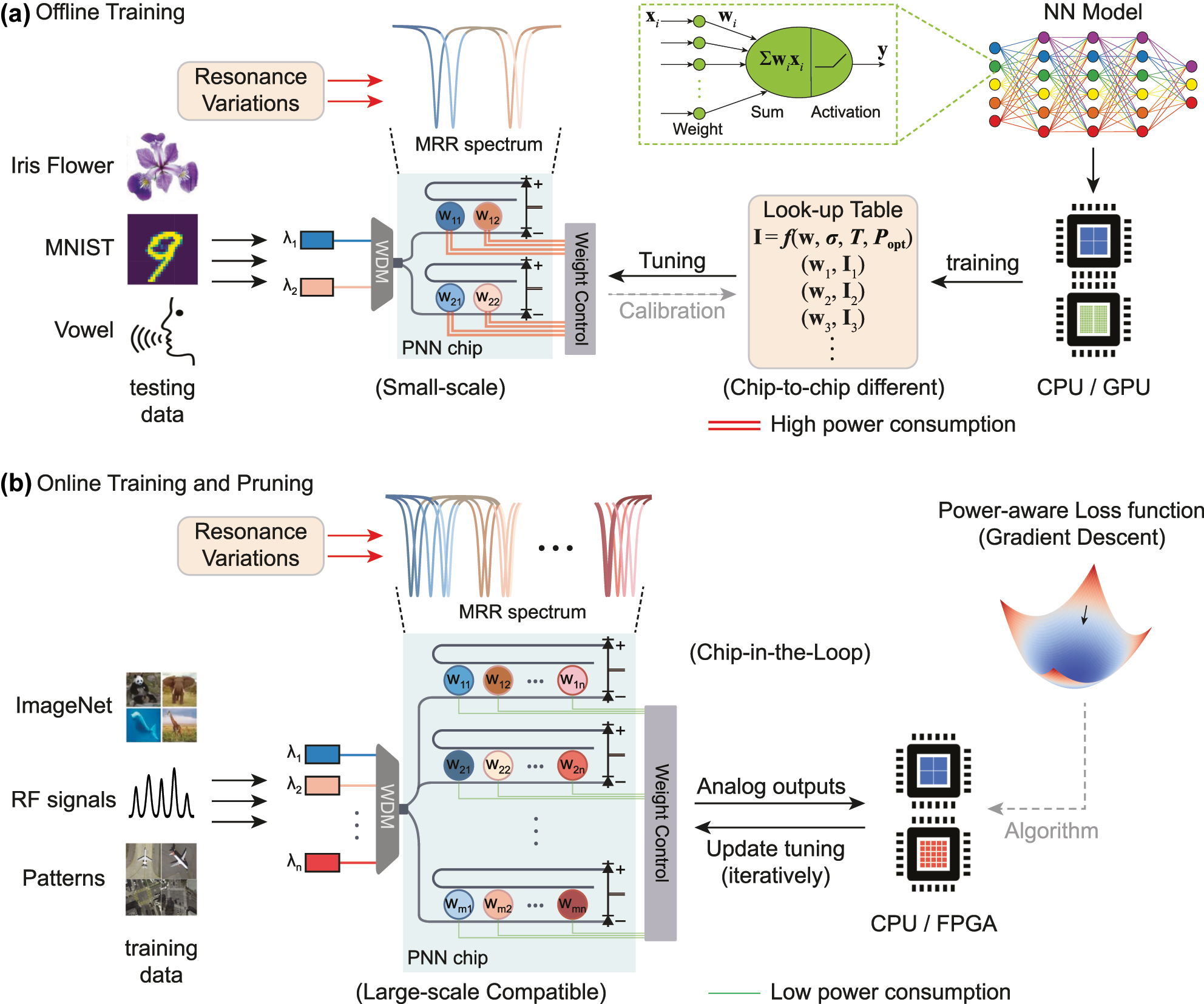
Comparison of offline training with online training and pruning approach. (a) Conventional offline training method supporting only small-scale PNN chips. In this approach, NN parameters are calculated in software and mapped onto the PNN chips. The resonance variations of MRRs necessitate complicated look-up tables, and lead to higher power consumption for MRR control. (b) Online training and pruning method compatible for large-scale PNN chips. The training of PNNs occurs on the same chip used for inference, accounting for any chip-to-chip variations and environmental fluctuations. Our approach simultaneously optimizes the PNN accuracy and the total power consumption for tuning all the MRRs.

Here w _ij denotes the weight to be executed on the i, jth MRR, and I _ij is the required tuning current. The LUT, denoted as a mapping function f _ij , is determined by the relative position of the jth laser wavelength and the MRR resonant state. Ideally, the MRRs operating at the same laser wavelength are expected to exhibit identical resonant wavelengths, simplifying the LUT to f _j .

However, in practice, the MRRs in the same column may exhibit significantly different resonant wavelengths due to static and dynamic variations. As derived in Supplementary Note 1, an LUT for the i, jth MRR – accounting for FPVs, ambient temperature variations, input optical power, and the self-heating effect – is approximately given by

where σ _ij denotes the deviation of resonant wavelength due to FPVs, T is the time-varying ambient temperature, P_opt is the input optical power. Based on Eq. (5), it remains complicated to generate an LUT that accounts for all the non-idealities across large-scale MRR weight banks. Any inaccuracies in LUTs will directly introduce arbitrary deviations in the mapped weight parameters, leading to significant performance degradation across NN system benchmarks such as classification tasks.

In an MRR-based weight bank using thermo-optic tuning to counteract these non-idealities, the required electrical power for actively programming weights of the i, jth MRR can be written as [24]:

where R is the resistance of the metal heater. The power breaks down into a static weight locking power that locks the MRR resonance to the desired wavelength, and a configuration power to program the weight value [24]. Therefore, the total power for the weight configuration consumed by an M × N MRR weight bank is

For simplicity, we denote P^weight as P in the following sections except Section 2.3.

2.1.2 Online training

Online training, also known as “in situ” or “chip-in-the-loop” training, was originally proposed to alleviate the intensive use required of CPU/GPUs for training non Von-Neumann architecture based computing hardware [44], where the training occurs on the same hardware used for inference. It was also recognized that online training can mitigate hardware nonidealities, and promise for iterative weight updates in real-time [45]. The state-of-the-art online training algorithms for PNNs [6], [45], [46], [47], [48] can be classified into two major categories: gradient-based and gradient-free algorithms. Gradient-free algorithms, such as genetic algorithms [47], are straightforward to implement in practice but often face inherent challenges with convergence and scalability. In contrast, gradient-based algorithms are typically more efficient and, therefore, more widely adopted. The most commonly used gradient-based training algorithm for software-based NNs, backpropagation, analytically computes gradients by back-propagating errors using the chain rule [37]. While significant progress has been made in experimentally realizing BP on photonic hardware [48], [49], [50], the process typically requires global optical power monitoring and evaluation of nonlinear activation function gradients in software. This approach introduces additional system complexity and latency overhead. Other gradient-based algorithms, such as direct feedback alignment [45], replace the chain rule in back-propagation with a random weight matrix, but their validation has been limited to small, shallow NNs.

In our approach, the online training of our MRR-based PNNs is implemented by a perturbation-based gradient descent algorithm, which estimates gradients only based on forward inference running on PNN chips. Here, the NN parameters to be optimized are set to be MRR tuning currents instead of neuron weights:

The gradient of loss function with respect to MRR tuning currents (I ^k ) is approximately given by perturbation measurement:

where ΔI ^k is the perturbation rate of the MRR tuning currents in the kth training epoch, and Δ L is the measured change of loss function induced by the perturbation. In practice, ΔI ^k should be sufficiently small to preserve the validity of approximation in Eq. (9), while remaining large enough to produce measurable Δ L above experimental noise.

2.1.3 Pruning

In software-based NNs, pruning is a model compression technique that removes redundant weight parameters (by setting their values to zero) whilst maintaining accuracy. While the implementation of pruning has also been investigated in PNNs, prior approaches either lack robustness against nonidealities [51], [52] or require extensive offline training [26]. As shown in Figure 1b, our proposed approach accounts for the total MRR tuning power in the “chip-in-the-loop” process, by incorporating a power-aware “pruning” term into the conventional loss function:

where L ̃ is the modified loss function given by the sum of the conventional loss function L and the power-aware pruning term γP, γ is an empirically determined hyperparameter that defines pruning strength. According to Eqs. (6) and (7), L ̃ can also be expressed as

The selection of the hyperparameter γ is critical in this framework, as it explicitly parameterizes the trade-off between the NN accuracy and energy efficiency. Depending on the demand of the end users, minimizing this modified loss function can enable concurrent optimization of both the NN accuracy and the total power consumption. For example, in a power-constrained environment, the training problem becomes

with a relatively larger value of γ, where P_max denotes the maximum power available for weight configurations. Oppositely, in scenarios prioritizing high accuracies, it becomes

with a relatively smaller value of γ, where L max denotes the upper bound of the conventional loss function permitted under a given accuracy constraint.

2.2.1 Setup

Recently, integrated PNNs have been extensively investigated and experimentally validated across various on-chip scales, achieving low latencies of hundreds of picoseconds at diverse applications [6], [41], [53]. Notable demonstrations include a 3-layer PNN with 9 neurons for image classification [53], a 3-layer 6 × 6 PNN for vowel classification task [6], and a single-layer 4 × 2 PNN for fiber nonlinearity compensation [40]. In our proof-of-concept experiment, a 3 × 2 MRR weight bank is used to demonstrate our proposed online training and pruning approach and the associated energy savings.

Our experimental setup is illustrated in Figure 2a. First, three channels of input data (denoted as x₁, x₂, x₃) are generated from a high sampling rate signal generator (Keysight M8196A), and modulated onto laser 1, 2, and 3 (Pure-Photonics, PPCL500) respectively via Mach–Zehnder modulators (MZMs). The lights from these three lasers, each at a distinct wavelength, are combined using a wavelength-division multiplexer (MUX) and then split equally between two MRR weight banks. Each MRR weight bank consists of three MRRs, which are designed with slightly different radii (8 μm, 8.012 μm, 8.024 μm). The MRRs at the same column (i.e., MRR1 and MRR4, MRR2 and MRR5, MRR3 and MRR6) are expected to share the same corresponding resonance wavelengths, aligned with 200 GHz spaced ITU grids (1,546.92 nm, 1,548.51 nm, 1,550.12 nm, respectively). However, as shown in Figure 2b, the measured weight bank spectrum indicates that the resonance wavelengths of all six MRRs deviate from the designed values due to FPVs and temperature changes. To counteract FPVs, the wavelengths of three lasers are further tuned (1,547.24 nm, 1,548.60 nm, and 1,550.40 nm) to align with the deviated resonance wavelengths. Moreover, all MRRs are thermally tuned via embedded N-doped heaters to actively program and configure weights (denoted as w₁₁, w₁₂, w₁₃, w₂₁, w₂₂, w₂₃), allowing for individual weighting of input analog data in the three wavelength channels. The thermal tuning characteristics of six MRRs at 30 °C, are illustrated in Figure 2c.

Figure 2:

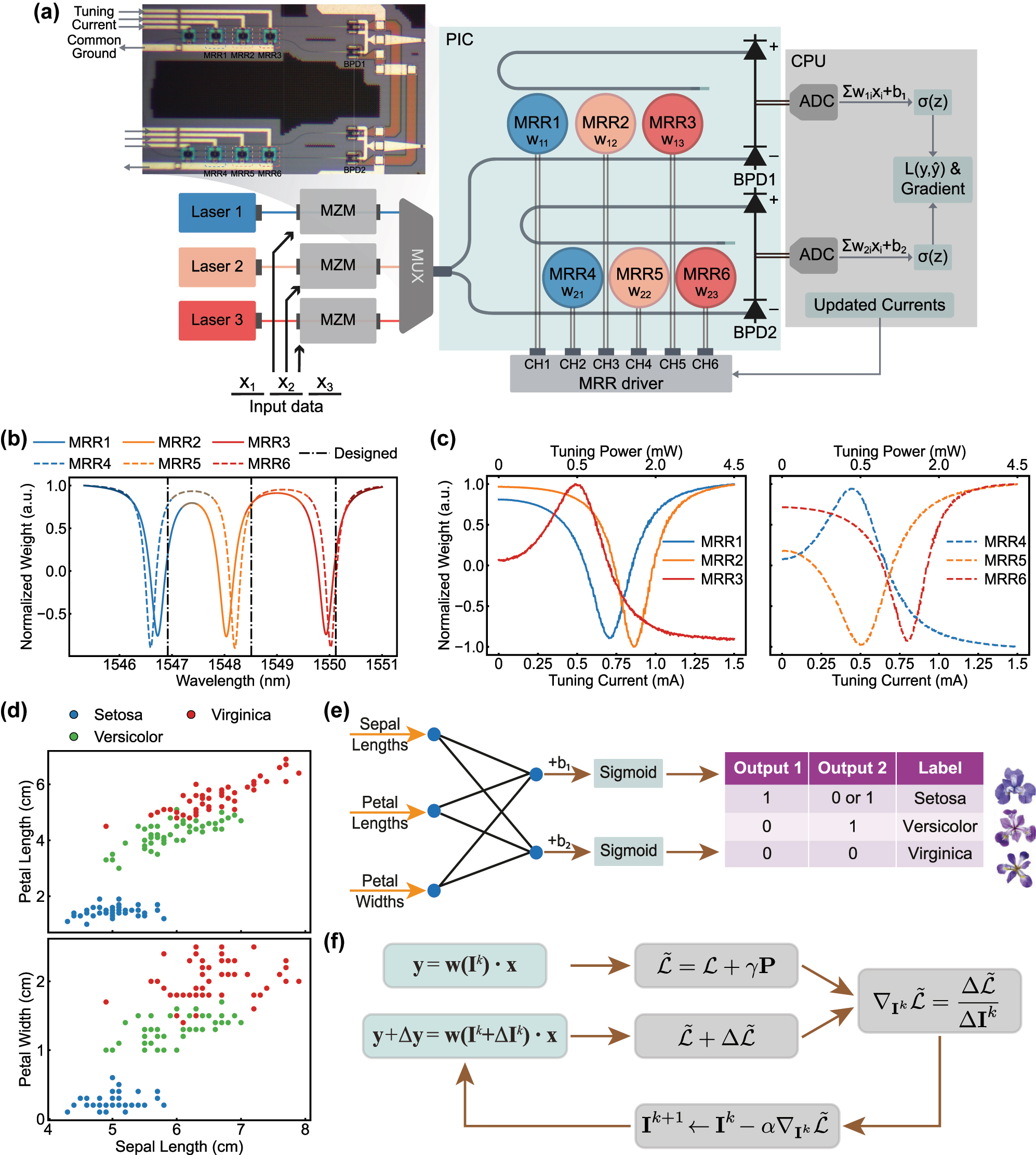
System setup of online training and pruning. (a) Schematic of our experimental setup. MZM, Mach–Zehnder modulator. MUX, wavelength multiplexer. PIC, photonic integrated circuit. MRR, microring resonator. BPD, balanced photodetector. ADC, analog-to-digital converter. CPU, central processing unit. σ(z) denotes the nonlinear activation function performed on software. The inset shows the micrograph of the two MRR weight banks and BPDs. (b) Normalized weight spectrum of two MRR weight banks at 30 °C. The MRRs at the same colors (i.e., MRR1 and MRR4, MRR2 and MRR5, MRR3 and MRR6) are designed to share the same resonance wavelengths, aligned with 200 GHz spaced ITU grids (1,546.92 nm, 1,548.51 nm, 1,550.12 nm). (c) Tuning characteristics of six MRRs at 30 °C. (d) Scatterplot of Iris flower dataset. (e) Schematic of a simple 3 × 2 neural network for Iris classification. (f) Online training and pruning procedure. At each iteration, the PIC performs matrix-vector multiplication without and with perturbations, while the CPU evaluates the gradients of power-aware loss function, and updates the MRR tuning currents for the next iteration.

Our proof-of-concept experiment is validated on a standard Iris dataset, where three species of Iris flowers (Setosa, Versicolour, Virginica) are classified using only three out of four input features (sepal length, petal length, and petal width), as shown in Figure 2d. This three-class classification problem is converted into a two-step binary classification (Figure 2e) mapped to the on-chip PNN, which utilizes eight trainable parameters. The parameters include the tuning currents of six MRRs – I₁₁, I₁₂, I₁₃, I₂₁, I₂₂, I₂₃ (corresponding to six weights) – and two biases, b₁ and b₂. The 150 samples are split into 120 for training and 30 for testing.

The analog optical signals from the drop and through port are then captured and differentiated by two balanced photodetectors (BPDs), which gives the electrical output of the weighted summations, Σ _i w_1ix _i and Σ _i w_2ix _i . The output is further read by an oscilloscope and demodulated in a CPU, which evaluates the power-aware loss function (Eq. (10)) and calculates gradients based on perturbation (Eq. (9)). Finally, the CPU updates the MRR tuning currents for the next training epoch (Eq. (8)) and commands the MRR driver, which is equipped on a customized printed circuit board (PCB) (Supplementary Note 2). As shown in Figure 2f, the training of our PNN occurs with the photonic chip in the loop, iteratively optimizing the loss function and reducing the total power consumption.

2.2.2 Demonstration on 3 × 2 PNN

PNN training is conducted under three conditions: conventional offline training, online training without pruning, and online training with pruning. Each training configuration is repeated 10 times to ensure consistency. The perturbation rate of MRR tuning currents (ΔI ^k ) is set to 0.05 mA. To evaluate the gradients with respect to the MRR tuning currents ∇ I k L , each training epoch batches the training data seven times through the PNN: six times perturbing each tuning current I i j k + Δ I i j k and one time to measure L ̃ with non-perturbed currents I i j k . The plots in Figure 3a show the average of both categorical cross-entropy loss ( L ) and power-aware loss ( L ̃ ) versus training epoch. It is observed that the PNN can quickly converge to the optimal weights within 25 epochs using perturbation-based online training.

Figure 3:

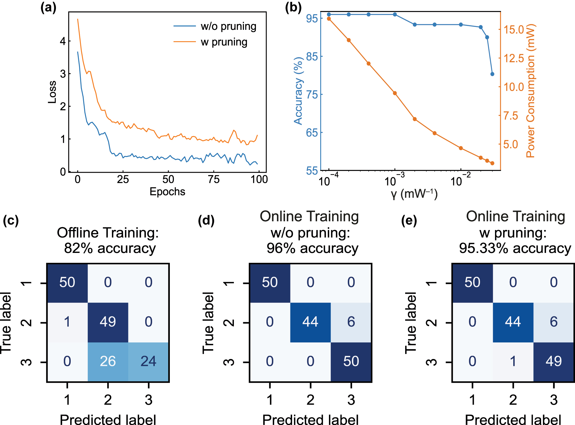
Online training results without, or with pruning method. (a) Experimental results of online training losses without, or with the pruning method. (b) Simulated result indicating the tradeoff between the prediction accuracy and power efficiency. (c–e) Confusion matrices for the 150 samples, obtained by the conventional offline training, online training without, or with the pruning method, respectively.

We also simulate the trade-off between the NN accuracy and the associated energy savings (Figure 3b). The simulation indicates that the trade-off is optimized at γ_opt = 0.01 mW⁻¹, where significant reduction of overall tuning power (exceeding 70 %) can be achieved before the accuracy drops off. As predicted in Section 2.1.3, in scenarios prioritizing high accuracies where γ < γ_opt, the loss function L ̃ is dominated by the conventional loss function L , such that the PNN maintains a high accuracy of >93 %. Contrarily, in scenarios constraining overall power consumption where γ > γ_opt, the power-aware loss function L ̃ is dominated by the pruning term γP, leading to a larger amount of energy savings but may degrade the PNN accuracy. As shown by the confusion matrix in Figure 3c, the offline training experiment only produces 82 % accuracy on the 150 samples. In the accuracy-prioritized online training experiment (without pruning, γ set to 0) (Figure 3d), the overall classification of the Iris flower task is improved to 96 %, with a total MRR tuning power of 9.54 mW. In the online training experiment constraining power consumption (with pruning, γ set to 0.0075 mW⁻¹) (Figure 3e), we observe a 44.7 % reduction (from 9.54 mW to 5.28 mW) of total tuning power while the PNN maintains a classification accuracy of 95.33 %.

Furthermore, to demonstrate the adaptability of our online training method to temperature drifts, additional experiments are conducted at multiple different temperatures ranging from 26 °C to 40 °C. Before online training, the MRR tuning currents are randomly initialized within the tuning range of 0–1.5 mA (only weights w₁₁ and w₂₁ are plotted, Figure 4a), producing untrained classification outputs with only 33.33 % accuracy. After online training for 100 epochs (Figure 4b), the PNN can be trained to the optimal weights, regardless of the changes of MRR tuning characteristics due to temperature drifts. As a result, high classification accuracies is consistently achieved at both 30 °C (99.33 %, upper row of Figure 4a and b) and 34 °C (96.67 %, lower row of Figure 4a and b). As shown in Figure 4c, the classification accuracies maintain above 90 % even if the external temperature changes from 26 °C to 40 °C. We also evaluate the resilience of our PNN training to intentional thermal disturbances. In Figure 4d, it is shown that the PNN can quickly recover its classification performance within about 25 epochs even if the external temperature is disturbed from 27 °C to 32 °C (at the 100th epoch), and from 32 °C to 30 °C (at the 200th epoch). These proof-of-concept experimental results further confirm that our online training and pruning method can handle any PNN hardware non-idealities, including chip-to-chip FPVs, temperature disturbances, and even nonlinearities induced by input optical power.

Figure 4:

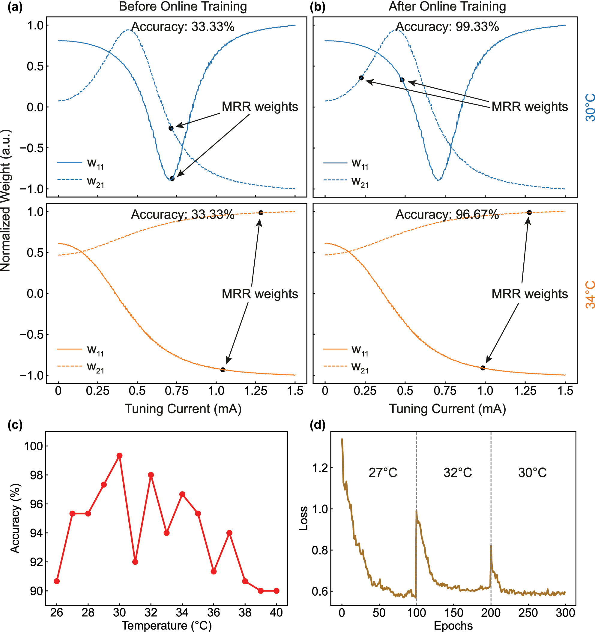
Adaptive PNN training at different temperatures. (a, b) Illustrate two of the six MRR tuning currents (weights I₁₁ and I₂₁) before and after online training, respectively, at 30 °C (the upper plots) and 34 °C (the lower plots). (c) Experimental obtained Iris classification accuracies at different temperatures. (d) Online training experiment performed with thermal disturbances. The temperature is changed from 27 °C to 32 °C at the 100th epoch, and from 32 °C to 30 °C at the 200th epoch.

References

[1] J. Chen and X. Ran, “Deep learning with edge computing: a review,” Proc. IEEE, vol. 107, no. 8, pp. 1655–1674, 2019, https://doi.org/10.1109/jproc.2019.2921977.Suche in Google Scholar
[2] L. Ouyang et al.., “Training language models to follow instructions with human feedback,” in Advances in Neural Information Processing Systems, vol. 35, 2022, pp. 27730–27744.Suche in Google Scholar
[3] Y. LeCun, Y. Bengio, and G. Hinton, “Deep learning,” Nature, vol. 521, no. 7553, pp. 436–444, 2015, https://doi.org/10.1038/nature14539.Suche in Google Scholar PubMed
[4] Y. Shen et al.., “Deep learning with coherent nanophotonic circuits,” Nat. Photonics, vol. 11, no. 7, pp. 441–446, 2017, https://doi.org/10.1038/nphoton.2017.93.Suche in Google Scholar
[5] B. J. Shastri et al.., “Photonics for artificial intelligence and neuromorphic computing,” Nat. Photonics, vol. 15, no. 2, pp. 102–114, 2021, https://doi.org/10.1038/s41566-020-00754-y.Suche in Google Scholar
[6] S. Bandyopadhyay et al.., “Single-chip photonic deep neural network with forward-only training,” Nat. Photonics, vol. 18, no. 12, pp. 1335–1343, 2024, https://doi.org/10.1038/s41566-024-01567-z.Suche in Google Scholar
[7] Y. Chen et al.., “All-analog photoelectronic chip for high-speed vision tasks,” Nature, vol. 623, no. 7985, pp. 48–57, 2023, https://doi.org/10.1038/s41586-023-06558-8.Suche in Google Scholar PubMed PubMed Central
[8] A. N. Tait et al.., “Neuromorphic photonic networks using silicon photonic weight banks,” Sci. Rep., vol. 7, no. 1, p. 7430, 2017, https://doi.org/10.1038/s41598-017-07754-z.Suche in Google Scholar PubMed PubMed Central
[9] J. Feldmann et al.., “Parallel convolutional processing using an integrated photonic tensor core,” Nature, vol. 589, no. 7840, pp. 52–58, 2021, https://doi.org/10.1038/s41586-020-03070-1.Suche in Google Scholar PubMed
[10] J. C. Lederman et al.., “Low-latency passive thermal desensitization of a silicon micro-ring resonator with self-heating,” APL Photonics, vol. 9, no. 7, p. 076117, 2024, https://doi.org/10.1063/5.0212591.Suche in Google Scholar
[11] S. Y. Siew et al.., “Review of silicon photonics technology and platform development,” J. Lightwave Technol., vol. 39, no. 13, pp. 4374–4389, 2021, https://doi.org/10.1109/jlt.2021.3066203.Suche in Google Scholar
[12] K. Giewont et al.., “300-mm monolithic silicon photonics foundry technology,” IEEE J. Sel. Top. Quantum Electron., vol. 25, no. 5, p. 8200611, 2019.10.1109/JSTQE.2019.2908790Suche in Google Scholar
[13] L. Chrostowski et al.., “Silicon photonic circuit design using rapid prototyping foundry process design kits,” IEEE J. Sel. Top. Quantum Electron., vol. 25, no. 5, p. 8201326, 2019, https://doi.org/10.1109/jstqe.2019.2917501.Suche in Google Scholar
[14] C. Huang et al.., “Prospects and applications of photonic neural networks,” Adv. Phys. X, vol. 7, no. 1, p. 1981155, 2022, https://doi.org/10.1080/23746149.2021.1981155.Suche in Google Scholar
[15] H. Jayatilleka, H. Shoman, L. Chrostowski, and S. Shekhar, “Photoconductive heaters enable control of large-scale silicon photonic ring resonator circuits,” Optica, vol. 6, no. 1, pp. 84–91, 2019, https://doi.org/10.1364/optica.6.000084.Suche in Google Scholar
[16] H. Larocque et al.., “Beam steering with ultracompact and low-power silicon resonator phase shifters,” Opt. Express, vol. 27, no. 24, pp. 34639–34654, 2019, https://doi.org/10.1364/oe.27.034639.Suche in Google Scholar
[17] L. Huang et al.., “Integrated light sources based on micro-ring resonators for chip-based LiDAR,” Laser Photonics Rev., vol. 19, no. 2, p. 2400343, 2025, https://doi.org/10.1002/lpor.202400343.Suche in Google Scholar
[18] M. Nichols, H. Morison, A. Eshaghi, B. Shastri, and L. Lampe, “Photonics-based fully-connected hybrid beamforming: towards scaling up massive MIMO at higher frequency bands,” Res. Sq., 2024. https://doi.org/10.21203/rs.3.rs-4627859/v1.Suche in Google Scholar
[19] Y. Liu et al.., “Ultra-low-loss silicon nitride optical beamforming network for wideband wireless applications,” IEEE J. Sel. Top. Quantum Electron., vol. 24, no. 4, p. 8300410, 2018, https://doi.org/10.1109/jstqe.2018.2827786.Suche in Google Scholar
[20] A. Rizzo et al.., “Massively scalable Kerr comb-driven silicon photonic link,” Nat. Photonics, vol. 17, no. 9, pp. 781–790, 2023, https://doi.org/10.1038/s41566-023-01244-7.Suche in Google Scholar
[21] S. Daudlin, et al.., “Three-dimensional photonic integration for ultra-low-energy, high-bandwidth interchip data links,” Nat. Photonics, vol. 19, no. 5, pp. 502–509, 2025. https://doi.org/10.1038/s41566-025-01633-0.Suche in Google Scholar
[22] W. Bogaerts et al.., “Silicon microring resonators,” Laser Photonics Rev., vol. 6, no. 1, pp. 47–73, 2012, https://doi.org/10.1002/lpor.201100017.Suche in Google Scholar
[23] A. Densmore et al.., “A silicon-on-insulator photonic wire based evanescent field sensor,” IEEE Photonics Technol. Lett., vol. 18, no. 23, pp. 2520–2522, 2006, https://doi.org/10.1109/lpt.2006.887374.Suche in Google Scholar
[24] A. N. Tait, “Quantifying power in silicon photonic neural networks,” Phys. Rev. Appl., vol. 17, no. 5, p. 054029, 2022, https://doi.org/10.1103/physrevapplied.17.054029.Suche in Google Scholar
[25] L. Chrostowski, X. Wang, J. Flueckiger, Y. Wu, Y. Wang, and S. T. Fard, “Impact of fabrication non-uniformity on chip-scale silicon photonic integrated circuits,” in Optical Fiber Communication Conference, 2014, pp. 2–37.10.1364/OFC.2014.Th2A.37Suche in Google Scholar
[26] T. Xu et al.., “Control-free and efficient integrated photonic neural networks via hardware-aware training and pruning,” Optica, vol. 11, no. 8, pp. 1039–1049, 2024, https://doi.org/10.1364/optica.523225.Suche in Google Scholar
[27] M. M. Milosevic et al.., “Ion implantation in silicon for trimming the operating wavelength of ring resonators,” IEEE J. Sel. Top. Quantum Electron., vol. 24, no. 4, p. 8200107, 2018, https://doi.org/10.1109/jstqe.2018.2799660.Suche in Google Scholar
[28] B. Chen et al.., “Real-time monitoring and gradient feedback enable accurate trimming of ion-implanted silicon photonic devices,” Opt. Express, vol. 26, no. 19, pp. 24953–24963, 2018, https://doi.org/10.1364/oe.26.024953.Suche in Google Scholar PubMed
[29] C. Ríos et al.., “Integrated all-photonic non-volatile multi-level memory,” Nat. Photonics, vol. 9, no. 11, pp. 725–732, 2015, https://doi.org/10.1038/nphoton.2015.182.Suche in Google Scholar
[30] Z. Fang et al.., “Ultra-low-energy programmable non-volatile silicon photonics based on phase-change materials with graphene heaters,” Nat. Nanotechnol., vol. 17, no. 8, pp. 842–848, 2022, https://doi.org/10.1038/s41565-022-01153-w.Suche in Google Scholar PubMed
[31] J. Zheng et al.., “GST-on-silicon hybrid nanophotonic integrated circuits: a non-volatile quasi-continuously reprogrammable platform,” Opt. Mater. Express, vol. 8, no. 6, pp. 1551–1561, 2018, https://doi.org/10.1364/ome.8.001551.Suche in Google Scholar
[32] X. Yang et al.., “Non-volatile optical switch element enabled by low-loss phase change material,” Adv. Funct. Mater., vol. 33, no. 42, p. 2304601, 2023, https://doi.org/10.1002/adfm.202304601.Suche in Google Scholar
[33] S. Bilodeau et al.., “All-optical organic photochemical integrated nanophotonic memory: low-loss, continuously tunable, non-volatile,” Optica, vol. 11, no. 9, pp. 1242–1249, 2024, https://doi.org/10.1364/optica.529336.Suche in Google Scholar
[34] L. Xu et al.., “Building scalable silicon microring resonator-based neuromorphic photonic circuits using post-fabrication processing with photochromic material,” Adv. Opt. Mater., vol. 13, no. 11, p. 2402706, 2025, https://doi.org/10.1002/adom.202402706.Suche in Google Scholar
[35] H. Jayatilleka et al.., “Wavelength tuning and stabilization of microring-based filters using silicon in-resonator photoconductive heaters,” Opt. Express, vol. 23, no. 19, pp. 25084–25097, 2015, https://doi.org/10.1364/oe.23.025084.Suche in Google Scholar PubMed
[36] C. Huang et al.., “Demonstration of scalable microring weight bank control for large-scale photonic integrated circuits,” APL Photonics, vol. 5, no. 4, p. 040803, 2020, https://doi.org/10.1063/1.5144121.Suche in Google Scholar
[37] Y. LeCun, L. Bottou, Y. Bengio, and P. Haffner, “Gradient-based learning applied to document recognition,” Proc. IEEE, vol. 86, no. 11, pp. 2278–2324, 1998, https://doi.org/10.1109/5.726791.Suche in Google Scholar
[38] A. Krizhevsky and G. Hinton, “Learning multiple layers of features from tiny images,” Tech. Rep., 2009. Available at: https://www.cs.utoronto.ca/∼kriz/learning-features-2009-TR.pdf.Suche in Google Scholar
[39] H. Xiao, K. Rasul, and R. Vollgraf, “Fashion-MNIST: a novel image dataset for benchmarking machine learning algorithms,” arXiv preprint arXiv:1708.07747, 2017.Suche in Google Scholar
[40] C. Huang et al.., “A silicon photonic–electronic neural network for fibre nonlinearity compensation,” Nat. Electron., vol. 4, no. 11, pp. 837–844, 2021, https://doi.org/10.1038/s41928-021-00661-2.Suche in Google Scholar
[41] W. Zhang et al.., “A system-on-chip microwave photonic processor solves dynamic RF interference in real time with picosecond latency,” Light: Sci. Appl., vol. 13, no. 1, p. 14, 2024, https://doi.org/10.1038/s41377-023-01362-5.Suche in Google Scholar PubMed PubMed Central
[42] X. Zhou, D. Yi, D. W. U. Chan, and H. K. Tsang, “Silicon photonics for high-speed communications and photonic signal processing,” npj Nanophoton., vol. 1, no. 1, p. 27, 2024, https://doi.org/10.1038/s44310-024-00024-7.Suche in Google Scholar
[43] X. Lin et al.., “All-optical machine learning using diffractive deep neural networks,” Science, vol. 361, no. 6406, pp. 1004–1008, 2018, https://doi.org/10.1126/science.aat8084.Suche in Google Scholar PubMed
[44] S. M. Buckley, A. N. Tait, A. N. McCaughan, and B. J. Shastri, “Photonic online learning: a perspective,” Nanophotonics, vol. 12, no. 5, pp. 833–845, 2023, https://doi.org/10.1515/nanoph-2022-0553.Suche in Google Scholar PubMed PubMed Central
[45] M. J. Filipovich et al.., “Silicon photonic architecture for training deep neural networks with direct feedback alignment,” Optica, vol. 9, no. 12, pp. 1323–1332, 2022, https://doi.org/10.1364/optica.475493.Suche in Google Scholar
[46] T. W. Hughes, M. Minkov, Y. Shi, and S. Fan, “Training of photonic neural networks through in situ backpropagation and gradient measurement,” Optica, vol. 5, no. 7, pp. 864–871, 2018, https://doi.org/10.1364/optica.5.000864.Suche in Google Scholar
[47] H. Zhang et al.., “Efficient on-chip training of optical neural networks using genetic algorithm,” ACS Photonics, vol. 8, no. 6, pp. 1662–1672, 2021, https://doi.org/10.1021/acsphotonics.1c00035.Suche in Google Scholar
[48] S. Pai et al.., “Experimentally realized in situ backpropagation for deep learning in photonic neural networks,” Science, vol. 380, no. 6643, pp. 398–404, 2023, https://doi.org/10.1126/science.ade8450.Suche in Google Scholar PubMed
[49] M. Hermans, M. Burm, T. Van Vaerenbergh, J. Dambre, and P. Bienstman, “Trainable hardware for dynamical computing using error backpropagation through physical media,” Nat. Commun., vol. 6, no. 1, p. 6729, 2015, https://doi.org/10.1038/ncomms7729.Suche in Google Scholar PubMed PubMed Central
[50] Z. Gu, Z. Huang, Y. Gao, and X. Liu, “Training optronic convolutional neural networks on an optical system through backpropagation algorithms,” Opt. Express, vol. 30, no. 11, pp. 19416–19440, 2022, https://doi.org/10.1364/oe.456003.Suche in Google Scholar
[51] S. Banerjee, M. Nikdast, S. Pasricha, and K. Chakrabarty, “Pruning coherent integrated photonic neural networks,” IEEE J. Sel. Top. Quantum Electron., vol. 29, no. 2, p. 6101013, 2023, https://doi.org/10.1109/jstqe.2023.3242992.Suche in Google Scholar
[52] J. Gu, C. Feng, Z. Zhao, Z. Ying, R. T. Chen, and D. Z. Pan, “Efficient on-chip learning for optical neural networks through power-aware sparse zeroth-order optimization,” Proc. AAAI Conf. Artif. Intell., vol. 35, no. 9, pp. 7583–7591, 2021, https://doi.org/10.1609/aaai.v35i9.16928.Suche in Google Scholar
[53] F. Ashtiani, A. J. Geers, and F. Aflatouni, “An on-chip photonic deep neural network for image classification,” Nature, vol. 606, no. 7914, pp. 501–506, 2022, https://doi.org/10.1038/s41586-022-04714-0.Suche in Google Scholar PubMed
[54] E. Timurdogan, C. M. Sorace-Agaskar, J. Sun, E. Shah Hosseini, A. Biberman, and M. R. Watts, “An ultralow power athermal silicon modulator,” Nat. Commun., vol. 5, no. 1, pp. 1–11, 2014, https://doi.org/10.1038/ncomms5008.Suche in Google Scholar PubMed PubMed Central
[55] Y. Xiang, H. Cao, C. Liu, J. Guo, and D. Dai, “High-speed waveguide Ge/Si avalanche photodiode with a gain-bandwidth product of 615 GHz,” Optica, vol. 9, no. 7, pp. 762–769, 2022, https://doi.org/10.1364/optica.462609.Suche in Google Scholar
[56] Z. Xu, T. Zhou, M. Ma, C. Deng, Q. Dai, and L. Fang, “Large-scale photonic chiplet Taichi empowers 160-TOPS/W artificial general intelligence,” Science, vol. 384, no. 6692, pp. 202–209, 2024, https://doi.org/10.1126/science.adl1203.Suche in Google Scholar PubMed
[57] Z. Xue, T. Zhou, Z. Xu, S. Yu, Q. Dai, and L. Fang, “Fully forward mode training for optical neural networks,” Nature, vol. 632, no. 8024, pp. 280–286, 2024, https://doi.org/10.1038/s41586-024-07687-4.Suche in Google Scholar PubMed PubMed Central
[58] T. Zhou et al.., “Large-scale neuromorphic optoelectronic computing with a reconfigurable diffractive processing unit,” Nat. Photonics, vol. 15, no. 5, pp. 367–373, 2021, https://doi.org/10.1038/s41566-021-00796-w.Suche in Google Scholar
[59] A. N. McCaughan, B. G. Oripov, N. Ganesh, S. W. Nam, A. Dienstfrey, and S. M. Buckley, “Multiplexed gradient descent: fast online training of modern datasets on hardware neural networks without backpropagation,” APL Mach. Learn., vol. 1, no. 2, p. 026118, 2023, https://doi.org/10.1063/5.0157645.Suche in Google Scholar
[60] D. W. Chan, X. Wu, Z. Zhang, C. Lu, A. P. T. Lau, and H. K. Tsang, “Ultra-wide free-spectral-range silicon microring modulator for high capacity WDM,” J. Lightwave Technol., vol. 40, no. 24, pp. 7848–7855, 2022, https://doi.org/10.1109/jlt.2022.3208745.Suche in Google Scholar
[61] Y. Yuan et al.., “A 5 × 200 Gbps microring modulator silicon chip empowered by two-segment Z-shape junctions,” Nat. Commun., vol. 15, no. 1, p. 918, 2024, https://doi.org/10.1038/s41467-024-45301-3.Suche in Google Scholar PubMed PubMed Central
Supplementary Material
This article contains supplementary material (https://doi.org/10.1515/nanoph-2025-0296).
© 2025 the author(s), published by De Gruyter, Berlin/Boston
This work is licensed under the Creative Commons Attribution 4.0 International License.
Artikel in diesem Heft
- Frontmatter
- Reviews
- Light-driven micro/nanobots
- Tunable BIC metamaterials with Dirac semimetals
- Large-scale silicon photonics switches for AI/ML interconnections based on a 300-mm CMOS pilot line
- Perspective
- Density-functional tight binding meets Maxwell: unraveling the mysteries of (strong) light–matter coupling efficiently
- Letters
- Broadband on-chip spectral sensing via directly integrated narrowband plasmonic filters for computational multispectral imaging
- Sub-100 nm manipulation of blue light over a large field of view using Si nanolens array
- Tunable bound states in the continuum through hybridization of 1D and 2D metasurfaces
- Integrated array of coupled exciton–polariton condensates
- Disentangling the absorption lineshape of methylene blue for nanocavity strong coupling
- Research Articles
- Demonstration of multiple-wavelength-band photonic integrated circuits using a silicon and silicon nitride 2.5D integration method
- Inverse-designed gyrotropic scatterers for non-reciprocal analog computing
- Highly sensitive broadband photodetector based on PtSe2 photothermal effect and fiber harmonic Vernier effect