Neutrosophic Inventory Management: A Cost-Effective Approach
-
Ankit Dubey


Abstract
Classical inventory models (IM) serve as quantitative tools for determining the optimal order quantities, timing of orders, and safety stock levels for specific inventory items or item groups. Zadeh (1965. Fuzzy sets. Information and Control, 8, 338–353) introduced fuzzy theory and Dubois and Parade (1988. Fuzzy logic in expert systems: The role of uncertainty management. Fuzzy Sets and Systems, 28, 3–17) presented the study of fuzzy inventory model, which, however, exhibits limitations in effectively handling uncertainty, inaccuracies, and imprecise data. In 1999, Smarandache presented the idea of neutrosophic set theory to handle uncertainty. Using trapezoidal neutrosophic numbers, this study extends the idea of neutrosophic sets to inventory management, concentrating on resolving the uncertainty associated with holding costs, ordering costs, and shortage costs. First time within the literature of the neutrosophic set, our new method not only addresses existing problems but can also tackle other issues that no other authors have successfully resolved so far. Additionally, we conduct a comparative analysis of our proposed model against existing models in this article. Based on this comparative study, our findings assert the superior performance of our proposed model in relation to some of the existing models. In conclusion, we wrap up our research by presenting graphical, logical, and tabular comparisons with the existing methods.
1 Introduction
Operations research, often abbreviated as OR, is a multidisciplinary field at the intersection of mathematics, statistics, and decision science. The field of OR is incredibly vast and fascinating. It encompasses numerous applications, making it challenging to fully comprehend. As researchers, we have observed that the most significant issue across all these applications is uncertainty, as highlighted in Table 1.
OR at work: exploring the diverse applications across various fields
| S. no. | Authors and year | Uncertain environments | Applications | Significance |
|---|---|---|---|---|
| 1 | Akram et al. (2016) | Bipolar fuzzy | Computing | Bipolar fuzzy digraphs for decision support systems |
| 2 | Butt and Akram (2016b) | Intuitionistic fuzzy | Decision making | A novel decision-making system based on intuitionistic fuzzy rule for an operating system process scheduler |
| 3 | Butt and Akram (2016a) | Fuzzy | CPU scheduling | Enhancing CPU scheduling algorithms using a novel fuzzy decision-making system |
| 4 | Habib et al. (2017) | Fuzzy | Climate decision | Developing fuzzy climate decision support systems for tomato cultivation in high tunnels |
| 5 | Farnam and Darehmiraki (2021) | Hesitant fuzzy | Multi-objective problem | Procedure for solving a multi-objective fractional programming issue in an environment of hesitant fuzzy decision-making |
| 6 | Mohanta and Sharanappa (2024) | Neutrosophic | Data analysis | A thorough review and current trends in neutrosophic data envelopment analysis |
| 7 | Iqbal et al. (2023) | Fermatean probabilistic hesitant fuzzy | Disaster | Enhancing earthquake response using Fermatean probabilistic hesitant fuzzy sets |
| 8 | Edalatpanah (2023) | Fuzzy | LPP | Solving fuzzy LPP in multiple dimensions |
| 9 | Alburaikan et al. (2023) | Neutrosophic | Goal programming | The goal programming approach to solving linear fractional programming problems with multiple objectives is based on a Neutrosophic scenario |
| 10 | Masoomi et al. (2023) | Neutrosophic | Supply chain | An improved best-worst method using Neutrosophic logic for evaluating performance indicators in the renewable energy supply chain |
Now, as we know, our article primarily focuses on IM. Therefore, we have proceeded to discuss IM further. Operations research is intricately connected to inventory management by providing a systematic approach to optimize key inventory decisions. Through mathematical models, simulations, and analysis, operations research enables businesses to determine optimal reorder points, order quantities, and inventory policies, accounting for factors like demand variability, lead times, and cost structures. This connection empowers organizations to minimize holding and ordering costs while maintaining desired service levels, enhancing overall supply chain efficiency and profitability through data-driven decision-making in the realm of inventory management.
The last few years have witnessed a growing body of research focusing on various dimensions of inventory control and management. Numerous studies have explored complex facets with an emphasis on dealing with demand that changes depending on pricing and partial backlog, Das et al. (2020) integrated preservation technology into an inventory control system. In 2020, Mashud contributed by introducing an EOQ framework for a failing IM that considers various forms of demands and full backlog. In the year 2021, Khan and Sarkar investigated the landscape of risk transfer in the supply chain, integrating price and inventory decisions and handling shortages with great care. To tackle difficult inventory control situations, Setiawan et al. (2021) provided helpful information on how to handle exponential and quadratic demand in the context of Weibull deterioration. In the following year, Sharma et al. (2022) published their work, which developed a model that considers demand-driven production and accounts for time and stock-related demand for items with declining inventory. An adaptive IM that is specifically designed for pharmaceutical distribution, with dynamic discreteness and the ability to account for both deterministic and stochastic demand, was presented by Antic et al. (2022). Duary et al. (2022) extended the scope by considering payment timing and inventory discounts in a model for deteriorating items, thoughtfully incorporating capacity constraints and partially backlogged shortages. The most recent addition, by Jani et al. (2023), offers a decision support system tailored for retailer's deterioration control, factoring in trade credit dynamics and the presence of shortages. Farahbakhsh and Kheirkhah (2023) presented a useful genetic algorithm-Taguchi-based method for solving the multi-period inventory route problem. In the same year, Dash et al. (2023) explored the coordination of a single-manufacturer multi-retailer supply chain, taking into account price and green-sensitive demand under stochastic lead time. Miriam et al. (2023) focused on decision-making processes in customer-centric IM. Moving into (2024), Das and Samanta presented an EOQ model for a two-warehouse system during lockdown, considering linear time-dependent demand. Lastly, Nazabadi et al. (2024) using agent-based and reinforcement learning models came up with a joint policy for production, maintenance, and product quality that works for a multi-machine production system. Together, these studies form a comprehensive mosaic of inventory management research, contributing valuable perspectives to this intricate and dynamic field. To avoid stockouts or excess inventory, classical IM must accurately predict future demand to strike a balance between service levels, costs, and reorder points, it must optimize safety stock levels and reorder points etc. In the sun case for a better alternative to classical inventory models (IM), fuzzy logic is useful in situations, where there are numerous complicated factors. In 1965, fuzzy theory was introduced by Lotfi A. Zadeh, which significantly improved its ability to aid in better decision-making.
The fuzzy inventory model (FIM), first proposed by Dubois and Parade (1988), achieves a flexible method of inventory management compared to classical IM. In 2011, Leopoldo Eduardo Cárdenas-Barron used analytical geometry and algebra to create EPQ/EOQ IMs including dual backorder costs. Based on this, Sulak (2015) proposed an EOQ model under a fuzzy set that handled defective shortages and products, offering a more realistic approach to inventory management. In 2019, Gani and colleagues used the AGM inequality approach to determine EOQ/EPQ in a fuzzy situation. This helped with inventory estimations. With a focus on variable holding costs, Alfares and Ghaithan (2019) investigated EOQ and EPQ production-IM, an essential part of contemporary supply chain dynamics. Additional research by Thinakaran et al. (2019) examined partial backorders in EOQ and EPQ IMs. A typical IM issue that may be rather difficult for corporations was shed light on here. To enhance EOQ/EPQ IM formulations with two backorder prices, Lin (2019) utilized algebra and analytic geometry. Gani and Rafi (2020), enhanced EOQ/EPQ calculation using algebraic and AGM inequality approaches to streamline decision-making in a fuzzy context.
Later, Das (2020) introduced the multi-item IM with lead time in his research. In a fuzzy setting, demand influences both production cost and setup cost. In 2022, 2 years after this idea was first proposed, Das further expanded the proposed multi-objective IM in a fuzzy context. In 2022, a new approach was launched to handle production faults in EOQ/EPQ IM with shortages utilizing fuzzy methodologies. This method significantly improved the accuracy and resilience of inventory management. As a group, these academics have tackled many of the challenges and unknowns that contemporary companies confront by making great theoretical and practical advances in the field of inventory management. So far, we have discussed the FIM, but some challenges in FIM. Challenges in FIM involve handling fluctuating demand patterns, addressing imprecise or incomplete data, optimizing inventory allocation and distribution across complex supply chains, and adapting to unforeseen disruptions, whereas extended fuzzy inventory methodologies refine traditional approaches by integrating higher-order fuzzy reasoning, multiple granularities, and dynamic adjustments, enabling more adaptive, resilient, and agile inventory control strategies in volatile and uncertain environments.
However, in 1999, F. Smarandache outlined the neutrosophic set and its unique features that distinguish it apart from the classical and fuzzy models. In the context of this progression, we will now proceed to discuss the neutrosophic inventory model (NIM).
1.1 Motivation and Novelties
Neutrosophic set theory is a technique used for uncertainty in IM. It deals with situations where we’re not entirely sure about something. NIM with Neutrosophic number etc. are described by few researchers. This manuscript's primary contribution is as follows:
The proposed model can address the problems that have already been resolved by existing models.
The proposed model has the capability to address novel problem sets that have not been explored in any existing research article to date.
It reduces the time and space complexity.
1.2 Objective
After reading many research books and articles, it has become clear that having a lot of knowledge about management is very important. Also, it is very important to understand that uncertainty is a big part of real-life problems. Because of these things, the present study aims to explore NIM as a cost-effective approach.
The study aims to explore NIM as a cost-effective approach. To achieve this, the following objectives have been set:
Conducting a comprehensive literature survey on inventory management systems to enhance understanding of the overall management framework.
Proposing a new method to effectively address and manage the neutrosophic within the IM context.
Comparing the proposed method with existing approaches to establish its superiority.
Conducting a thorough comparison, employing logical, graphical, and tabular analyses, with existing methods in the field.
Discussing the practical applications of the proposed method within the inventory management system.
Introducing a new method designed not only to address existing numerical challenges but also to tackle novel problem types.
This research endeavours to contribute to the existing body of knowledge in the field by addressing the identified gaps and offering innovative solutions to enhance the efficacy of IM systems in the face of uncertainty.
The article consists of five sections and Appendix. The first section is the introduction, which provides an overview of the study. The second section presents the proposed NIM Model. The third section is dedicated to numerical analysis with results and discussion. The fourth section presents the sensitive analysis. Finally, the fifth section concludes the article. The appendix contains at first Neutrosophic numbers and their arithmetic and logical operators. at second EOQ model in Neutrosophic environment.
2 Proposed Neutrosophic Inventory Management Model
2.1 Notations
Define the following parameters used in IM:
|
|
|
|
|
|
|
|
|
|
|
|
|
|
|
|
|
|
|
|
|
|
|
|
2.2 Assumptions
This IM allows inventory shortages and constant demand and plan time.
2.3 Mathematical Formation and Solution of Model
2.3.1 EOQ Model in Classical Environment
For a crisp IM with shortage quantity, then IM in the classical sense is,
Total cost = Ordering Cost + Holding Cost + Shortage Cost
where
Now, differentiating equation (1) with respect to
And optimal shortage quantity is
From equation (1), the minimal total cost is
2.3.2 EOQ Model in Neutrosophic Environment
In an environment characterized by its clarity and precision, we can determine the total cost using equation (1). However, in real-world scenarios, this cost may exhibit slight fluctuations, thereby impacting the quantity ordering (
2.3.3 Proposed Model for Find Total Cost while Considering the Uncertainty
The neutrosophic total cost, optimal order quantity, and optimal shortage quantity are denoted as
The optimal order quantity (
The optimal shortage quantity (
Therefore, optimal (minimum) total cost while considering uncertainty is as follows (Appendix B equation (A7)):
3 Numerical Analysis and Result Discussion
The purpose of introducing this section is to explain the validation of our proposed model. Additionally, we have attempted to compare our proposed model with some of the existing models. This comparison helps demonstrate the superiority of our proposed model, and we have used two examples to illustrate this. Specifically, we conducted two case studies using existing literature datasets (such as those of Rajput et al. (2019), Saranya and Varadarajan (2018) and Sen and Malakar (2015). In Example 3.1, our goal is to establish the approach of our proposed model by considering the existing dataset and comparing it with the current existing method. Furthermore, it is evident that from Example 3.1, our proposed method not only addresses existing problems but also solves a new type of environment, as discussed below in Example 3.2.
Example 3.1: Comparison with the existing method: As per Rajput et al.’s (2019) consideration, A manufacturing facility must establish an EOQ model to maximize the product's total cost. The cycle length is 6 months, with ordering costs of Rs. 20, holding costs of Rs. 04, and shortage costs of Rs. 10 per unit. We use an SVTpN membership function to capture the data’s inherent uncertainty when addressing this challenge using Neutrosophic parameters. For every feasible cost, the corresponding membership functions are specified as follows:
Solution: In Example 3.1, we are demonstrating that our proposed method not only solves the new type of problem but also addresses the problem solved by the existing method, as shown in Table 2. In this table, we can see that the Total Cost (TC) of the existing method is equal to the TC of our proposed method.
Tabular comparison study with some of the existing methods such as those of Rajput et al. (2019), Saranya and Varadarajan (2018), Sen and Malakar (2015)
| Demand | Total cost | ||||
|---|---|---|---|---|---|
| Classical environment | Sen and Malakar (2015) | Saranya and Varadarajan (2018) | Rajput et al. (2019) | Proposed method | |
| 1,000 | 828.078 | NA | 815.5122568 | 809.039 | 809.039 |
| 1,025 | 838.3657572 | NA | 825.6432323 | 819.0904 | 819.0904 |
| 1,125 | 878.3100657 | NA | 864.9813704 | 858.1163 | 858.1163 |
| 1,225 | 916.515139 | NA | 902.6066669 | 895.443 | 895.443 |
| 1,325 | 953.1901324 | NA | 938.7251031 | 931.2748 | 931.2748 |
| 1,425 | 988.5053653 | NA | 973.5044136 | 965.7781 | 965.7781 |
In addition to tabular comparison, we also conducted a pictorial comparison study with some of the existing methods such as those of Rajput et al. (2019), Saranya and Varadarajan (2018), and Sen and Malakar (2015).
In Figures 1 and 2, we have attempted to compare two approaches: the first using clusters and the second using a line graph. In Figure 1, we can clearly see that as we changed the demand in increasing order, the same trend was observed in all other clusters. This indicates that demand plays a significant role in terms of total cost, a finding consistent with what other authors have observed in their studies. Additionally, in Figure 2, we aim to demonstrate that our proposed method is either equivalent to or provides a better solution than other methods. The dominance of the yellow-colored graph suggests that our proposed method provides the least value in comparison to the other method. Finally, after doing the logical comparison, i.e. the classical total cost is greater than Rajput et al. (2019) proposed method but it is equal to our proposed method.
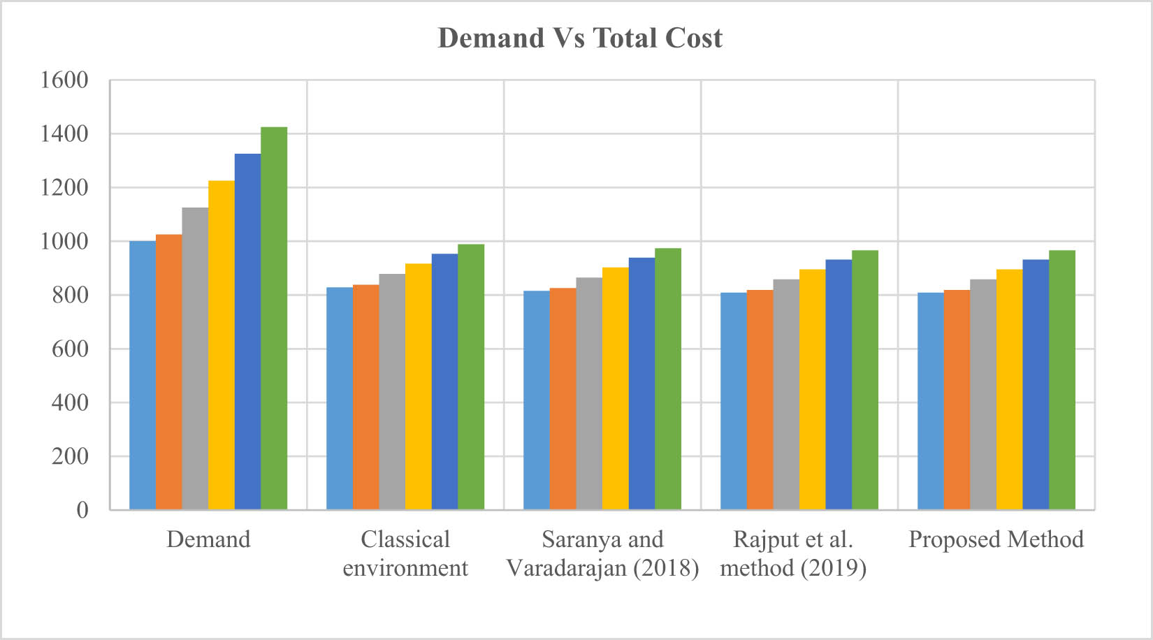
Clustered comparison with existing methods.
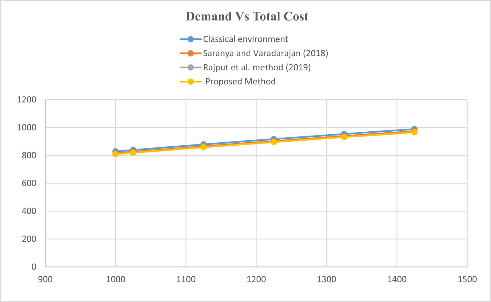
Scatter representation of existing methods.
In Example 3.1, many authors have proposed different methods to solve Rajput’s numerical problem. In the comparison study of tabular, pictorial, and logical methods, it is observed that our proposed method provides an optimal solution similar to that of Rajput et al. (2019). Our proposed method not only solves existing problems but also solves a new type of environment, which is discussed below in Example 3.2.
Example 3.2: A manufacturing facility must create an EOQ model to maximize the product's total cost. The cycle length is 6 months, with ordering costs of Rs. 20, holding costs of Rs. 04, and shortage costs of Rs. 10 per unit. We use an SVTpN membership function to capture the data’s inherent uncertainty when addressing this challenge using Neutrosophic parameters by considering the six cases discussed in Table 3.
Finding the total optimal cost under different cases
| Different cases |
|
|---|---|
| Case 1 |
|
| Case 2 |
|
| Case 3 |
|
| Case 4 |
|
| Case 5 |
|
| Case 6 |
|
Solution: After implementing equations (A5), (A6), and (A7) of our proposed method, the final total cost (TC) that we obtained is displayed in Table 4.
Tabular comparison study with some of the existing methods such as those of Sen and Malakar (2015), Saranya and Varadarajan (2018), Rajput et al. (2019)
| Demand | Sen and Malakar (2015), Saranya and Varadarajan (2018), Rajput et al. (2019) | Our proposed method |
|---|---|---|
| 1,000 | NA | 342.4935301 |
| 1,025 | NA | 632.5781217 |
| 1,125 | NA | 719.6689366 |
| 1,225 | NA | 800.3864355 |
| 1,325 | NA | 881.5672484 |
| 1,425 | NA | 981.3623184 |
We compared our proposed method with some of the existing methods such as those of Rajput et al. (2019), Saranya and Varadarajan (2018), and Sen and Malakar (2015) using both tabular and pictorial comparison studies.
In Figures 3 and 4, we can see that both figures are represented in green colour. This indicates that only our proposed method can handle this type of problem. Additionally, we observe that representations in red, blue, and light black colours do not exist in either figure. This suggests that all other existing methods are unable to handle similar uncertain situations. Hence, it is clear that our proposed method not only addresses existing numerical challenges but also tackles new types of uncertain problem types. Moreover, from the above comparison, it is clear that our proposed method is superior to some of the existing methods. Now, we are going to perform a logical comparison of Examples 3.1 and 3.2, as discussed in Table 5.
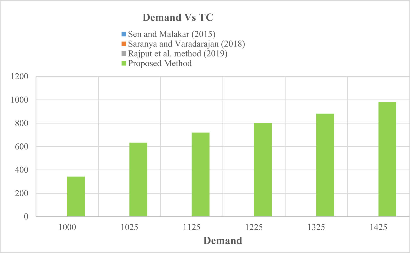
Column representation (ref Table 4).
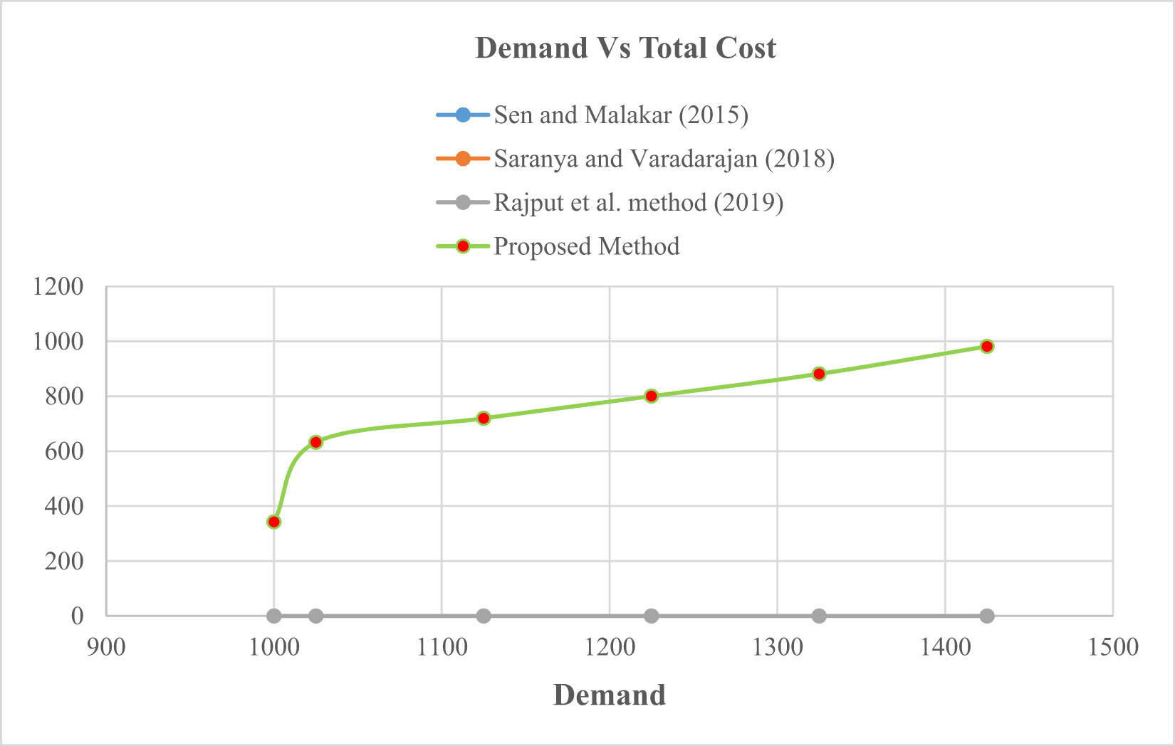
Graphical interpretation of Table 4.
Logical comparison with TC
| Examples | Comparison |
|---|---|
| Example 3.1 |
|
| Example 3.2 |
|
3.1 Logical Comparison
Table 5 lists a comparative analysis of total cost across various environmental scenarios. In Example 3.1, our observations reveal that in a fuzzy environment, the value of total cost is lower than that in a classical environment. Furthermore, in our proposed model, the total cost is observed to be lower than the classical and equal to the fuzzy environments. Additionally, in Example 3.2 it is clear that the classical and fuzzy approach is unable to provide the total cost as compared with our proposed model. That is why we said that our proposed approach not only handled the existing problem but also solved the new type of problem. To explain more about our method, we have also conducted a sensitive analysis in below Section 4.
4 Sensitive Analysis
A manufacturing facility develops an EOQ model to maximize the product's total cost. The cycle length is 6 months, and the ordering price is Rs.
Table 6 provides insights into optimizing total costs in a manufacturing setting, specifically focusing on cost-effective IM using neutrosophic theory. This sensitive analysis is crucial for decision-making in IM. Therefore, optimizing these parameters (
Sensitive analysis on proposed method
| Parameter | Change in parameters (%) |
|
|
Proposed TC |
|---|---|---|---|---|
| Proposed method | Proposed method | Proposed method | ||
|
|
13 | 47.32780723 | 14.08615158 | 357.7882502 |
| 29 | 44.83152683 | 14.87048766 | 377.7103867 | |
| 37 | 43.0753968 | 15.47673884 | 393.1091665 | |
| −13 | 48.68631097 | 13.69310292 | 347.804814 | |
| −29 | 53.37369196 | 12.4905481 | 317.2599217 | |
| −37 | 57.98788415 | 11.49665446 | 292.0150232 | |
|
|
13 | 48.65951376 | 12.12446356 | 347.9963531 |
| 29 | 47.90170815 | 10.78867301 | 353.5016597 | |
| 37 | 47.58566783 | 10.22614638 | 355.8494418 | |
| −13 | 50.43868855 | 15.19237607 | 335.7211264 | |
| −29 | 52.12240319 | 18.01465548 | 324.8762969 | |
| −37 | 53.25390911 | 19.87086161 | 317.9735275 | |
|
|
13 | 52.55684753 | 14.33368569 | 364.0756165 |
| 29 | 56.15454864 | 15.3148769 | 388.9978733 | |
| 37 | 57.86958518 | 15.78261414 | 400.8783992 | |
| −13 | 46.11579628 | 12.57703535 | 319.4566979 | |
| −29 | 41.65999947 | 11.36181804 | 288.5901781 | |
| −37 | 39.24283374 | 10.70259102 | 271.8458119 |
Based on the information from Table 6, we can conclude that the model is extremely sensitive to the holding cost, shortage cost, and total cost parameters.
The model is highly sensitive to holding cost
Similarly, if we increase the percentage in the shortage cost
Changing the
5 Conclusion
The investigation of neutrosophic set theories defines a potential use in handling inventories in our research study. Current FIMs have problems with handling uncertainty, inaccurate data, and imprecise timing, in contrast to classical models that have optimized order amounts, timing, and safety stock levels. To address these challenges, our novel approach focuses on the uncertainty associated with holding costs, shortage costs, and ordering costs, utilizing trapezoidal neutrosophic numbers. We improve decision-making procedures and offer more reliable inventory optimization solutions by utilizing neutrosophic reasoning. Notably, our method demonstrates promising results in managing inventory under uncertainty a milestone in the literature of neutrosophic sets. Additionally, Our research contributes valuable insights to enhance inventory management strategies and moderate uncertainties in EPQ operations through graphical, logical, and tabular comparisons. Despite our significant progress, several avenues for future exploration and improvement remain. These include investigating Dynamic Demand and Supply, Multi-Objective Optimization, and conducting Empirical Validation. However, it's crucial to acknowledge the limitations of our model. Its success hinges on accurate data related to costs, demand, and lead times. Obtaining precise data, especially under conditions of uncertainty, remains a challenge. Like any model, our approach is based on certain assumptions, and ongoing validation against various scenarios is essential.
Acknowledgments
The authors sincerely thank the editors and anonymous reviewers for their valuable comments and helpful feedback, which greatly improved this article.
-
Funding information: Authors state no funding involved.
-
Author contributions: All authors have accepted responsibility for the entire content of this manuscript and consented to its submission to the journal, reviewed all the results, and approved the final version of the manuscript. AD and RK designed the experiments and AD carried them out. AD developed the model code and performed the simulation. RK edited and supervised the manuscript with contributions from all co-authors.
-
Conflict of interest: Authors state no conflict of interest.
-
Data availability statement: All data supporting the reported findings in this research article are provided within the manuscript.
-
Article note: As part of the open assessment, reviews and the original submission are available as supplementary files on our website.
Appendix A Neutrosophic number and its Arithmetic and logical operators
Definition A.1
Normalized Fuzzy set (Zadeh, 1965): A fuzzy set
Definition A.2
Neutrosophic Set (Wang et al., 2010, 2011): From the universal discourse
Definition A.3
(Liang et al., 2018a,b): Let
Note: Special Case
Case 1
When
Case 2
If
Definition A.4
(Ye, 2017): Let
Definition A.5
(Ye, 2017): Let
Let
If
If
(a) If
(b) If
B EOQ Model in Neutrosophic Environment
In an environment characterized by its clarity and precision, we can determine the total cost using equation (1). However, in real-world scenarios, this cost may exhibit slight fluctuations, thereby impacting the quantity ordering (
Proposed model for finding total cost while considering the uncertainty
The neutrosophic total cost is denoted as
Now applying the def. A.4 and def. A.5, respectively, on equation (A2), we get
Initially, we have consider
Now differentiating equation (A3) with respect to
Now, similarly differentiating equation (A3) with respect to
Putting the value of
Similarly,
Therefore, optimal quantity while considering uncertainty
And, similarly, optimal shortage quantity while considering uncertainty:
This shows that
Optimal (minimum) total cost while considering uncertainty,
References
Akram, M., Alshehri, N., Davvaz, B., & Ashraf, A. (2016). Bipolar fuzzy digraphs in decision support systems. Journal of Multiple-Valued Logic & Computing, 27, 531–551.Suche in Google Scholar
Alburaikan, A., Edalatpanah, S. A., Alharbi, R., & Khalifa, H. A. (2023). Towards neutrosophic circumstances goalprogramming approach for solving multi-objective linear fractional programming problems. International Journal of Neutrosophic Science, 23(1), 350–365.10.54216/IJNS.230130Suche in Google Scholar
Alfares, H. K., & Ghaithan, A. M. (2019). EOQ and EPQ production-inventory models with variable holding cost: State-of-the-art review. Arabian Journal for Science and Engineering, 44, 1737–1755.10.1007/s13369-018-3593-4Suche in Google Scholar
Antic, S., Djordjevic Milutinovic, L., & Lisec, A. (2022). Dynamic discrete inventory control model with deterministic and stochastic demand in pharmaceutical distribution. Applied Sciences, 12(3), 1536.10.3390/app12031536Suche in Google Scholar
Butt, M. A., & Akram, M. (2016a). A new intuitionistic fuzzy rule-based decision-making system for an operating system process scheduler. Springer Plus, 5, 1–17.10.1186/s40064-016-3216-zSuche in Google Scholar
Butt, M. A., & Akram, M. (2016b). A novel fuzzy decision-making system for CPU scheduling algorithm. Neural Computing and Applications, 27, 1927–1939.10.1007/s00521-015-1987-8Suche in Google Scholar
Cárdenas-Barrón, L. E. (2011). The derivation of EOQ/EPQ inventory models with two backorders costs using analytic geometry and algebra. Applied Mathematical Modelling, 35, 2394–2407.10.1016/j.apm.2010.11.053Suche in Google Scholar
Dash, A., Giri, B. C., & Sarkar, A. K. (2023). Coordination of a single-manufacturer multi-retailer supply chain with price and green sensitive demand under stochastic lead time. Decision Making: Applications in Management and Engineering, 6(1), 679–715.10.31181/dmame0319102022dSuche in Google Scholar
Das, D., & Samanta, G. C. (2024). An EOQ model for two warehouse system during lock-down consider linear time dependent demand. Transactions on Quantitative Finance and Beyond, 1(1), 15–28.Suche in Google Scholar
Das, S. C., Zidan, A. M., Manna, A. K., Shaikh, A. A., & Bhunia, A. K. (2020). An application of preservation technology in inventory control system with price dependent demand and partial backlogging. Alexandria Engineering Journal, 59(3), 1359–1369.10.1016/j.aej.2020.03.006Suche in Google Scholar
Das, S. K. (2020). Multi item inventory model include lead time with demand dependent production cost and set-up-cost in fuzzy environment. Journal of Fuzzy Extension and Application, 1(3), 227–243.Suche in Google Scholar
Das, S. K. (2022). A fuzzy multi objective inventory model of demand dependent deterioration including lead time. Journal of Fuzzy Extension and Applications, 3(1), 1–18.Suche in Google Scholar
Duary, A., Das, S., Arif, M. G., Abualnaja, K. M., Khan, M. A. A., Zakarya, M., & Shaikh, A. A. (2022). Advance and delay in payments with the price-discount inventory model for deteriorating items under capacity constraint and partially backlogged shortages. Alexandria Engineering Journal, 61(2), 1735–1745.10.1016/j.aej.2021.06.070Suche in Google Scholar
Dubois, D., & Prade, H. (1988). Fuzzy logic in expert systems: The role of uncertainty management. Fuzzy Sets and Systems, 28, 3–17.10.1016/0165-0114(88)90030-9Suche in Google Scholar
Edalatpanah, S. A. (2023). Multidimensional solution of fuzzy linear programming. PeerJ Computer Science, 9(e1646), 1–18.10.7717/peerj-cs.1646Suche in Google Scholar
Farahbakhsh, A., & Kheirkhah, A. (2023). A new efficient genetic algorithm-Taguchi-based approach for multi-period inventory routing problem. International Journal of Research in Industrail Engineering, 12(4), 397–413.Suche in Google Scholar
Farnam, M., & Darehmiraki, M. (2021). Solution procedure for multi-objective fractional programming problem under hesitant fuzzy decision environment. Journal of Fuzzy Extension and Applications, 2(4), 364–376.Suche in Google Scholar
Gani, A. N., & Rafi, U. M. (2019). A simplistic method to work out the EOQ/EPQ with shortages by applying algebraic method and arithmetic geometric mean inequality in fuzzy atmosphere. Bulletin of Pure and Applied Sciences, 38E(1), 348–355.10.5958/2320-3226.2019.00037.7Suche in Google Scholar
Gani, A. N., & Rafi, U. M. (2020). A new method to discussing the manufacturing defects in EOQ/EPQ inventory models with shortages using fuzzy techniques. Advances and Applications in Mathematical Sciences, 19(11), 1189–1203.Suche in Google Scholar
Habib, S., Akram, M., & Ashraf, A. (2017). Fuzzy climate decision support systems for tomatoes in high tunnels. International Journal of Fuzzy Systems, 19(3), 751–775.10.1007/s40815-016-0183-zSuche in Google Scholar
Iqbal, W., Yang, T., & Ashraf, S. (2023). Optimizing earthquake response with Fermatean probabilistic hesitant fuzzy sets: A decision support framework. Journal of Operational and Strategic Analytics, 1(4), 190–197.10.56578/josa010404Suche in Google Scholar
Jani, M. Y., Patel, H. A., Bhadoriya, A., Chaudhari, U., Abbas, M., & Alqahtani, M. S. (2023). Deterioration control decision support system for the retailer during availability of trade credit and shortages. Mathematics, 11, 580.10.3390/math11030580Suche in Google Scholar
Khan, I., & Sarkar, B. (2021). Transfer of risk in supply chain management with joint pricing and inventory decision considering shortages. Mathematics, 9, 638.10.3390/math9060638Suche in Google Scholar
Liang, R. X., Wang, J. Q., & Li, L. (2018a). Multi-criteria group decision-making method based on interdependent inputs of single-valued trapezoidal neutrosophic information. Neural Computing and Applications, 30, 241–260.10.1007/s00521-016-2672-2Suche in Google Scholar
Liang, R. X., Wang, J. Q., & Zhang, H. Y. (2018b). A multi-criteria decision-making method based on single-valued trapezoidal neutrosophic preference relations with complete weight information. Neural Computing and Applications, 30, 3383–3398.10.1007/s00521-017-2925-8Suche in Google Scholar
Lin, S. S. C. (2019). Note on “The derivation of EOQ/EPQ inventory models with two backorders costs using analytic geometry and algebra”. Applied Mathematical Modelling, 73, 378–386.10.1016/j.apm.2019.04.025Suche in Google Scholar
Mashud, A. H. (2020). An EOQ deteriorating inventory model with different types of demand and fully backlogged shortages. International Journal of Logistics Systems and Management, 36, 16–45.10.1504/IJLSM.2020.107220Suche in Google Scholar
Masoomi, B., Sahebi, I. G., Arab, A., & Edalatpanah, S. A. (2023). A neutrosophic enhanced best-worst method for performance indicators assessment in the renewable energy supply chain. Soft Computing, 1–20. doi: 10.1007/s00500-023-09459-0.Suche in Google Scholar
Miriam, R., Martin, N., & Rezaei, A. (2023). Decision making on consistent customer centric inventory model with quality sustenance and smart warehouse cost parameters. Decision Making: Applications in Management and Engineering, 6(2), 341–371.10.31181/dmame622023649Suche in Google Scholar
Mohanta, K., & Sharanappa, D. (2024). Neutrosophic data envelopment analysis: A comprehensive review and current trends. Optimality, 1(1), 10–22.Suche in Google Scholar
Nazabadi, M. R., Najafi, S. E., Mohaghar, A., & Sobhani, F. M. (2024). The joint policy of production, maintenance, and product quality in multi-machine production system by reinforcement learning and agent-based modeling. International Journal of Research in Industrial Engineering, 5(1), 71–87.Suche in Google Scholar
Rajput, N., Singh, A. P., & Pandey, R. K. (2019). Optimize the cost of a fuzzy inventory model with shortage using signed distance method. International Journal of Research in Advent Technology, 7(5), 204–208.10.32622/ijrat.75201963Suche in Google Scholar
Saranya, R., & Varadarajan, R. (2018). A fuzzy inventory model with acceptable shortage using graded mean integration value method. Journal of Physics: Conference Series, 1000, 012009.10.1088/1742-6596/1000/1/012009Suche in Google Scholar
Sen, N., & Malakar, S. (2015). A fuzzy inventory model with shortages using different fuzzy numbers. American Journal of Mathematics and Statistics, 5(5), 238–248.Suche in Google Scholar
Setiawan, R. I., Lesmono, J. D., & Limansyah, T. (2021). Inventory control problems with exponential and quadratic demand considering weibull deterioration. Journal of Physics: Conference Series, 1821, 012057.10.1088/1742-6596/1821/1/012057Suche in Google Scholar
Sharma, S., Tyagi, A., Verma, B. B., & Kumar, S. (2022). An inventory control model for deteriorating items under demand dependent production with time and stock dependent demand. International Journal of Operations and Quantitative Management, 27(4), 321–336.10.46970/2021.27.4.2Suche in Google Scholar
Smarandache, F. (1999). A unifying field in logics. Neutrosophy. Neutrosophic probability, set and logic. American Research Press.Suche in Google Scholar
Sulak, H. (2015). An EOQ model with defective items and shortages in fuzzy sets environment. International Journal of Social Sciences and Education Research, 2(3), 915–929.10.24289/ijsser.279034Suche in Google Scholar
Thinakaran, N., Jayaprakas, J., & Elanchezhian, C. (2019). Survey on inventory model of EOQ & EPQ with partial backorder problems. Materials Today: Proceedings, 16, 629–635.10.1016/j.matpr.2019.05.138Suche in Google Scholar
Wang, H., Smarandache, F., Zhang, Y., & Sunderraman, R. (2010). Single valued neutrosophic sets. Infinite Study, 12, 410–413.Suche in Google Scholar
Wang, H., Zhang, Y., Sunderraman, R., & Smarandache, F. (2011). Single valued neutrosophic sets. Fuzzy Sets Rough Sets and Multivalued Operations and Applications, 3(1), 33–39.Suche in Google Scholar
Ye, J. (2017). Some weighted aggregation operators of trapezoidal neutrosophic numbers and their multiple attribute decision making method. Informatica, 28, 387–402.10.15388/Informatica.2017.108Suche in Google Scholar
Zadeh, L. (1965). Fuzzy sets. Information and Control, 8, 338–353.10.1016/S0019-9958(65)90241-XSuche in Google Scholar
© 2024 the author(s), published by De Gruyter
This work is licensed under the Creative Commons Attribution 4.0 International License.
Artikel in diesem Heft
- Regular Articles
- Political Turnover and Public Health Provision in Brazilian Municipalities
- Examining the Effects of Trade Liberalisation Using a Gravity Model Approach
- Operating Efficiency in the Capital-Intensive Semiconductor Industry: A Nonparametric Frontier Approach
- Does Health Insurance Boost Subjective Well-being? Examining the Link in China through a National Survey
- An Intelligent Approach for Predicting Stock Market Movements in Emerging Markets Using Optimized Technical Indicators and Neural Networks
- Analysis of the Effect of Digital Financial Inclusion in Promoting Inclusive Growth: Mechanism and Statistical Verification
- Effective Tax Rates and Firm Size under Turnover Tax: Evidence from a Natural Experiment on SMEs
- Re-investigating the Impact of Economic Growth, Energy Consumption, Financial Development, Institutional Quality, and Globalization on Environmental Degradation in OECD Countries
- A Compliance Return Method to Evaluate Different Approaches to Implementing Regulations: The Example of Food Hygiene Standards
- Panel Technical Efficiency of Korean Companies in the Energy Sector based on Digital Capabilities
- Time-varying Investment Dynamics in the USA
- Preferences, Institutions, and Policy Makers: The Case of the New Institutionalization of Science, Technology, and Innovation Governance in Colombia
- The Impact of Geographic Factors on Credit Risk: A Study of Chinese Commercial Banks
- The Heterogeneous Effect and Transmission Paths of Air Pollution on Housing Prices: Evidence from 30 Large- and Medium-Sized Cities in China
- Analysis of Demographic Variables Affecting Digital Citizenship in Turkey
- Green Finance, Environmental Regulations, and Green Technologies in China: Implications for Achieving Green Economic Recovery
- Coupled and Coordinated Development of Economic Growth and Green Sustainability in a Manufacturing Enterprise under the Context of Dual Carbon Goals: Carbon Peaking and Carbon Neutrality
- Revealing the New Nexus in Urban Unemployment Dynamics: The Relationship between Institutional Variables and Long-Term Unemployment in Colombia
- The Roles of the Terms of Trade and the Real Exchange Rate in the Current Account Balance
- Cleaner Production: Analysis of the Role and Path of Green Finance in Controlling Agricultural Nonpoint Source Pollution
- The Research on the Impact of Regional Trade Network Relationships on Value Chain Resilience in China’s Service Industry
- Social Support and Suicidal Ideation among Children of Cross-Border Married Couples
- Asymmetrical Monetary Relations and Involuntary Unemployment in a General Equilibrium Model
- Job Crafting among Airport Security: The Role of Organizational Support, Work Engagement and Social Courage
- Does the Adjustment of Industrial Structure Restrain the Income Gap between Urban and Rural Areas
- Optimizing Emergency Logistics Centre Locations: A Multi-Objective Robust Model
- Geopolitical Risks and Stock Market Volatility in the SAARC Region
- Trade Globalization, Overseas Investment, and Tax Revenue Growth in Sub-Saharan Africa
- Can Government Expenditure Improve the Efficiency of Institutional Elderly-Care Service? – Take Wuhan as an Example
- Media Tone and Earnings Management before the Earnings Announcement: Evidence from China
- Review Articles
- Economic Growth in the Age of Ubiquitous Threats: How Global Risks are Reshaping Growth Theory
- Efficiency Measurement in Healthcare: The Foundations, Variables, and Models – A Narrative Literature Review
- Rethinking the Theoretical Foundation of Economics I: The Multilevel Paradigm
- Financial Literacy as Part of Empowerment Education for Later Life: A Spectrum of Perspectives, Challenges and Implications for Individuals, Educators and Policymakers in the Modern Digital Economy
- Special Issue: Economic Implications of Management and Entrepreneurship - Part II
- Ethnic Entrepreneurship: A Qualitative Study on Entrepreneurial Tendency of Meskhetian Turks Living in the USA in the Context of the Interactive Model
- Bridging Brand Parity with Insights Regarding Consumer Behavior
- The Effect of Green Human Resources Management Practices on Corporate Sustainability from the Perspective of Employees
- Special Issue: Shapes of Performance Evaluation in Economics and Management Decision - Part II
- High-Quality Development of Sports Competition Performance Industry in Chengdu-Chongqing Region Based on Performance Evaluation Theory
- Analysis of Multi-Factor Dynamic Coupling and Government Intervention Level for Urbanization in China: Evidence from the Yangtze River Economic Belt
- The Impact of Environmental Regulation on Technological Innovation of Enterprises: Based on Empirical Evidences of the Implementation of Pollution Charges in China
- Environmental Social Responsibility, Local Environmental Protection Strategy, and Corporate Financial Performance – Empirical Evidence from Heavy Pollution Industry
- The Relationship Between Stock Performance and Money Supply Based on VAR Model in the Context of E-commerce
- A Novel Approach for the Assessment of Logistics Performance Index of EU Countries
- The Decision Behaviour Evaluation of Interrelationships among Personality, Transformational Leadership, Leadership Self-Efficacy, and Commitment for E-Commerce Administrative Managers
- Role of Cultural Factors on Entrepreneurship Across the Diverse Economic Stages: Insights from GEM and GLOBE Data
- Performance Evaluation of Economic Relocation Effect for Environmental Non-Governmental Organizations: Evidence from China
- Functional Analysis of English Carriers and Related Resources of Cultural Communication in Internet Media
- The Influences of Multi-Level Environmental Regulations on Firm Performance in China
- Exploring the Ethnic Cultural Integration Path of Immigrant Communities Based on Ethnic Inter-Embedding
- Analysis of a New Model of Economic Growth in Renewable Energy for Green Computing
- An Empirical Examination of Aging’s Ramifications on Large-scale Agriculture: China’s Perspective
- The Impact of Firm Digital Transformation on Environmental, Social, and Governance Performance: Evidence from China
- Accounting Comparability and Labor Productivity: Evidence from China’s A-Share Listed Firms
- An Empirical Study on the Impact of Tariff Reduction on China’s Textile Industry under the Background of RCEP
- Top Executives’ Overseas Background on Corporate Green Innovation Output: The Mediating Role of Risk Preference
- Neutrosophic Inventory Management: A Cost-Effective Approach
- Mechanism Analysis and Response of Digital Financial Inclusion to Labor Economy based on ANN and Contribution Analysis
- Asset Pricing and Portfolio Investment Management Using Machine Learning: Research Trend Analysis Using Scientometrics
- User-centric Smart City Services for People with Disabilities and the Elderly: A UN SDG Framework Approach
- Research on the Problems and Institutional Optimization Strategies of Rural Collective Economic Organization Governance
- The Impact of the Global Minimum Tax Reform on China and Its Countermeasures
- Sustainable Development of Low-Carbon Supply Chain Economy based on the Internet of Things and Environmental Responsibility
- Measurement of Higher Education Competitiveness Level and Regional Disparities in China from the Perspective of Sustainable Development
- Payment Clearing and Regional Economy Development Based on Panel Data of Sichuan Province
- Coordinated Regional Economic Development: A Study of the Relationship Between Regional Policies and Business Performance
- A Novel Perspective on Prioritizing Investment Projects under Future Uncertainty: Integrating Robustness Analysis with the Net Present Value Model
- Research on Measurement of Manufacturing Industry Chain Resilience Based on Index Contribution Model Driven by Digital Economy
- Special Issue: AEEFI 2023
- Portfolio Allocation, Risk Aversion, and Digital Literacy Among the European Elderly
- Exploring the Heterogeneous Impact of Trade Agreements on Trade: Depth Matters
- Import, Productivity, and Export Performances
- Government Expenditure, Education, and Productivity in the European Union: Effects on Economic Growth
- Replication Study
- Carbon Taxes and CO2 Emissions: A Replication of Andersson (American Economic Journal: Economic Policy, 2019)