Simulation on impact response of FMLs: effect of fiber stacking sequence, thickness, and incident angle
-
Bin Yang
 ,
Liang He
,
Liang He

Abstract
We built a three-dimensional finite element (FE) model to investigate the impact response of fiber-metal laminates (FMLs). This FE model comprises two metal layers as facesheets and a carbon woven fabric-reinforced plastic laminate as inner core. Simulation was performed on ABAQUS/Explicit platform, and stiffness progressive degeneration criteria were implemented to evaluate damages in composites. The Johnson-Cook model was selected to calculate failures in metal, while surface-based cohesive behavior was adopted to simulate the delamination phenomenon. We studied the fiber stacking sequence, panel thickness, and incident angle effect on the impact behavior of FMLs. The critical penetration energy of the FMLs was determined, and the impact parameter history was discussed.
1 Introduction
Lightweight composite materials are currently finding extensive applications in load-bearing engineering areas. Fiber-metal laminates (FMLs) usually consist of two thin metal layers and continuous fiber-reinforced plastic (FRP) composite laminates. FMLs are novel hybrid composites with high fatigue and impact resistance ability. In real engineering fields, high-velocity impact performance is one of the important safety issues. Even though FMLs could enhance the energy absorption and increase the critical penetration velocity when compared with any of their components [1, 2], the damage mechanism of FMLs after experiencing the impact event need to be investigated more.
According to the velocity, the impact event can be divided into low-velocity (≤11 m/s), high-velocity (≥11 m/s), ballistic (≥500 m/s), and hypervelocity impact (≥2000 m/s). All these impact events can result in internal damages in FMLs, which could further cause severe strength and stability reduction of the structure. For the FRP plate in an impact event, internal damage is formed extending beyond the contact area [3]. However, FMLs did not show such an undesirable response [4]. Experiments and simulation researches have investigated the response of FMLs under high-velocity impact tests [5, 6]. Compared with experimental methods, the finite element (FE) approaches appear to be the best technique for analyzing the behavior of composite laminates [7, 8]. Simulation techniques on FMLs under high-velocity impact load rely on four approaches: damage mechanics, fracture mechanics, failure criteria, and plasticity [9]. Development of a reliable FE model to predict FMLs under high-velocity impact load requires the implementation of suitable failure criteria. For damages in composite materials, material and geometric non-linearity are the limiting factors of analytical models [10]. Many criteria are available to detect the failure status of composite laminates, such as maximum stress, Tsai-Wu, and Chang-Chang failure criteria. Among these, the Hashin criteria are the most classical criteria. To describe the elastic-plastic response of the metals, an isotropic constitutive model based on the Johnson-Cook material model is always used [11, 12]. Also, modeling of impacts on FMLs requires understanding the interaction status between composite and metal layers. Even though many methods have been developed for delamination prediction [13, 14], cohesive-based methods have been frequently applied to study delamination growth [8].
We developed a model to simulate FML behaviors in high-velocity (V0≤500 m/s) and ballistic (500 m/s<V0≤900 m/s) impact tests. The FE work was performed by using ABAQUS/Explicit with the assistance of a user-defined subroutine program. We tested the impact performance of the model with initial velocity up to 900 m/s. The effects of fiber stacking sequence, composite layer thickness, and incident direction on the impact performance of the built FE model were investigated.
2 Simulation method
A three-dimensional (3D) FE model based on the progressive damage theory is developed to simulate failures in FMLs [15]. The flowchart of the subroutine is shown in Figure 1. This 3D model is based on the Hashin failure criteria that include six different failure modes. In detail, the modes consisted of warp and fill fiber tensile failure, compression failure, and matrix tensile and compression failure of the FRP composites, as listed in Table 1. In impact simulation, element failure occurs when any of the failure criteria is satisfied (e≥1); then, the element stiffness will reduce to a special percentage of its original value according to Table 2. When eftw≥1 and eftf≥1 appear together, the element will be deleted and cannot further carry load. All the parameters used in the FE model are inputted according to the experimental results in Ref. [16], as listed in Table 3. In terms of the interface between metal and its neighbor composites, surface-based cohesive behavior (SBCB) was employed to simulate the delamination [17]. The traction-separation damage law of SBCB is shown in Figure 2. The maximum separation criterion was employed as the damage initiation criteria, which can be represented as

Degradation criteria flowchart of VUMAT in the FE method.
Damage modes for FRPs in the impact simulation in VUMAT program.
| Damage mode | Criteria |
|---|---|
| Fiber tensile damage in warp direction | |
| Fiber compression damage in warp direction | |
| Fiber tensile damage in fill direction | |
| Fiber compression damage in fill direction | |
| Matrix compression damage | |
| Matrix tensile damage |
Material stiffness degradation rule for composite layer in FMLs.
| Failure mode | WGF/epoxy and WCF/epoxy composites |
|---|---|
| Warp fiber tensile breaking (eftw≥1) | E11=0.1E11, G12=0.1G12, G13=0.1G13, v12=0.1v12, v13=0.1v13 |
| Warp fiber compress buckling (efcw≥1) | E11=0.2E11, G12=0.2G12, G13=0.2G13, v12=0.2v12, v13=0.2v13 |
| Fill fiber tensile breaking (eftf≥1) | E22=0.1E22, G12=0.1G12, G23=0.1G23, v12=0.1v12, v23=0.1v23 |
| Fill fiber compress buckling (efcf≥1) | E22=0.2E22, G12=0.2G12, G23=0.2G23, v12=0.2v12, v23=0.2v23 |
| Z direction tensile breaking (edt≥1) | E33=0.1E33, G13=0.1G13, G23=0.1G23, v13=0.1v12, v23=0.1v23 |
| Z direction compress buckling (edc≥1) | E33=0.2E33, G13=0.2G13, G23=0.2G23, v13=0.2v12, v23=0.2v23 |
Strength properties of composites (MPa) and elastic properties of composites (GPa) in the simulation.
| Materials | XT=YT | S12=S13=S23 | XC=YC | ZT | ZC | E11=E22 | E33 | G12 | G13=G23 | v12 | v13=v23 | ρ (kg/m3) |
|---|---|---|---|---|---|---|---|---|---|---|---|---|
| WGFRP | 500 | 66 | 370 | 49.5 | 22 | 50.3 | 8.1 | 3.79 | 3.7 | 0.058 | 0.037 | 1460 |

Traction-separation theory.
Kn, Ks and Kt are normal and tangential stiffness components; tnmax, tsmax, and ttmax: peak values of the contact stress; δnmax, δsmax, and δtmax: peak values of the contact separation; δnf, δsf, and δtf: separations at failure. (A) Traction-separation behavior. (B) Damage modeling for cohesive surfaces.
In terms of interface damage evolution, a scalar damage variable, D, was used to represent the overall damage at the contact point. The contact stress components are affected by the damage according to
where
The Johnson-Cook model [18] was selected to characterize the metal property degradation due to perforation. The model can be characterized by the yield stress as follows:
where A, B, C,
reaches 1. In this expression, the equivalent strain to fracture δf is defined as follows:
where d1 to d5 are material constants, which can be determined from experiments; p is the hydrostatic pressure;
Model parameters and material models for the Johnson-Cook damage model.
| Density (kg/m3) | Young’s modulus (GPa) | Poisson’s ratio | A | B | n | m | d1 | d4 |
|---|---|---|---|---|---|---|---|---|
| 8000 | 207.8 | 0.3 | 280 | 803 | 0 | 1 | 0.69 | 0.05 |
2 Simulation results and discussion
The FE model with dimension of 50×50 mm2 is shown in Figure 3. All meshes are of type C3D8R, and the element is an eight-node hexahedral solid brick element. A refinement mesh region was adopted in the potential contact area of the model to catch the results with higher accuracy. To investigate the model configuration effect on the impact response of FMLs, we studied a model with different ply orientation, layer thickness, and impact direction. In detail, the FML layer mode comprises [M/90n/M] and [M/45n/M], and the composites layer thickness varies from one to eight layers (with thickness of 0.5 mm for each layer), while the projectile direction changes from 10° to 90°.

FE model used in the ballistic impact simulation.
3.1 Ply mode effect on the impact performance of FMLs
3.1.1 High-velocity impact response
Figure 4 depicts the velocity and deflection curves of [M/908/M] and [M/458/M] as a function of contact time (V-t and d-t) with projectile speed from 100 to 400 m/s. With increasing of t, the projectile velocity declines from the initial velocity (V0) to 0 m/s. Then, the curves show negative velocities, which implies the rebounding of projectile. The residual velocity (Vr) of the projectile appears as a negative section in the figure. From d-t curves, deflection of both specimens subjected to V0<300 m/s recovers to the initial position after reaching the maximum deformation with increasing of contact time. However, when V0 increases to 300 and 400 m/s, the deformation could not completely recover to its initial position and permanent deformation occurs. This is mainly due to the existence of metal layers in the FMLs. Because plastic deformation in metal happens under higher impact energy (V0=300 m/s, 400 m/s), the stiffer metal layer hinders the deflection recovery of composites layers, and this further causes a permanent deformation. By comparison, we can conclude that the stacking sequence has very little influence when V0<400 m/s. Figure 5 describes the comparison result of maximum displacement (Md) and its corresponding contact time. As seen, Md and its contact time show an increasing tendency with increasing of V0. For [M/908/M], Md is 0.72 mm at 0.035 ms and V0=100 m/s. It increases to 8.88 mm at 0.044 ms when V0 increases to 500 m/s. Generally, there is no significant difference between the two FMLs when V0<500 m/s. However, both contact time and Md of [M/±458/M] increase significantly at V0=500 m/s. This is mainly due to the super in-plane shear stress capacity. At V0=500 m/s, the contact metal surface is perforated and the inner composites layers could bear some impact load.
![Figure 4: Comparison of velocity-time and deflection-time curves of different FML specimens in high-velocity impact tests (V0<500 m/s). (A) V-t curve of [M/908/M]. (B) V-t curve of [M/±458/M]. (C) d-t curve of [M/908/M]. (D) d-t curve of [M/±458/M].](/document/doi/10.1515/secm-2016-0226/asset/graphic/j_secm-2016-0226_fig_004.jpg)
Comparison of velocity-time and deflection-time curves of different FML specimens in high-velocity impact tests (V0<500 m/s). (A) V-t curve of [M/908/M]. (B) V-t curve of [M/±458/M]. (C) d-t curve of [M/908/M]. (D) d-t curve of [M/±458/M].

Comparison of maximum displacement (Md) and its corresponding contact time of different FMLs in impact tests.
One of the important considerations in designing FMLs is their perforation threshold velocity (PTV). Figure 6 shows the PTV-t curve of the two specimens. As seen, the curves decline from the initial velocity to 0 m/s. The impact energy of the projectile is fully absorbed by the specimens through various damage modes. However, the PTV of [M/458/M] is 530 m/s, while that of [M/908/M] is 540 m/s. Figure 7 shows the variation of projectile velocity versus deflection (V-d) under various V0. Below PTV, the velocity decreases in a parabolic shape and reaches zero at the maximum displacement. Afterwards, the velocity shows negative values and its absolute value increases with decreasing of displacement. Then, the velocity reaches a constant value, which implies the rebounding of projectile. For V0=PTV, the velocity declines directly to 0 after reaching the maximum value, which represents that the specimens are undergoing complete perforation. The Vr/V0 ratio could be used to further describe the behavior of the material under impact load. The Vr/V0 ratio calculated from Figure 7A and B is shown in Figure 7C. Clearly in the figure, the Vr/V0 ratio changes from the negative value to zero with increasing of V0.

Penetration threshold velocity of two FMLs with different fiber stacking sequences.
![Figure 7: Variation of impact velocity of different FMLs as a function of deflection in high velocity impact test.In the bar, N denotes negative, while P denotes positive value. (A) V-d curve of [M/908/M]. (b) V-d curve of [M/±458/M]. (c) Ratio of residual velocity to initial velocity.](/document/doi/10.1515/secm-2016-0226/asset/graphic/j_secm-2016-0226_fig_007.jpg)
Variation of impact velocity of different FMLs as a function of deflection in high velocity impact test.
In the bar, N denotes negative, while P denotes positive value. (A) V-d curve of [M/908/M]. (b) V-d curve of [M/±458/M]. (c) Ratio of residual velocity to initial velocity.
3.1.2 Ballistic impact response
Figure 8 shows the velocity history (V-t), V-d, and Vr/V0 ratio as the function of V0 in the ballistic impact test (V0<900 m/s). As seen, all the FMLs are penetrated, and the velocity decreases to a special value after impact. Unlike the V-d curve in rebounding case, the velocity of the panel decreases directly to its minimum value with increasing of deflection. The difference of the Vr/V0 ratio between [M/458/M] and [M/908/M] at V0=550 and 600 m/s is larger, and it becomes smaller when V0 is increased. Figure 9 shows the residual and absorbed impact kinetic energy calculated by Newton’s law. The fitting results between absorbed energy (EA) and initial energy (E0) of [M/458/M] and [M/908/M] are listed in Tables 5 and 6. By comparison, all the incident energy is absorbed by [M/458/M] and [M/908/M] once the incident energy is smaller than the critical penetration energy. However, if the incident energy is beyond the penetration energy, the stacking sequence with the structural style of [M/458/M] absorbs more energy. The delamination area on both sides of the FML laminates after V0=900 m/s impact test is shown in Figure 10. As seen, the delamination area on both the upper and bottom surfaces of [M/±458/M] is larger than that of [M/908/M]. Mainly due to the mismatch of deformation between metal and ±45° fiber layers, the opportunity of delamination between them is improved.
![Figure 8: Projectile impactor velocity as the function of contact time and displacement and Vr/V0 ratio of the two specimens in the ballistic impact simulation.(A) V-t curve of [M/908/M]. (B) V-t curve of [M/±458/M]. (C) V-d curve of [M/908/M]. (D) V-d curve of [M/±458/M]. (E) Ratio of residual velocity to initial velocity.](/document/doi/10.1515/secm-2016-0226/asset/graphic/j_secm-2016-0226_fig_008.jpg)
Projectile impactor velocity as the function of contact time and displacement and Vr/V0 ratio of the two specimens in the ballistic impact simulation.
(A) V-t curve of [M/908/M]. (B) V-t curve of [M/±458/M]. (C) V-d curve of [M/908/M]. (D) V-d curve of [M/±458/M]. (E) Ratio of residual velocity to initial velocity.
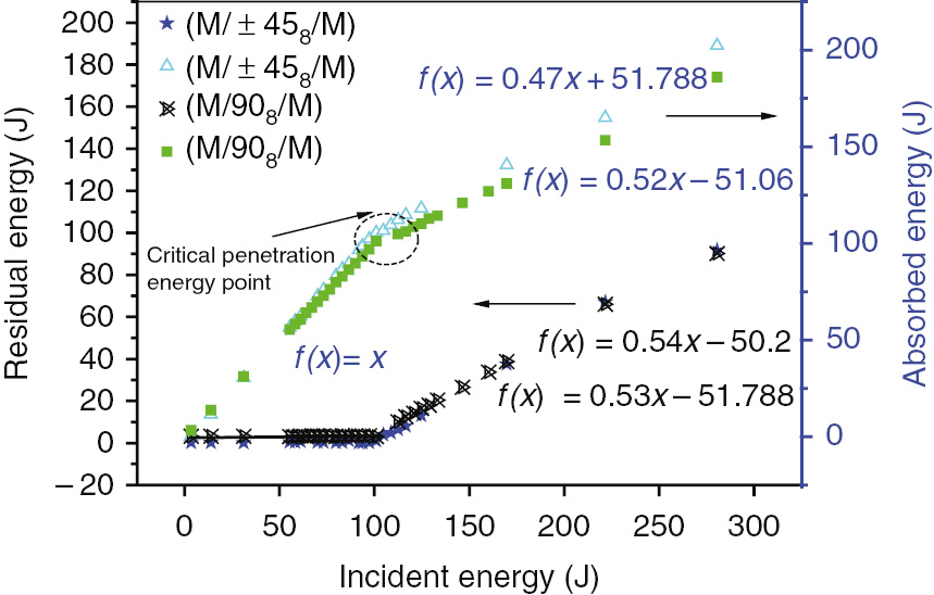
Incident energy vs. residual impact energy in high-velocity impact simulation.
Fitting results of [M/±458/M] specimens.
| Equation | y=a+bx | Standard error |
|---|---|---|
| Adj. R-square | 0.99529 | – |
| Intercept | 51.788 | 2.69 |
| Slope | 0.47 | 0.015 |
Fitting results of [M/908/M] specimens.
| Equation | y=a+bx | Standard error |
|---|---|---|
| Adj. R-square | 0.99658 | – |
| Intercept | −51.06 | 2.15 |
| Slope | 0.52 | 0.012 |

Comparison between delamination areas between fiber and metal in the two specimens (V0=900 m/s).
3.1.3 Damage patterns of FMLs in impact simulation
The damage patterns of [M/908/M] are shown in Figure 11. From the failure morphology of the panel under various impact situations, the impact event finished in 0.08 ms when V0≤540 m/s, while it takes merely 0.04 ms when V0≥700 m/s. The initial impact energy exceeds the penetration threshold of the FML panel at V0=540 m/s. Below this velocity, the impact energy is consumed by contact metal face deformation (V0=100 m/s) or the dent formed in the material (V0=400 m/s). When the panel is completely penetrated, severe stress in the bottom metal is found. Mainly because of the brittle nature of fibers, fiber breaking in the FMLs after being penetrated is the major damage mode. With increasing of contact duration between FMLs and projectile, cracks in metal are generated and then propagate to the inner composite layers.
![Figure 11: Cross-section stress history in [M/908/M] in the impact event at various velocities.](/document/doi/10.1515/secm-2016-0226/asset/graphic/j_secm-2016-0226_fig_011.jpg)
Cross-section stress history in [M/908/M] in the impact event at various velocities.
3.2 FML thickness effect
In Figure 12, the velocity history of [M/±45n/M] and [M/90n/M] at V0=540 m/s is compared. Here, we use subscript n to indicate the composite layer numbers in the FMLs. At the same V0, velocity decreases with increasing of t. The contact time also decreases with decreasing of FML thickness. Except the [M/908/M] specimen, all the panels are penetrated and they leave a positive Vr after impact. Vr shows an increasing tendency with decreasing of FML thickness, which indicates the decline of absorbed energy. A comparison between absorbed energy-thickness curves is given in Figure 13A. As seen, when the incident impact energy is beyond the critical penetration energy, the incident energy absorbed by [M/±45n/M] is higher than [M/90n/M]. The situation is opposite while incident energy is equal or near the penetration value. Figure 13 also shows the Vr/V0 tendency as the function of thickness. Generally, the Vr/V0 value changes similarly with energy. With increasing of thickness, Vr/V0 decreases. However, data for [M/90n/M] decline to 0 at eight layers, while the other specimens have positive values, which indicate that the panel was completely penetrated. Figure 14 compares the damage pattern of the two FMLs with different thicknesses at V0=540 m/s. As seen, all the specimens with composite thickness less than eight layers are completely penetrated.

Velocity history as the function of specimen thickness (V0=540 m/s).

Absorbed energy and Vr/V0 as the function of FML thickness.
(A) Absorbed energy-thickness. (B) Vr/V0-thickness.

Damage patterns of FMLs under impact velocity of 540 m/s.
3.3 Effect of projectile incident angle on the impact properties of FMLs
Figure 15 is the schematic diagram of the incident angle definition. Figure 16 depicts the V-t and d-t curves of [M/908/M] at V0=600 m/s and θ=10–90°. As seen, no negative velocities are shown. With increasing of θ, the residual velocity (Vr) firstly decreases and then increases. The Vr/V0 ratio as a function of θ is shown in Figure 17A. All the Vr/V0 is positive, and it decreases from 0.75 (θ=10°) to the minimum value at θ=50°. Then, the curve shows an increasing tendency. This phenomenon can be explained as follows: with small θ, the projectile is rebounded, attributed to the smaller velocity component in normal direction. With increasing of θ, the panel is penetrated, and the increased traveled path consumes the projectile energy. As a result, the residual velocity is becoming smaller. However, the panel is completely penetrated when θ>60°, and the energy is absorbed by various damage modes in FMLs. From the d-t curves at various θ, the displacement of projectile shows the same tendency at t=0.1 ms. The deformation increases with increasing of contact time for θ=10° and 20°, while it keeps the same level after reaching the maximum for θ=30°–60°. A comparison of projectile displacement when t=0.1 ms is shown in Figure 17B. As seen, the displacement for θ=30°–60° is the smallest among all the specimens. The damage pattern of the contact surface of FMLs after impact is shown in Figure 18. As seen, when θ=10° and 20°, the three panels are not penetrated, and the projectile leaves a large broken area. For θ=30°–60°, the panels are penetrated and an oblique hole on the specimens is found. This is especially obvious for θ=50°. For θ=70°, 80°, and 90°, the panel is completely penetrated mainly due to the larger incident energy. The hole shape is circular for θ=90°; however, it is elliptical instead in oblique impact.

Schematic diagram of the incident angle in ballistic impact simulation.

Contact time-based curves of the FMLs as the function of incident angle (V0=600 m/s for all cases).
(A) V-t curve. (B) d-t curve.

Vr/V0 ratio and displacement when contact time equal to 0.1 ms is the function of incident angle.
(A) Vr/V0-θ. (B) Projectile displacement-θ.
![Figure 18: Damage pattern of [M/908/M] FMLs in V0=600 m/s impact test with various incident angles.](/document/doi/10.1515/secm-2016-0226/asset/graphic/j_secm-2016-0226_fig_018.jpg)
Damage pattern of [M/908/M] FMLs in V0=600 m/s impact test with various incident angles.
4 Conclusion
We built a 3D FE FML model to simulate the impact test. We implemented a user-material subroutine to evaluate composite damage, the Johnson-Cook material model to calculate metal broken failure, and the SBCB method to simulate delamination. The following conclusions can be drawn:
Under critical penetration velocity, the fiber stacking sequence in FMLs has very limited influence on the impact performance; while above this velocity, [M/458/M] could absorb more incident energy than [M/908/M] due to the larger delamination area.
The critical penetration energy of [M/908/M] is larger than that of [M/±458/M]. With increasing of thickness, the absorbed energy increases. [M/±45n/M] absorbs more energy than [M/90n/M] when the composite layers are less than seven.
The projectile incident angle affects the damage pattern. The projectile is rebounded when θ<30°, and the panel is penetrated for other cases. The residual velocity of the projectile is the least among all the researched conditions when θ=50°.
Acknowledgment
This work is financially supported by the National Natural Science Foundation of China (no. 51605164).
References
[1] Alderliesten RC, Homan JJ. Int. J. Fatigue 2006, 28, 1116–1123.10.1016/j.ijfatigue.2006.02.015Suche in Google Scholar
[2] Sitnikova E, Guan ZW, Schleyer GK. Int. J. Solids Struct. 2014, 51, 3135–3146.10.1016/j.ijsolstr.2014.05.010Suche in Google Scholar
[3] Yang B, Wang ZQ, Zhou LM, Zhang JF, Liang WY. Compos. Struct. 2015, 132, 464–476.10.1016/j.compstruct.2015.05.069Suche in Google Scholar
[4] Yaghoubi AS, Liaw B. Int. J. Impact Eng. 2013, 54, 138–148.10.1016/j.ijimpeng.2012.10.007Suche in Google Scholar
[5] Edison EH, Jerzy AS, Akindele GO. Compos. Part A 2016, 87, 54–65.10.1016/j.compositesa.2016.04.007Suche in Google Scholar
[6] Zohreh A, Taheri F. Compos. Struct. 2016, 140, 136–146.10.1016/j.compstruct.2015.12.015Suche in Google Scholar
[7] Yu GC, Wu LZ, Ma L, Xiong J. Compos. Struct. 2015, 119, 757–766.10.1016/j.compstruct.2014.09.054Suche in Google Scholar
[8] Chai GB, Manikandan P. Compos. Struct. 2014, 107, 363–381.10.1016/j.compstruct.2013.08.003Suche in Google Scholar
[9] Iannucci L. Int. J. Impact Eng. 2006, 32, 1013–1043.10.1016/j.ijimpeng.2004.08.006Suche in Google Scholar
[10] Moriniere FD, Alderliesten RC, Benedictus R. Int. J. Impact Eng. 2014, 67, 27–38.10.1016/j.ijimpeng.2014.01.004Suche in Google Scholar
[11] Johnson GR, Cook WH. In Seventh International Symposium on Ballistics, The Hague, Netherlands, 1983, 541–547.Suche in Google Scholar
[12] Buyuk M, Kan S, Loikkanen MJ. J. Aerosp. Eng. 2009, 22, 287–295.10.1061/(ASCE)0893-1321(2009)22:3(287)Suche in Google Scholar
[13] Krueger R, Minguet PJ, Brien TK. ASTM STP 1383; NASA Langley Research Center 2000, 105–128.Suche in Google Scholar
[14] Balzani C, Wagner W. Eng. Fract. Mech. 2008, 75, 2597–2615.10.1016/j.engfracmech.2007.03.013Suche in Google Scholar
[15] Hashin Z. J. Appl. Mech. 1980, 47, 329–334.10.1115/1.3153664Suche in Google Scholar
[16] Naik NK, Sekher YC, Meduri S. J. Reinf. Plast. Comp. 2000, 19, 912–954.10.1106/X80M-4UEF-CPPK-M15ESuche in Google Scholar
[17] Abaqus 6.9 Example Problems Manual 1.4.6. Dassault Systèmes Simulia Corporation, 2010.Suche in Google Scholar
[18] Johnson G, Cook W. Eng. Fract. Mech. 1985, 21, 31–48.10.1016/0013-7944(85)90052-9Suche in Google Scholar
©2017 Walter de Gruyter GmbH, Berlin/Boston
This article is distributed under the terms of the Creative Commons Attribution Non-Commercial License, which permits unrestricted non-commercial use, distribution, and reproduction in any medium, provided the original work is properly cited.
Artikel in diesem Heft
- Frontmatter
- Original articles
- Review of the mechanical performance of variable stiffness design fiber-reinforced composites
- Exact solution for bending analysis of functionally graded micro-plates based on strain gradient theory
- Synthesis, microstructure, and mechanical properties of in situ TiB2/Al-4.5Cu composites
- Microstructure and properties of W-Cu/1Cr18Ni9 steel brazed joint with different Ni-based filler metals
- Drilling studies on the prepared aluminum metal matrix composite from wet grinder stone dust particles
- Studies on mechanical properties of thermoplastic composites prepared from flax-polypropylene needle punched nonwovens
- Design of and with thin-ply non-crimp fabric as building blocks for composites
- Effect of coir fiber reinforcement on mechanical properties of vulcanized natural rubber composites
- Investigation and analysis of glass fabric/PVC composite laminates processing parameters
- Abrasive wear behavior of silane treated nanoalumina filled dental composite under food slurry and distilled water condition
- Finite element study into the effects of fiber orientations and stacking sequence on drilling induced delamination in CFRP/Al stack
- Preparation of PAA/WO3 composite films with enhanced electrochromism via layer-by-layer method
- Effect of alkali treatment on hair fiber as reinforcement of HDPE composites: mechanical properties and water absorption behavior
- Integration of nano-Al with one-step synthesis of MoO3 nanobelts to realize high exothermic nanothermite
- A time-of-flight revising approach to improve the image quality of Lamb wave tomography for the detection of defects in composite panels
- The simulation of the warpage rule of the thin-walled part of polypropylene composite based on the coupling effect of mold deformation and injection molding process
- Novel preparation method and the characterization of polyurethane-acrylate/ nano-SiO2 emulsions
- Microwave properties of natural rubber based composites containing carbon black-magnetite hybrid fillers
- Simulation on impact response of FMLs: effect of fiber stacking sequence, thickness, and incident angle