Spatial effects with missing data
-
Matías Guzmán Naranjo
 ,
Miri Mertner
,
Miri Mertner

Abstract
In recent years, there has been an increased attention and interest in quantitative and statistical models of language contact and language diffusion in space. This article presents an improved model, multivAreate 2, to estimate spatial and contact relations between languages and dialects based on work by Guzmán Naranjo and Mertner ((2022). Estimating areal effects in typology: A case study of african phoneme inventories. Journal of Linguistic Typology 27(2), 455–80) and Ranacher et al. ((2021). Contact-tracing in cultural evolution: A Bayesian mixture model to detect geographic areas of language contact. Journal of the Royal Society Interface 18(181), 1–15). We test our model on three different datasets: Balkans, South America (Ranacher et al. (2021). Contact-tracing in cultural evolution: A Bayesian mixture model to detect geographic areas of language contact. Journal of the Royal Society Interface 18(181), 1–15), and the Americas (Urban et al., (2019). The areal typology of western middle and south america: Towards a comprehensive view. Linguistics 57(6), 1403–63). We show that this new model can address shortcomings found in previous models, and it offers some useful tools for researchers working on contact and areal linguistics.
1 Introduction
The description of geographical patterns in linguistic structure and their causes is among the primary aims for dialectologists, sociolinguists, and areal typologists (e.g. Balthasar and Nichols 2006, Bisang 2006, Muysken 2008, Aikhenvald 2006, Güldemann 2018, Bickel 2007, Trudgill 1974). In theory, the classical notion of the linguistic area or Sprachbund in contact linguistics can be defined as a region in which languages converge towards a particular typological profile that is not explained by the genealogical relationships between them or by typological universals (see e.g. Joseph 2020, Bisang 2006, Matras 2011, for a more in-depth discussion of definitions and related issues). The linguistic area is the net result of numerous local interactions between a network of speakers of the languages involved, at least some of whom are bilingual or multilingual (Joseph 1999).
As discussed at length in the literature too vast to summarise here, the notion of linguistic area is riddled with problems. To begin with, first, it is often not trivial to decide unambiguously which languages do and do not take part in a linguistic area. As Haspelmath (2001, 1504) states, “Membership in a Sprachbund is often a matter of degree” (see also Campbell 2017, for a discussion on non-discrete linguistic areas). One of the consequences of this is that the boundaries of a linguistic area may be somewhat diffuse, with some languages considered ‘core members’ and others ‘peripheral’ or ‘partial members’. Moreover, linguistic areas can overlap; their boundaries are not so discrete so that languages can belong to more than one linguistic area. This follows from the emergent character of linguistic areas as the result of multifarious contact events through time. Different groups of speakers of a language may interact with speakers from different contact languages, or that may have been the case at different time transects. Also, the speaker population as a whole may be involved in simultaneous or temporally layered contact with multiple languages.
A second point is that structure in the distribution of linguistic features is not always due to contact, and rarely it is due to contact alone. Shared ancestry and the associated inheritance of linguistic features can also lead to non-random distributions in language geography, as related languages tend to be geographically close to each other. Implicational universals, as first defined by Greenberg (1963), are another potential driver of similarity between related and unrelated languages.
A third point is that high densities in the distribution of certain features in a study area need not be the result of actual historical processes, whether horizontal (due to common ancestry) or vertical (due to contact and convergence). Features may be universally preferred, either on global scales or within parts of the world that are so large that they form a general background signal against which convergence effects take place (Bickel 2020).
Most of the time, several or even all of these factors are at play. For example, language contact and implicational universals may work in tandem, as when a contact-induced change in one part of the language triggers a subsequent change in a different part of the language (Heine and Kuteva 2003).
Because of this complex interplay of distinct but related diachronic processes which shapes the distribution of typological characteristics in languages, it is challenging to delineate linguistic areas while separating contact-induced change from patterns in the spatial patterns of features that are governed by other factors. Thus, to identify a contact-induced linguistic area, it is necessary (1) to identify the languages involved and (2) to consider the role of non-contact-based explanations for the observed convergence at the macro level.
Computational methods are a promising new way of approaching this issue, as they can account for a larger amount of data than a typical human, revealing patterns which may otherwise have remained hidden (Bickel 2017, 45). In addition, researchers are increasingly recognising the importance of including language contact as a variable in the study of historical linguistics, with a surge in studies focusing more explicitly on this aspect of language history (see e.g. Neureiter et al. 2022, Cathcart et al. 2018, Bickel 2017, List 2019, Michael et al. 2014, Chang and Michael 2014, Kalin 2017, and the references therein).
Studies focusing on the detection of linguistic areas through statistical methods are still relatively uncommon, and there are even fewer which present a comparison of different methods. Thus, the goal of this article is threefold: we wish to compare two recent methods for the detection of linguistic areas, develop a new, improved model for the detection of spatial convergence effects that combines their strengths, and discuss the results of our model in the light of three case studies. The first one focuses on the Balkans, the second on the western part of South America including the Andes, and the third broadens the second case study to include languages of both Central and South America along the Pacific coast.
The two extant approaches we will focus on are those by Ranacher et al. (2021) and Guzmán Naranjo and Mertner (2023). While both papers propose a Bayesian model for detecting geographical patterns of language contact, the underlying assumptions of the models are very different, and both have advantages and disadvantages. In the light of these, we will propose a modification of the model introduced by Guzmán Naranjo and Mertner (2023) to address some of the noted issues and to incorporate some of the key insights proposed by Ranacher et al. (2021). Then we will compare the spatial results of this new model with the results obtained by Ranacher et al. (2021), using the same datasets and same prior selection. Because the model by Ranacher et al. (2021) cannot do predictive inference, we will only compare our results and theirs in terms of the spatial structures induced by the model.[1] For the last case study of the article, we diverge from their dataset to test the model on a larger but less geographically dense dataset containing more missing values.
This article is structured as follows. Section 2 presents an overview of the two models we will focus on, namely, sBayes (Ranacher et al. 2021) and multivAreate (Guzmán Naranjo and Mertner 2023), and discusses the advantages and disadvantages of both methods. Section 3 describes the materials used for the experiments, as well as the new model we propose in this article which tries to overcome shortcomings of both sBayes and multivAreate. Section 4 presents the results of the three experiments. Section 5 concludes the article.
2 Previous work on spatial effects
2.1 Quantifying contact and areality with Gaussian Processes (GPs): Guzmán Naranjo and Mertner
Guzmán Naranjo and Mertner (2023) present a model for spatial relations and contact based on several independent goals: (1) to account for inter-feature correlations, (2) to model both spatial and genetic effects, (3) and to consider multiple features simultaneously. This is implemented by integrating three different techniques. Regarding Goal (1), the authors propose to use multivariate probit models to capture multiple binary features simultaneously, while taking into account inter-feature correlations. That is, the model predicts dependent binary features as correlated. For Goal (2), their model uses a GP based on Guzmán Naranjo and Becker (2021) to model the spatial structure of the binary features, and a phylogenetic regression term (see, Bentz et al. 2015, Guzmán Naranjo and Becker 2021, Verkerk and Di Garbo 2022, for multiple examples of this method) to capture the genetic relationships between the languages. Finally, in their model, the parameters for the GP are shared across all features. Sharing the parameters in this way captures the intuition that a single underlying spatial process is responsible for the distribution of all the features; that is, languages are in contact with other languages, not with individual linguistic features. In simple terms, the model predicts the value of multiple dependent binary features from a shared spatial correlation structure, which is calculated using a GP based on the geographic distance between the languages. We will refer to this model as multivAreate.[2]
Because the multivAreate model is a type of generalised linear model, it has all the common features of spatial regression models, such as the ability to make predictions about unseen data, interpolation (i.e. making predictions for a grid of points based on the spatial component), the inclusion of covariates, and evaluation through cross-validation. At the same time, there are several issues with the multivAreate model, which we separate into fundamental issues and implementation issues. The fundamental issues arise from the model definition, while the implementation issues arise from modelling choices made by the authors. The latter can be easily fixed.
We see as fundamental issues that multivAreate (1) has no possibility of dealing with missing data, (2) does not include prior information about how common each linguistic feature is outside the area studied, and (3) cannot handle categorical data without binarisation. We elaborate on each of these shortcomings in the following sections. One of the main problems with the multivAreate model is that it requires complete information for all languages for all features. However, in typology, it is often the case that we have missing data arising from incomplete grammatical descriptions. This is particularly virulent in regions where several languages of key interest are extinct and have been insufficiently documented, barring any possibility to obtain complete coding for most typological questionnaires (e.g. Urban et al. (2019)). In such cases, it would be desirable to be able to include all the available data and to treat the missing observations as unknown parameters by the model. The second issue relates to the fact that the model assumes that all information about the feature distribution is found in the data itself. However, it is often the case that typologists have some additional information about the relative frequency of the feature values of the different features. For example, in the original specification of multivAreate, some of the modelled phonemes, like clicks, are exceedingly rare in the world’s languages, but this information was not provided to the model in any way. Missing global priors can lead to the model either underestimating or overestimating some spatial effects.
The final drawback of multivAreate is that since it is built on top of a multivariate probit model, it can only handle binary features.[3] This means that if we have a categorical outcome with more than two values, we need to binarise it for the model to work. For example, an outcome with three possible values
The main implementation issue we see with multivAreate is that it uses Euclidean distances, which can be a poor representation of the spatial separation between communities for two reasons. First, Euclidean distances completely ignore the curvature of the earth, which means that they lead to biased estimates for locations which are not close to the Equator. Second, Euclidean distances do not take into account topographic features like mountains, which can have an effect on limiting contact between communities. To solve this issue, we instead calculated topographic distances for the languages in both datasets. Topographic distances are the shortest distance between two points but taking terrain elevation into account. Our choice of distance metric is informed by our knowledge of the specific regions in question, but it is not mandated by the model. GPs are flexible enough to allow most types of distance metrics, as long as they are symmetric and respect triangle inequalities.
2.2 Bayesian clustering: Ranacher et al.
Ranacher et al. (2021) present a very different approach to spatial modelling, sBayes. Simply put, sBayes estimates the probability that the similarity between two languages is due to these languages belonging to a contact area vs the probability of their features being the result of either universal prior preferences or family effects. Unlike multivAreate, sBayes does not directly model the values of the individual features.
Conceptually, sBayes works with the underlying assumption that linguistic areas are well-defined, discrete groups, and languages either belong to one or they do not. It does not allow for overlaps between areas or partial membership. While some linguists still hold this view (van Gijn and Wahlstrom (2023) and Muysken et al. (2015a)), the more prevalent view of linguistic areas is that they are more diffuse, and that we should not be thinking about contact categorically, but rather investigate how contact leads to language change and feature diffusion (Haspelmath 2001, Campbell 2017).
Two more caveats are important to note here. First, it is possible for contact to reinforce features which are present across families, or even to explain the spread of some features within families. Thus, contact effects and family effects are not independent, and even if two languages are related, contact between them could still have had a significant effect on their structural properties. A well-known example is the spread of /ʁ/ across multiple European languages. While all languages in Europe in which this phoneme is present are Indo-European, and they therefore inherited the rhotic phoneme, the uvular fricative realisation originated in Paris and spread to other countries from there (Trudgill 1974, 221). Such cases could be challenging for sBayes, because it assumes that a language should be assigned only to a contact area if universal preferences and family effects cannot explain the observed similarities. In a case like the above, a model like sBayes, which only considers contact as a last resort, would likely attribute the presence of /ʁ/ across different European languages to shared ancestry, and it would not consider contact as a likely explanation.[4] More traditional spatial models will consider both possibilities.
The second caveat is that the amount of contact between two languages, even languages which are definitely part of a linguistic area, can vary in time depth, intensity, and effects on the linguistic systems (Aikhenvald 2006, Trudgill 2010). Simply finding that
Another potential issue with sBayes is that it cannot take into account inter-feature correlations. It is not straightforward to quantify to what degree this issue leads to biased estimates in the spatial component in sBayes. However, since inter-feature correlations are a well-known driver of structural similarity between languages, it is likely that some bias is induced when not accounting for them. Modelling inter-feature correlations was one of the aims of the multivAreate model, which is why it can handle them well.
Finally, a restriction of sBayes is that it, unlike multivAreate, can only be used to explore linguistic areas, and not as a control for language contact in a generalised regression model. While this is not a problem in itself when studying language contact and linguistic areas, it does mean that its use is more limited in other contexts. For example, GPs can be used when exploring general typological questions as a way of accounting (i.e. controlling) for spatial relations (Guzmán Naranjo and Becker 2021).
While these issues are significant, sBayes also presents some very interesting innovations. In particular, the model draws on one of the main advantages of Bayesian techniques for the study of language contact and areal typology: the ability to include prior information in the model.
This is an important innovation approaching a difficult question in the spatial modelling of language. It is difficult to distinguish between spatial and phylogenetic structure, because related languages tend to be spoken in close proximity to each other. The way linguists usually approach this issue is by using prior information they have about the phenomena in question, and thus deciding whether some spatial pattern is likely due to inheritance or areal diffusion.
For example, if a series of unrelated languages spoken close to each other all share a phoneme P, there are always three possible explanations: (1) the phoneme was present in all the proto-languages, (2) the phoneme is shared due to areal diffusion, or (3) the phoneme evolved independently. As we discuss in Section 1, the nature of contact and diffusion can make distinguishing between these alternatives difficult. From a linguistic perspective, (1) and (3) are likely explanations in the case that P is a cross-linguistically common sound, like /a/. However, (2) becomes much more likely if P is a cross-linguistically very rare phoneme, like /∣∣/. This idea is implemented by Ranacher et al. (2021), and it allows us to provide the model with empirical information which will likely improve its ability to make inferences about whether some observed similarity is due to spatial diffusion or phylogenetic relatedness. As far as we are aware, sBayes is the first model to make this approach explicit.
Another advantage of sBayes vis-a-vis multivAreate is that it can handle missing data without a problem. While multivAreate requires that all languages have all features specified, sBayes can work with uneven datasets, in which some languages have missing values for some features. This is a key drawback of the multivAreate model formulation in the study by Guzmán Naranjo and Mertner (2023).
In summary, we see three main issues with sBayes: (i) it assumes that languages can be discretely assigned to contact areas, (ii) it cannot do interpolation, and (iii) it cannot be used to extend generalised linear models.
3 Materials and methods
3.1 Methods: Bayesian models of contact and space
Our objective is to have a model which can integrate the best aspects of the sBayes and multivAreate models, and, if possible, overcome their respective issues. As far as we can tell, it is not clear how one would modify sBayes to address the issues we pointed out in the previous section. On the other hand, fixing the issues with multivAreate is not too difficult. For that reason, we take this approach and present a modification of this model. There is an additional advantage of taking this route, i.e., since the model is coded up in Stan (Carpenter et al. 2017),[5] it is relatively easy to extend or modify this model for other purposes. In contrast, extending and changing sBayes require a considerable amount of specialised coding since it is implemented with a custom-written Markov chain Monte Carlo sampler.[6]
We propose a modification of the multivAreate model which we will call multivAreate 2.[7] Recall from the previous section that multivAreate is a model that can predict multiple binary features simultaneously and as correlated. That is, in multivAreate, we model multiple dependent variables at the same time. It is, in a way, similar to having multiple logit (or probit) regressions, but with the advantage that the dependent variables are modelled as correlated. We keep this structure for multivAreate 2 but introduce some changes. First, the original model uses a single underlying spatial correlation structure. This correlation structure is built with a GP using the distance between the languages. The reasoning for using a shared spatial correlation structure across features in Guzmán Naranjo and Mertner (2023) was that sharing parameters across features could help reduce bias in the estimation of the parameters. While in principle this sounds like a good idea, we found that this approach did not work well for the datasets in question, likely due to the much larger number of features in these datasets compared to the dataset in Guzmán Naranjo and Mertner (2023).[8] Therefore, we decided to model the spatial component of each feature independently of each other, and instead explore post-hoc averaging techniques.[9]
One of the main improvements we present over the original implementation of multivAreate is that we have added a missing data component. With this addition, multivAreate can model multiple binary features, even if some of those features have some missing values for some languages. What this means is that as long as one of the languages has a value for one of the features, all other features are allowed to have missing values.[10] This improvement makes the model more flexible and useful for both typology in general and spatial work in particular. It also has the implication that this model can impute missing data. Missing data imputation tries to recover observations missing from the dataset, based on the model and the structure of the data present, during modelling. In our case, if a language is missing a value for some feature F, the model will try to recover this value while estimating other model parameters.[11] For reasons of space, we do not explore this aspect of our model here, but we have included a small case study with simulated data in the Appendix because we feel this could be a potentially useful tool for linguists.
The second improvement is that we have added the ability to use empirically informed priors in the model. The priors provided by Ranacher et al. (2021) give the overall probability p of a feature having the value 1. For features with an informed prior of
A general explanation of the difference between the narrow and wide specification of the priors is that the narrow priors assume that the global prior preferences should have a strong effect on the model estimates, while the wide priors assume that the effect is very weak. In the narrow case, the model needs to see a lot of evidence to overcome the prior and find estimates different from these, while in the wide case, the model only needs a small amount of evidence to overcome the priors. We take the question of which type of prior specification is better to be an empirical one, which we test in the case studies.
Finally, all models include a group effect for linguistic family. This effect is meant to control for genetic bias. We are well aware that using a phylogenetic regression term can produce more accurate results in a model (Guzmán Naranjo and Becker 2021, Verkerk and Di Garbo 2022). However, we chose to use a family effect for two reasons. First, it allows better comparability with the results by Ranacher et al. (2021) since they also use a group effect for family, and second, building a phylogenetic term for the Balkan lects is not a trivial endeavour.
3.2 Materials
In this study, we use the same datasets as Ranacher et al. (2021), but with one modification. The model we present cannot readily handle categorical data, which means we had to binarise variables with more than two values. For example, if a feature
3.2.1 Balkan lects
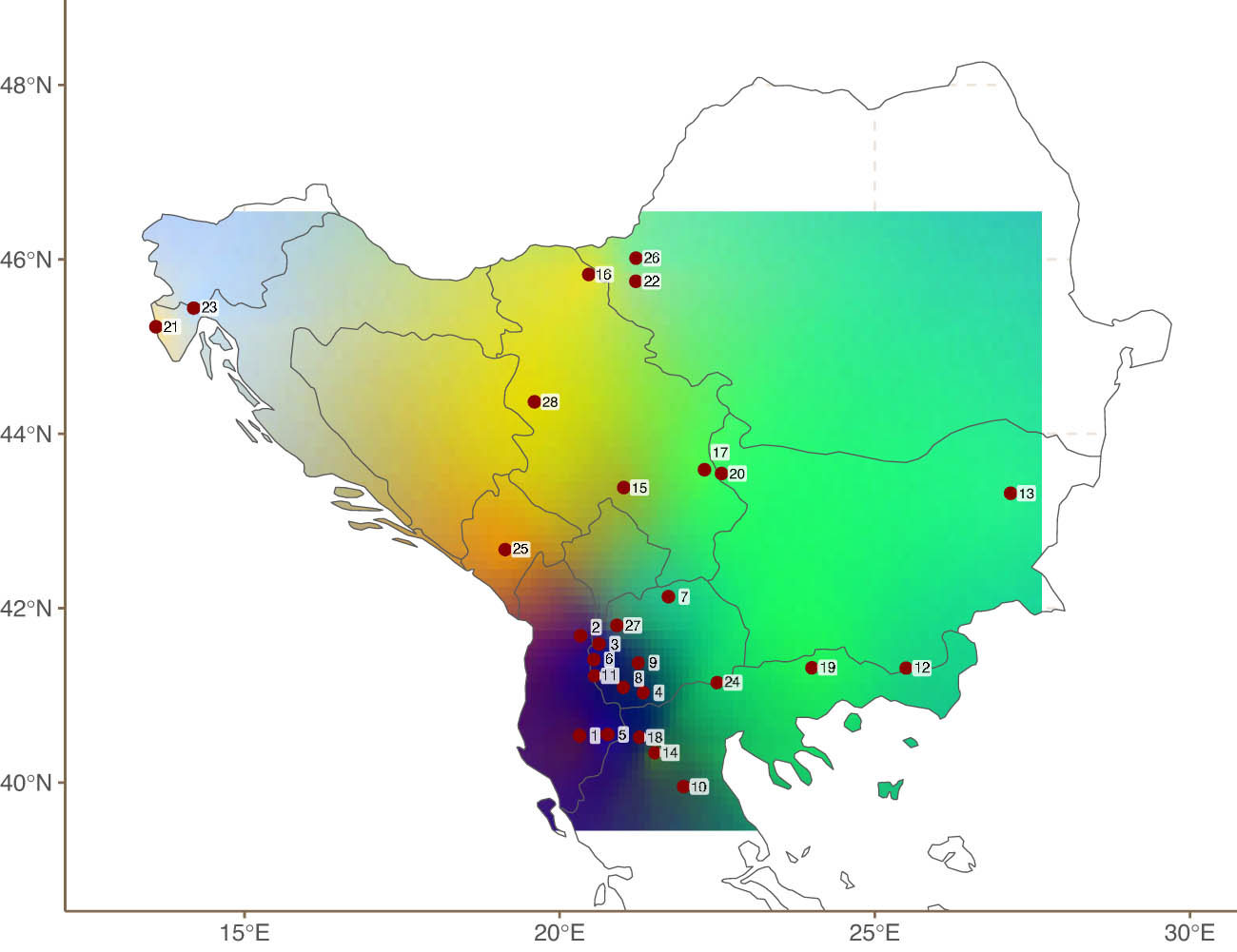
Figure 1 shows the location of the Balkan lects in the data. The dataset contains 28 lects with 48 binarised features (47 before binarisation).[15] The lects in this sample include varieties of Albanian, Bulgarian, Macedonian, Torlak, Serbian-Croatian-Montenegrin-Bosnian, Aegean Slavic, Romanian, Aromanian, Istroromanian, Greek, and Balkan Turkish. It is worth noting that this region is relatively mountainous, with elevations of over 2,900 m. This topography makes use of Euclidean or Haversine[16] distances problematic. Instead, we use topographic distances (see also Guzmán Naranjo and Jäger (2024)) which are the shortest path between two points taking elevation into account. Even though two points might seem to be very close to each other in a two-dimensional space, the presence of mountains can make the actual distance much larger.
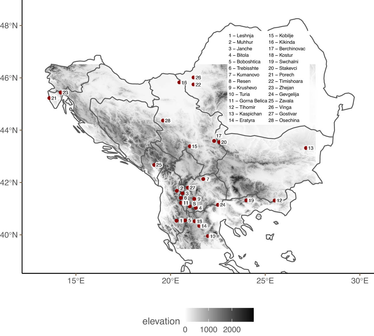
Location Balkan lects.
3.2.2 South American languages
The South American dataset contains 100 languages and 49 binarised features (36 before binarisation).[17] Figure 2 shows the location of all languages in the dataset. As with the Balkan dataset, the topographic features of the region are highly relevant, with some languages being spoken at very high altitudes (see, Urban 2020, Urban and Moran 2021, for a discussion of possible effects of altitude on language). As mentioned earlier, we calculated topographic distances for all languages in the dataset.

Location South American languages.
3.2.3 The Americas
Finally, the dataset for the Americas, originally collected by Urban et al. (2019), contains 77 binary features across 44 languages, spanning from the south of Argentina to the north of Mexico. Figure 3 shows the location of all languages in this dataset. This dataset differs from the South American dataset in two important ways. First, the languages for this dataset are all close to the Pacific coast. Second, this dataset sacrifices density coverage for number of features annotated, and the inclusion of some underdescribed languages. As a consequence, these data have numerous missing data points, 599 out of 3,388 in total (see the Supplementary materials[18]), which should allow us to test our model in an extreme case.

Location American languages.
As with the other two datasets, we calculated topographic distances for all languages in this dataset. Topographic distances in the Americas assume land-based contact only. While we are aware that there was likely some degree of sea-based contact between some of the languages in our data, implementing two types of contacts in the same model is beyond the scope of our study.
3.2.4 Empirically informed priors
Our empirically informed priors for the Balkan and South American case studies are the same as those used by Ranacher et al. (2021) to make our results more comparable. For the Balkans, these are not calculated based on a global sample of languages. Instead, these priors are based on a stratified sample of 19 languages belonging to the Standard Average European (SAE) area, excluding the languages of the Balkans (Haspelmath 2001, Whorf 1956).[19] A significant issue with this approach is that since the SAE is itself considered an area with a high degree of both contact- and family-driven similarity, it is likely to contain a skewed distribution of features compared to a global sample. Thus, rather than reflecting global tendencies in feature universality, these priors represent European tendencies outside the Balkans. For transparency, we will refer to these priors as ‘European’ rather than ‘global’ or ‘universal’.[20]
For the American dataset, we do not have a pre-designed global prior dataset. However, because many of the features used by Urban et al. (2019) are also defined in the World Atlas of Language Structures (Dryer and Haspelmath 2013), we can use WALS to estimate global priors for a good portion of the features in question (39 in total).
Some of the features are not defined in binary terms in WALS. For example, the order of Subject, Object and Verb (feature 81 in WALS) is not binary; instead, it has seven possible values: SVO, SOV, OSV, OVS, VSO, VOS, and Indeterminate. The features in our dataset are defined in binary terms: ‘Is the main order of Verb and Object VO’? In these cases, we took care of binarising the corresponding WALS features.
Since we have relatively large datasets for many of the features, we have two options for estimating the global priors. The easiest one is to build a relatively balanced sample for each feature and estimate the proportion of 1’s in the data. This is the approach taken by Ranacher et al. (2021). The idea is that by building a restricted sample of languages, we control for genetic and areal effects and thus the resulting proportion more or less represents global tendencies. This means that our global priors are, hopefully, not significantly shaped contact or genetic tendencies, but really reflect the global preference for each feature.
An alternative is to keep all the data points and use a predictive model for each feature with phylogenetic and areal controls built directly into the model. We then use the estimate of the intercept (its mean and standard variation) as the prior for our features. This works because the intercept of a model corresponds to the expected value of the feature, when all other covariates are set to 0. By adding phylogenetic and areal controls, we remove most potential biases resulting from either genetic or contact effects, and the resulting estimates should correspond to global tendencies. We follow Verkerk and Di Garbo (2022) and Guzmán Naranjo and Becker (2021) in using a phylogenetic term[21] to control for genetic bias, and we use an approximate GP to estimate the spatial relations in the data (Guzmán Naranjo and Becker 2021).[22] We model each feature independently of each other (i.e. we fit individual models to each feature).[23] Since each model has a phylogenetic and spatial component, we can interpret the intercept as the expected value of a feature once we have controlled for spatial and genetic biases.
To avoid any additional potential effects of contact, we removed all languages from the Americas from the datasets before estimating the global priors, both with the sampling and the model approaches. While it would be possible to keep the American languages non in our sample, we believe the more conservative approach of not considering any American language is the safer alternative in this case. Priors should not be based on the dataset used when fitting the model. If we were to include American languages in the prior calculations, we run the risk of introducing bias priors due to, contact effects between the languages in our sample and languages used for the prior estimation.
4 Results
4.1 Balkans
4.1.1 Cross-validation
We first start by looking at model performance on new data. The idea is that we want to compare different model specifications, and see how they would perform when trying to predict the values of the features of languages not in the dataset used to train the model. The model with the highest accuracy (i.e., the model which best predicts new data points) is the model that best captures the spatial relations in the data. To perform cross-validation, we split our data into ten groups. We then train each model leaving one group of data points out and try to predict the left-out group. We then repeat this process for all ten groups. The model predicts the expected feature value for each feature, for each language.
We compare the quality of the predictions using balanced accuracy. The balanced accuracy is simply the accuracy of the model above what we would expect to get by random chance. This is important because features are not perfectly balanced between 1 (present) and 0 (absent). If, for example, a feature
Table 1 shows the mean balanced accuracy for all models. The model with normal priors is the model without any European prior information, the model with narrow European priors specifies a SD of 0.5 on the empirically estimated priors, and the model with wide European priors has a meta-prior on the SD of the empirically estimated priors. In this case, we observe that the model with empirically informed priors has the highest balanced accuracy of all the models, while the model without family effects performs the worst. We can mention here that the first model in Table 1 (GP + family with normal priors) is effectively multivAreate 1. This is the only instance in which we can directly compare multivAreate 1 with the new version, and we see that the possibility of including external prior information is a clear advantage of the new model.
Accuracy difference European vs normal priors for Balkan lects
| Model | Intercept priors | Mean balanced accuracy |
|---|---|---|
| GP + Family | Normal priors | 0.629 |
| GP + Family | European priors (wide) | 0.625 |
| GP + Family | European priors (narrow) | 0.635 |
| GP | European priors (narrow) | 0.554 |
| GP | Normal priors | 0.551 |
| GP | European priors (wide) | 0.54 |
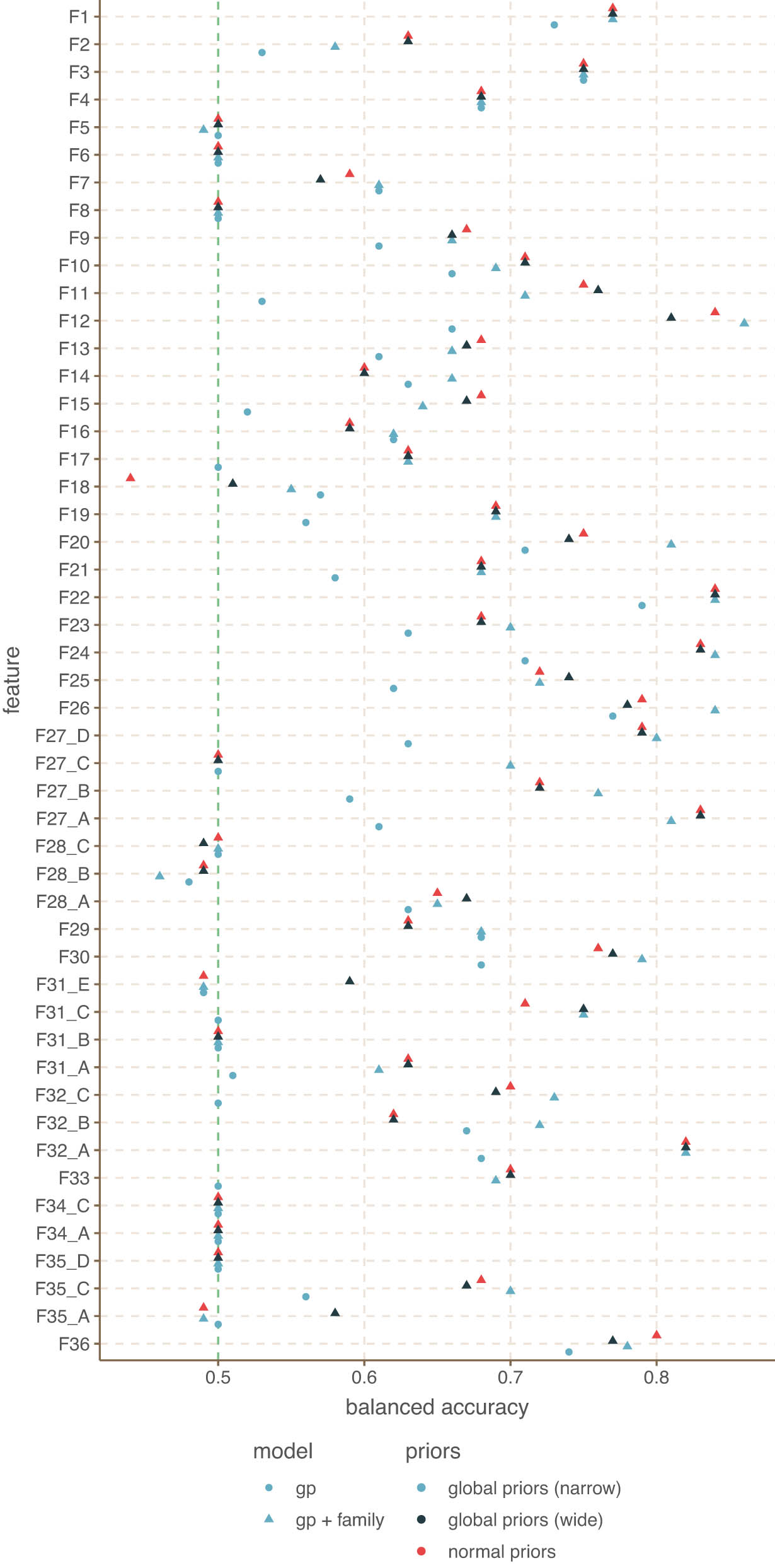
Figure 4 [24] shows the balanced accuracy of the leave-one-out cross-validation. This plot shows the cross-validation results of four models, three with both a GP and family effects, and one with only a GP. For the family effects, we also tested three types of priors on the intercepts: normal priors, global informative (narrow) priors, and global weakly informative (wide, adaptive) priors. The model without family effects has informative narrow priors.[25]

Cross-validation balanced accuracy for Balkan lects.
First, we note that, unlike the spatial patterns shown in the previous section, the predictions of this model can take into account inter-feature correlations. This means that even if there are no clear areal structures, the model might be able to make correct predictions for some of the features and feature values. In addition, the models with family effects can also make use of this information to make predictions.
There are several important observations here. First, multiple features perform at either chance level or below chance level. What this means is that there is not enough information in the data to predict the left out observations above the chance level. When we focus on the model without family effects, this effectively means that the feature in question shows a homogeneous or random spatial distribution. Features like
Second, while the model with narrow priors has a better overall performance, it is not the case that this model performs best for all features. In some cases, other models come out ahead. Even the model without family effects has better performance for F46_0 and F46_1.
Third, the model with narrow informed priors and family effects performs slightly better than all other models, even than the model with wide priors. The implication being that including the informed priors into the model as a strong baseline for the intercepts does tend to improve model performance overall. Thus, we can conclude that the ability of adding European (or more generally, global) priors is a useful modelling tool.
4.1.2 Single-feature spatial patterns
Our approach allows us to examine how the model predicts the probability of a particular feature to change given different spatial locations for individual linguistic features. Since these distributions are highly variable, often reflecting different histories and causes of diffusion, it is worth examining some of them in some detail. To that end, we will discuss a number of the features which show a clear areal pattern.
First, we will show the areal patterns of some features which are not traditionally considered constitutive of the Balkan area (‘Balkanisms,’ as they are often referred to in the literature, e.g. Joseph (2010), Lindstedt (2014, 2000)). We will compare how the use of empirically informed priors affects the estimated spatial effects by displaying these results alongside those with normal priors. Second, we will discuss the areal results for two well-known Balkanisms in the light of the literature. The choice of features to discuss is thus based partly on the results of Section 4.1.1 and partly on insights from the literature. As such, this section is not exhaustive, and plots for all features are provided in the Supplementary Materials.
For the interpretation of these plots, it is important to keep two additional things in mind. First, the predictions in these plots only take into account the intercept and spatial term of the model. This means that the family effects are not taken into consideration, which means that the interpolation effects should only be seen as how the relative probability of feature
Alongside a set of features which are not considered typically Balkan, Ranacher et al. (2021) included a set of linguistic Balkanisms in their data based on the list by Lindstedt (2000). We will discuss two features from this set in the light of the literature: F39 (the presence of a postposed definite article) and F44 (the absence of an infinitive verb form).
An enclitic, postposed definite article is found in the core Balkan languages, including Macedonian, Romanian, Serbian, and Albanian, which is considered a convergent feature of the area (Joseph 2010, 622). Modern Greek, however, contains a preposed definite article, as does Romani (Friedman 2011). This does not rule out a contact-based explanation for the presence of the postposed form in the core Balkan languages, nor does it mean that Greek and Romani must be excluded from the linguistic area; not all Balkan languages must have every linguistic Balkanism, and indeed, this is rare.
Upon comparing the plots in Figure 5, we see that the model with informed priors estimates steeper clines between hills and valleys in the plot. In particular, the area of low probability which encompasses varieties of Serbian-Croatian spoken in Zavala (25), Kobilje (15), Oseschina (28), and (peripherally) Kikinda (16) is more salient than in the plot with normal priors. A second locus of low probability emerges around the Greek variety in Eratyra (14), as expected based on the literature. These areal patterns are actually defined by the absence of a postposed definite article since its presence is relatively common according to the prior. This is in line with the idea that Serbian-Croatian and Greek are ‘peripheral’ members of the Balkan Sprachbund (Joseph 2020, Lindstedt 2016). Indeed, a similar pattern shows up in multiple plots, including Figure 6 and some of those in the Supplementary Materials.

Spatial effects for F39: presence of a postposed definite article. (a) European priors:
Another areal feature of the Balkans is the absence of an infinitive verb form (F44) (Friedman 2011). This is not really an absence as such, but a case of replacement: finite verb forms have replaced the infinitive form to the extent that the infinitive has fallen out of use entirely. This process of replacement took place in Greek during Medieval times, spreading from the urban centre of Thessaloniki to other cities, including Athens, Heraklion, Constantinople, etc. (see Joseph 1999, for a detailed account). Thessaloniki was highly multilingual, with close contact between speakers of several languages, including ones which we now classify as ‘Balkan’, such as Albanian and varieties of southern Slavic like Macedo-Bulgarian. This multilingualism likely facilitated innovations in the language through processes such as imperfect language learning and analogy. Moreover, Greek was a prestige language and its urban variants were likely more prestigious yet; thus, speakers of Greek as well as other languages may have borrowed examples of infinitive replacement from specific phrases used by the urban speakers who innovated the new constructions, which were then extended to other contexts through analogy (Joseph 1999, Joseph 2010, Sandfeld 1926).
While this discussion pertains to a very specific form of infinitive replacement, the prior (
As in Figure 5, the strongest areal signal for the absence of this feature encompasses the Serbian-Croatian lect of Zavala (25), but in this case, the areal pattern extends southwards towards Balkan Turkish (27) and an Albanian lect in Muhhur (2). There is also a strong signal involving a Serbian-Croatian lect spoken in Kikinda (16) and Romanian as spoken in Timishoara (22). The lects of Porech (21) and Zhejan (23) are vaguely connected with the previously mentioned northern cluster of languages in that they also show a lower probability of the feature (and indeed, these languages have not undergone infinitive replacement).
The plot with normal priors shows a similar set of areal patterns. This plot allows us to see an area of high probability encompassing the Greek lect Eratyra (14) and a cluster of geographically contingent languages: the Albanian of Leshnja (1), Aromanian of Turia (10), and Macedonian of Boboshtica (5) and Kostur (18). This concentration of high probability towards the south of the Balkan area is expected, since the innovation is posited to have spread from Greek, as discussed earlier (Joseph 1999).
4.1.3 Aggregated spatial patterns
So far we have only discussed the spatial effects for individual features, but we would also like to get a sense of the general spatial structure across languages. We will focus on the model with European priors exclusively for this section, but plots for the model with normal priors are provided in the Supplementary Materials.
Since sBayes focuses on finding general spatial patterns, it is worth starting with the results from their model. Figure 7 replicates Figure 6 in the original article.[27] This will work as a reference, but two observations are worth noting. First, there is a surprising spatial structure in the north, namely, the spatial connections (‘contact area’ as the authors call it) between the lects of Zhejan (23) and Timishoara (22); and the connection between the lects of Porech (21) and Osechina (28). These relations seem unlikely a priori because they require ‘jumping over’ lects. In both cases, it seems likelier that genealogical structure in the form of Indo-European subgroups is driving the similarity between these lects (Slavic in the case of the lects of Porech (21) and Osechina (28), and Romance in the case of the lects of Zhejan (23) and Timishoara (22)).

Spatial effects for F44 (absence of infinitive: true, false). (a) European priors:

Spatial patterns of sBayes for Balkan lects.
Following Guzmán Naranjo and Mertner (2023), we first present the spatial correlations of our model. Since we have independent spatial correlation structures for each feature, here we will only show the strongest and weakest structures. Figure 8 shows the weakest, strongest, and mean spatial correlation structures. What these plots show is the potential correlation due to contact or diffusion that the model can find between two languages. That is, a spatial correlation of 0.5 does not mean that there is in fact contact between the two lects in question, but rather, that there could be a relatively strong spatial correlation between the two lects in question. In contrast, a spatial correlation between two locations that is close to 0 means that the model finds no evidence for any type of contact or diffusion between those locations. This is an important point. The spatial correlation structures are not necessarily evidence for contact, but can be evidence against contact explanations.[28]

Spatial correlation structures of the model for Balkan lects. (a) Weakest spatial correlation structure, (b) strongest spatial correlation structure, and (c) mean spatial correlation structure.
Figure 8(a) and (c) are particularly interesting because these already show a stark contrast with the results in the study by Ranacher et al. (2021) shown in Figure 7. Specifically, there is no spatial correlation between the lects of Porech (21) and Zhejan (23) and the other lects. Even when we look at Figure 8(b), the potential spatial correlation between these two lects and other lects is very weak. Another difference between multivAreate 2 and sBayes is that the potential correlation between the lects of Stakevci (20) and Kaspichan (13) is very weak in ours.
Next, we try two new approaches to combine the information contained on the spatial effects of each feature in the model. First, we aggregate the spatial effects of all features. To do this, we start with a simple transformation. Consider the case of two different features, F1 and F2, which are perfectly anti-correlated: if F1 has value 1 for some observation, F2 has value 0. The individual areal patterns of these two features would be equivalent, but simply adding them or averaging them would result in a null pattern since they would cancel each other out. What matters is not the absolute value for a point, but rather the change of value from one point to another. To capture the contrast between regions, we scale and centre the spatial effect of each feature and then take its absolute value. We then add the transformed spatial effects for all areas, and scale the result to between 0 and 1 for plotting.[29]
The second technique consists of doing image analysis on the areal effects. We perform edge detection[30] on each effect plot and then aggregate the edges across all features. Edge detection basically finds the transition points between areas, effectively finding the places where there are contact barriers. Overlaps will produce stronger edges. For both plots, we have overlaid the elevation data for comparison.[31]
There are some clear overlaps between the results of these two approaches. First, and most apparently, the separation between the lect of Porech (21) and the lect of Zhejan (23) is clear in both figures. Figure 9(a) shows a dip between the lects, while Figure 9(b) has a very strong edge separating both lects. Other points of convergence are the separation between Leshnja (1) and other lects, the separation of Kikinda (16) from Vinga (26) and Timishoara (22), and the separation between Zavala (25) and Kobilje (15). Similarly, we see a relatively strong separation between Kaspichan (13) and Tihomir (12) in both plots.

Unified spatial structures for Balkan lects. (a) Aggregated areas and (b) extracted barriers.
Two of the strongest areal signals in Figure 9(a) have their focus in the south, one around Leshnja (Albanian) (1) and another encompassing Gostivar (27), Janche (3), Trebisshte (6), Gorna Belica (11), and Bitola (4), which are the locations of several languages which are generally agreed to be core members of the Balkan linguistic area. The Greek lect spoken in Eratyra (14) is also somewhat included in the area, though with a slight dip in probability, which makes sense given the somewhat uncertain state of Greek within the Balkans Joseph (2020).
To evaluate whether these areas correspond to actual linguistic differences found in our data, we can calculate the distance between some of these lects based on their feature values. Binary distances between the relevant sets of lects is shown in Figure 10.
First, the separation between Porech (21) and Zhejan (23) seems to be valid, and also in agreement with sBayes. A notable difference between our results and that of Ranacher et al. (2021) is that we find a strong separation between the lect of Gostivar (27), and those of Zavala (25) and Kobilje (15). Indeed, Figure 10 confirms that linguistically, the lect of Gostivar (27) is very different from those of Zavala (25) and Kobilje (15). What seems to be happening in sBayes is that because Gostivar (27) is also very different from other nearby lects like the one in Muhhur (2), and because the model has to assign the language to one of the three groups, it assigns it to the least unlikely of the groups. This, it seems to us, is a weakness of sBayes.

Linguistic correlation between lects.
Another point of difference between our model and sBayes is that we find barriers between the lects of Stakevci (20), Săchanli (19), Tihomir (12), and Kaspichan (13) (of different strengths), while sBayes groups these into the same contact area. However, Figure 9(a) and (b) disagree slightly. While the aggregated areas suggest that the main split occurs between the lects of Stakevci (20) and Săchanli (19) vs those of Tihomir (12) and Kaspichan (13), the edge detection approach finds a strong barrier between Tihomir (12) and Kaspichan (13). Based on the linguistic distance between lects, the latter seems more likely. Indeed, Figure 10 shows that these lects are similar to each other; however, we need to keep in mind that they are all Slavic lects and that much of their similarity likely springs from this fact. Thus, it is unclear whether sBayes is finding a real contact structure, or whether it is not able to fully distinguish between family effects and contact effects. Our model suggests that the contact relations in this region are not as straightforward, and that a good portion of the variance can be attributed to family effects.
From Figure 10, it is also easy to see why sBayes finds connections between Porech (21) and Osechina (28), and Zhejan (23) and Timishoara (22): linguistically, these pairs are very similar. Our model, however, cannot find discontinuous connections which require jumping over other observations. That is, we cannot model a contact relation between
4.2 South American data
4.2.1 Cross-validation
We start again by comparing model performance on new data. Table 2 shows the average accuracy for each of the four models for South American languages. As with the Balkan dataset, the model with narrow global priors and control for family effects performed better than the rest, and the model without family controls performed worst. Unlike the empirically informed priors for the Balkan dataset, the global priors for this case study were informed by a stratified sample of languages from across the world. This means that these priors should reflect global tendencies for the presence or absence of each feature.
Accuracy difference global vs normal priors for South American languages
| Model | Intercept priors | Mean balanced accuracy |
|---|---|---|
| GP + Family | Normal priors | 0.653 |
| GP + Family | Global priors (wide) | 0.657 |
| GP + Family | Global priors (narrow) | 0.666 |
| GP | Global priors | 0.592 |
Figure 11 presents the balanced accuracy for each feature in the South American language dataset.
Cross-validation balanced accuracy for South American languages.
4.2.2 Spatial patterns
Figure 12 is a replication of Ranacher et al. (2021)’s results for South America.[32] In contrast to the results for the Balkan lects, the model finds that most languages in South America do not belong to any contact area (those languages are represented by dots in grey). Moreover, contact areas 1 and 2 extend over very large areas and connect languages which are located extremely far apart. These are extreme situations of jump-over contact effects, which we find difficult to interpret. Perhaps the most notable result of this model is that it finds such faraway connections, but does not seem to infer contact between several languages which are geographically close together.
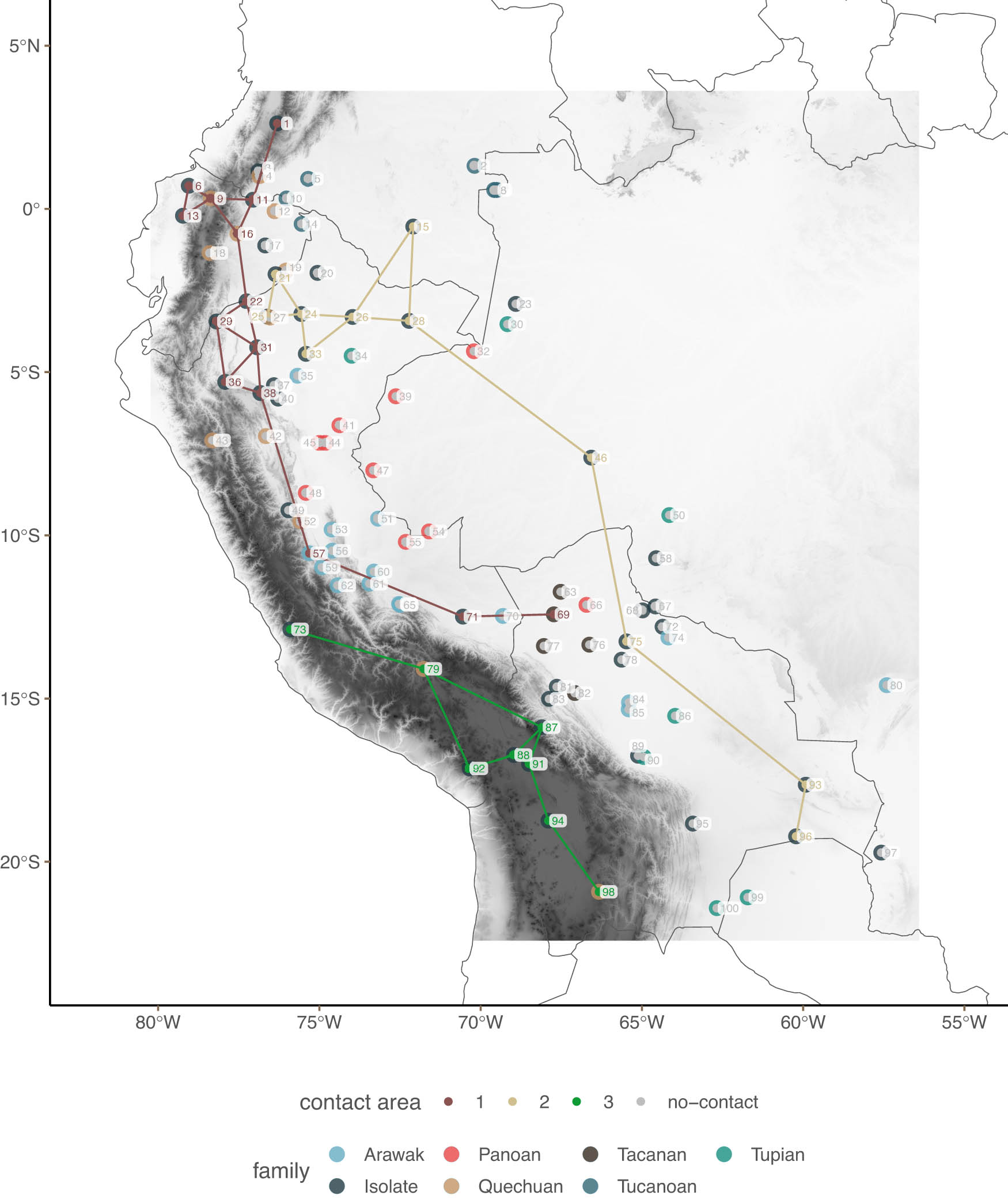
Spatial patterns of sBayes for South American languages.
For reasons of space, and because the spatial structures in South America seem to be more complex than in the Balkan data, we will focus exclusively on the effects of the model with global (narrow) priors and will not discuss or compare the effects of the model without global priors.[33]
First, Figure 13(a) (presence of phonemic uvulars and velars) shows a relatively strong Andean vs non-Andean language separation, similar to the one claimed by Ranacher et al. (2021). However, what we do not see is that this area extends all the way above Ecuador and to Colombia. Moreover, the areal pattern extends (more weakly) well into Bolivia and possibly Brazil. This issue becomes more apparent in Figure 13(b) (presence of phonemic aspirated consonants), which displays a barrier along the Peru-Ecuador border. Figure 13(b) also shows that large-scale areal patterns are in some cases made up of smaller clusters and not necessarily very large extended areas.
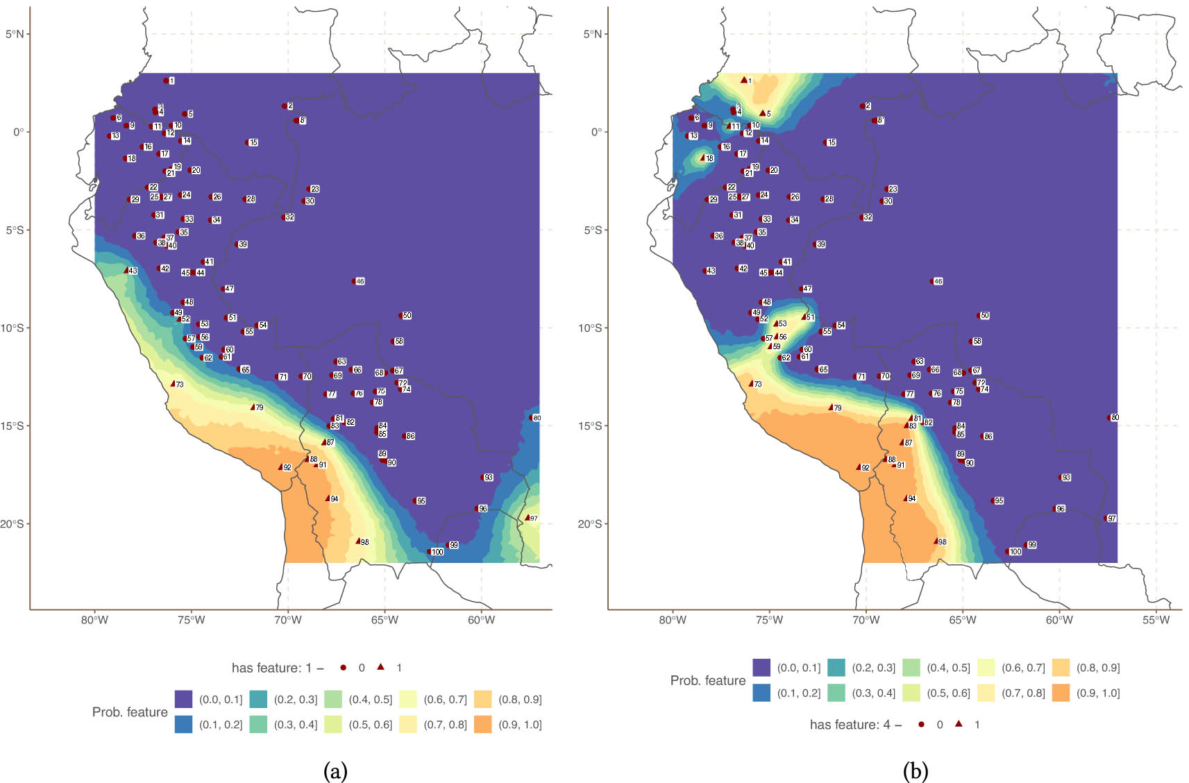
Spatial effects for features F1 and F4. (a) Spatial effects for feature F1 (uvulars and velars) and (b) spatial effects for feature F4 (aspirates).
Figure 14(a), showing the distribution of aspirated stops, shows once again an areal structure in Andean languages in southern Peru and northern Chile, as well as Bolivia, but this pattern is supported by relatively few observations and stops before reaching the Peru-Ecuador border. Feature F6 is the presence of ‘more phonemic affricates than fricatives’, which Aikhenvald (2007) associated with Amazonian languages. However, Urban (2019), drawing on a broad sample of languages not belonging to the Quechuan or Aymaran families, argues against the claim that Andean languages tend to be less affricate rich. Thus, the areal pattern in our map reflects the relatively rarity of this feature in the Andes overall, and the fact that the languages which do have it are not necessarily related. The inferred area encompasses the area where Chipaya (94) is spoken, as well as Bolivian Quechua (98) and (in the periphery of the area) Aymara (91), Muylaq Aymara (92), and Uru (88). Indeed, then, this is a phylogenetically diverse area, as three languages families meet here: Uru-Chipaya, Quechuan, and Aymaran (Torero 2002, Adelaar 2012).

Spatial effects for features F6 and F7. (a) Spatial effects for feature Feature F6 (more phonemic affricates than fricatives) and (b) spatial effects for feature F7 (phonemic bilabial and labial fricatives).
Another areal structure which clearly appears in this figure is the one in the centre, mostly in Brazil, where languages clearly lack the feature in question. Figure 14(b) (the presence of bilabial and labial fricatives) is interesting because it shows highly localised areal patterns, as well as some structures in Brazil and Bolivia. Most importantly, we see again a pocket in southern Colombia and northern Ecuador which behaves quite differently from its surrounding languages, and other Andean languages.
We will now focus on the aggregated spatial patterns.
As mentioned earlier, the images under Figure 15 show the potential spatial correlation structures between languages for the models in question. If two languages are not connected in these plots, it means that they cannot influence each other in the model. If two languages are connected, it means they can, but not necessarily that they do. There are several important observations here. First, sBayes suggests a connection across the Amazon for the languages Yagua (28) and Jarawara (46). However, this connection is barely visible in Figure 15(b) with a correlation of about 0.01. The spatial correlation between these two observations is effectively 0 in the mean case in Figure 15(c). A similar situation can be seen for the predicted connection between Chayahuita (38) and Yanesha’ (57) which is effectively 0 for all correlation structures (0.03 for the strongest). The same can be observed for connections between Jarawara (46), Cayubaba (75), and Chiquitano (93), which all lie below 0.03 in the strongest spatial correlation structure.

Spatial correlation structures of the model for South American languages. (a) Weakest spatial correlation structure. (b) Strongest spatial correlation structure. (c) Mean spatial correlation structure.
Anticipating also some results of the joint evaluation of all features that we move to now, what our model suggests is that language contact in South America is to a significant degree an affair of contact between close languages, perhaps within regional systems as outlined in Epps (2020), and larger patterns the product of different effects, perhaps related to expansion and/or ‘water bucket’ phenomena in which large patterns emerge from multiple short-distance contact situations.
Figure 16 shows the combined spatial effects of all features, as well as the combined extracted edges.

Unified spatial structures for South American languages. (a) Aggregated areas. (b) Extracted barriers.
We find three interlocking zones of high spatial correlation, all centred in the lowlands to the east of the Andes: (1) the Upper Amazon of Ecuador and Peru, (2) the lowlands of central Peru, on both sides of the Ucayali river, and (3) the lowlands of northern Bolivia around the Beni and Mamoré rivers. In the results of the model, the sparsely sampled Andean languages align with their lowland neighbours at the respective latitudes rather than showing strong evidence of correlation among themselves. Like in the results of Ranacher et al. (2021), these are connected to one another, though the improved model shows stronger evidence for regional clusters of languages, perhaps reflecting regional rather than long-distance patterns of interaction.
Indeed, parts of the qualitative literature are consistent with this: the Upper Amazon region, in particular along the lower course of the Marañón river, is an area of complex linguistic dynamics. The presence of far western outliers of major language families, such as Cocama (Tupian) and perhaps Patagón (Cariban) along the course, suggests a history of westward language expansion (Urban Forthcoming, Urban et al. Forthcoming). While much is still to be understood, Cocama in particular seems to have a history of profound interaction and contact, and perhaps creolisation, involving one or more other Indigenous languages (e.g. Cabral 1995, 2000, Bakker 2020). But evidence for contact is not restricted to this language. Cahuapanan influence on the Muniche language in phonology and lexicon are discussed by Michael (2013, 339–40), and while some aspects of the data do not support the idea as unequivocally as Rojas-Berscia and Eloranta (2019) suggest, there is qualitative evidence for language contact from grammatical subsystems and perhaps shared grammaticalisation involving not just bilateral contact, but several languages of the region.
In the central part of Peru, Huallaga Quechua (52), Cholón (49), Yanesha’ (57), and Arawakan languages of the so-called Campa branch, as well as Panoan languages such as Cashibo (48), Amahuaca (55), and Yaminahua (54), participate in a network of increased spatial correlation structure. The qualitative literature describes why this may be so in terms of language contact: The most well-known and well-researched case of language contact is that between Yanesha’ (57) and Quechuan. Yanesha’, an Arawakan language, has been phonologically literally transformed under Quechuan influence and has received loanwords not only from a Quechua II variety that give the impression of having arisen in imperial contexts and is associated with male-biased gene flow from the highlands Barbieri et al. (2014) but also from local varieties of Quechua I that may have arisen in a quite different and likely more egalitarian context. These effects are described in most detail in Adelaar (2006) seminal article; the contacts of Yanesha’ (57) have been likely more complex than a bilateral situation as there is evidence for the signature of a further, unidentified language in Yanesha’ (57) as currently spoken (cf. Muysken 2012, 240). But also some of the Campan languages seem to have been influenced by their proximity to the highlands and its languages; van Gijn and Muysken (2020, 190) attribute the loss of mid-vowels in Ajyiiininka Apurucayali (53, and Yanesha’) to that; and Mihas (2017, 786) ponders whether the presence of aspirated stops and affricates in Campan can be attributed to contact with Quechuan, which, as we have seen, are relatively rich in the latter. Finally, Cholón (49) is a language that has a contact history with Quechuan (Muysken 2012, 239–40), but likely also other languages of the regional linguistic system in which it was embedded Urban (2021).
Finally, we observe a large network of languages with high spatial correlation in the lowlands of Bolivia, which extends into the Andes of Southern Peru. The lowland part corresponds, to a large extent, to the so-called Guaporé-Mamoré linguistic area’ proposed first by Crevels and van der Voort (2008), and our results are particularly important since Muysken et al. (2015b) were only able to reproduce the picture as painted by Crevels and van der Voort (2008) by selecting features manually, but not upon a bottom-up approach that takes into account an array of features not selected a priori because they show evidence for convergence in the area. The fact that we can do so through our model lends support to the claim of convergence effects (though we believe that a lot of more fine-grained research into the linguistic history of the area is necessary at this point).
The Andean part of this network is less well pronounced in our results, though it is known particularly well as a region of intense language contact involving four different language groups: Quechuan, in particular the branch called ‘Quechua IIC’ or ‘Southern Quechua’, Aymaran, in particular the varieties of Aymara itself, Uru-Chipaya, and Puquina. Evidence for language contact is decisive and involves extensive lexical borrowing, including core and cultural vocabulary; widespread borrowing of bound derivational morphology; semantic isomorphism of the function of derivational morphology (compare for these points e.g. Cerron-Palomino (1994), Adelaar (1986, 1990), Torero (1992) and the descriptions in Cerron-Palomino (2006), Emlen et al. (Forthcoming), Hannß (Forthcoming)), and, under one of the possible accounts, phonological innovation in Quechuan of a series of aspirated and ejective consonants under Aymaran influence (see e.g. Torero 1964, Mannheim 1991, Landerman 1994, Campbell 1995), for a skeptical view.
The qualitative evidence for the link between the Andes and the Bolivian lowlands that we see in our results is somewhat weaker, though that may reflect a dearth of research at this point. There is evidence for contact between highland languages and lowland languages like Mosetén that is evidenced in shared lexical material having to do with culture (Pache et al. 2016, Adelaar 2020, Zariquiey 2020), in shared views of numeracy and ways of counting that also involves lexical transfer (Pache 2018) and some structural resemblances indicative of contact or perhaps deep ancestry (Adelaar 2020).
Two salient differences between our results and those obtained by Ranacher et al. (2021) lie in the shapes of the contact areas we observe. They find two latitudinally structured contact areas in the central and southern parts of the Andes, and an even larger one along the eastern slopes that runs from the Andes from Ecuador through Peru and into Bolivia.
While their results for the Andes are compatible insofar as we do see the high-contact area in and around the altiplano of southern Peru and Bolivia reflected in our results as well, it differs in that, in our results, Jaqaru – Aymara’s sister language within the Aymaran language family – is not part of this network, and that it is linked to the lowlands via Leco and Mosetén in particular as ‘gateways’. These results do make sense insofar as indeed the location of Jaqaru in the highlands of Central Peru places it outside of the circum-altiplano contact sphere, and that, as discussed earlier, there is lexical and grammatical evidence for highland–lowland contact. While we do not wish to over-interpret the results, these may be indications that the model underlying this study is better capable of identifying contact-induced similarities and distinguishing them from genealogical inheritance such as that which links Jaqaru and Aymara.
On the other hand, while in our results, the languages involved in Ranacher et al.’s Z1 area are also connected, the spatial structure of the correlations is more suggestive of three cloud-like clusters in the Upper Amazon, central Peru, and the Bolivian lowlands as discussed earlier. Even though Ranacher et al. (2021) do not mention this, the qualitative literature precisely contains hints that suggest convergence specifically among the languages of the eastern slopes that has the same longitudinal structure as observed by them Wise (2011), Valenzuela (2015). This is not clearly reflected in our results, however.
4.3 The Americas
This case study is slightly different from the previous two case studies because we are not trying to replicate a previous result of sBayes, but to stress-test multivAreate 2 in a case with an extreme number of missing values and a very large number of features. For this reason, we do not explore as many model combinations as in the previous case studies. The first observation is that despite the large number of missing data points in the dataset, the model had no trouble in terms of computation. From a model fitting perspective, there were no convergence or transition issues. This shows that multivAreate 2 can handle datasets with large numbers of missing data points without difficulty.
4.3.1 Cross-validation
For this case study, we only focus on two models: one fitted with priors based on a stratified sample of WALS (sampling-based priors), and one model fitted with priors based on individual models for each feature using the whole dataset available in WALS minus the American languages (model-based priors). Figure 17 presents the leave-one-out cross-validation process applied to the American dataset.
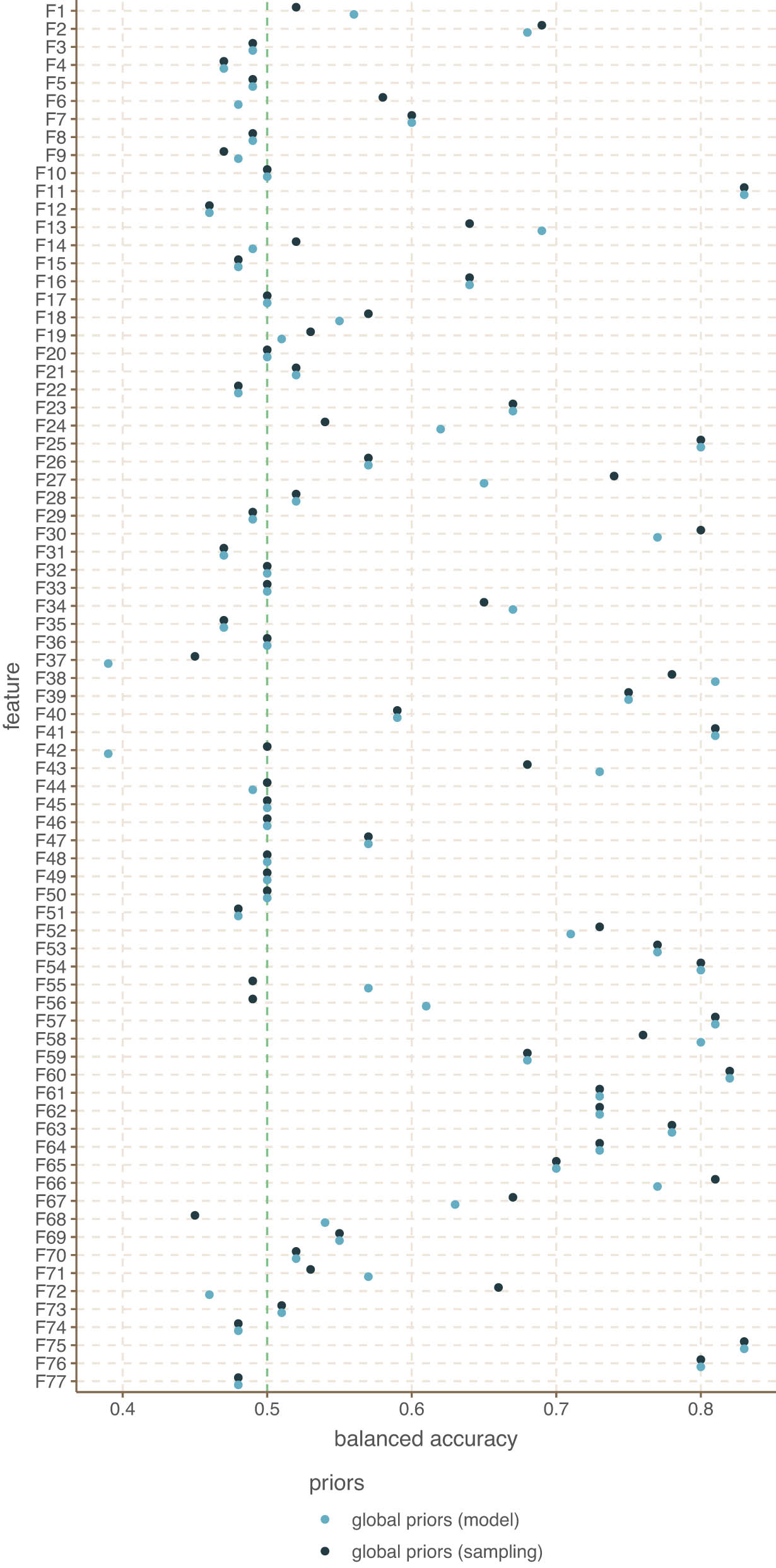
Cross-validation balanced accuracy for American languages.
The average accuracy by model is shown in Table 3. Both approaches to estimating priors are very close to each other, with the model-based priors faring slightly better. Overall, there does not seem to be much improvement from using model-based priors over simpler sampling-based priors.
Accuracy difference prior specification for American languages
| Model | Intercept priors | Mean balanced accuracy |
|---|---|---|
| GP + Family | Global priors (sampling) | 0.6 |
| GP + Family | Global priors (model) | 0.61 |
4.3.2 Spatial patterns
Figure 18 shows the minimum, maximum, and mean spatial correlation structures for the American dataset. There are several important things to note. First, even though we allowed the model to find much longer distance correlations, there do not appear to be any above a few hundred kilometres. The mean value for the length-scale parameters is 2.22, which is very close to 1.49, we found with the South American dataset, and which restricts contact effects to a few hundred kilometres (up to about 450 km). Even for the feature for which the model found the largest length-scale, we do not see clear evidence of long-distance contact. This is important because languages of the South American Pacific coast like Mochica and Esmeraldeño have been observed to exhibit salient typological similarities with language families of South America. This observation has been attributed to possible Mesoamerican long-distance contact, and the impressionistic assessments as to typological similarities in the qualitative literature have in fact been confirmed quantitatively on the basis of the dataset also used here (Urban et al. 2019). The results obtained here, however, suggest that this proximity is due to factors unrelated to direct long-distance contacts in prehistory.
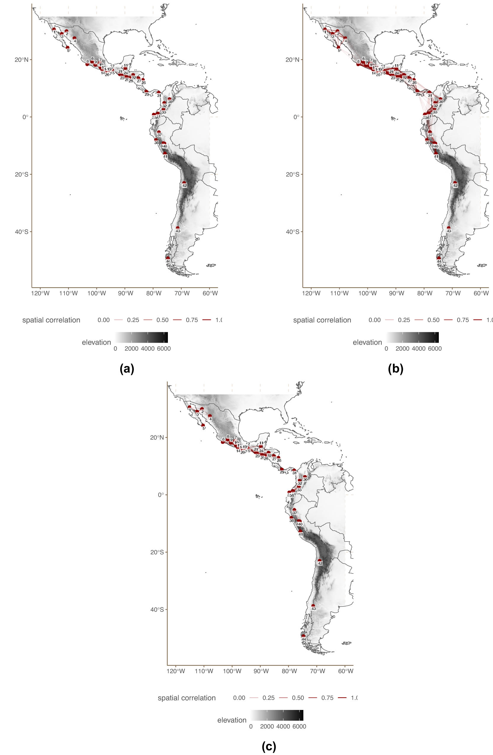
Spatial correlation structures of the model for American languages. (a) Weakest spatial correlation structure. (b) Strongest spatial correlation structure. (c) Mean spatial correlation structure.
If there was evidence for long distance contact effects, we would expect to see a mean correlation plot with longer, and stronger, correlations than what we see for the strongest spatial correlations in Figure 18(b). The current model only finds as potential South America-Central America contact some weak correlations between languages in southern Colombia/northern Peru and languages in Panama. There is no evidence for long distance Pacific contact relations.
Similarly, and consistent with the results, we obtained for the South American dataset from Ranacher et al. (2021), our results suggest that larger scale typological patterns across the South American continent are not likely induced by language contact on a commensurately larger scale. In this vein, Urban et al. (2019) observed a hitherto unnoted typological gradient in the western (mostly Andean) part of South America. As they noted, this spatially structured typological variation could either be the net cumulative result of multiple small-scale, more localised contact events that result from the long-term interaction of speakers of neighbouring languages, or it could possibly reflect a signal of linguistic history that is different from contact. As already noted by Urban et al. (2019), there is indeed no scenario derivable from what is known on the prehistory of the South American continent that would plausibly involve language contact over virtually its entire north-south axis, suggesting that the pattern may reflect older demographic processes relating to the expansion of humans across the continent.
5 Conclusion
In this article, we have reviewed how the models proposed by Ranacher et al. (2021) and Guzmán Naranjo and Mertner (2023), which both offer several interesting innovations for the statistical detection of language contact and linguistic areas. We also discussed the advantages and disadvantages of both methods, and suggested that we should combine their advantages. To do this, we have proposed an improvement on the model by Guzmán Naranjo and Mertner (2023), multivAreate 2, which solves most of its predecessor’s shortcomings and integrates sBayes’s innovations.
The key properties of this improved method are the following: (1) it can handle highly correlated binary data, and account (control) for that correlation, (2) it can handle and impute missing data, (3) it can produce interpolation maps, (4) it can make predictions on new data, and (5) it can be easily integrated into larger generalised regression models. This is a clear improvement on both sBayes and multivAreate as presented by Guzmán Naranjo and Mertner (2023).
By using multivAreate 2, we explored three datasets: the Balkans, western South America, and a more general, sparse dataset for the Pacific region in the Americas. We find that the model correctly captures multiple areal patterns that have been suggested in the literature, but in ways that sometimes differ drastically from alternative extant approaches. For the Americas, the model does not find much support for large-scale contact events along the Pacific coast; instead, we see what is likely the outcome of many contact events at shorter distances. Similarly, for the Balkans, our model finds little support for long-distance contact, instead finding local areas of convergence which together result in the observed areal patterns at the macro-level.
One open question is that of jump-over effects, or contact between languages which are not geographically contingent or where there are other languages between them. As discussed with respect to the Balkan and South America datasets, sBayes finds jump-over effects even if there is no clear evidence that they are indicative of contact. The issue is that sBayes does not have any deeper knowledge about the history of the contact situation, resulting in situations where deep-time phylogenetic relationships may be misclassified by the model as contact. Properly implementing jump-over contact effects is extremely difficult. The model would need to be able to distinguish between real and apparent jump-over situations, which is a non-trivial problem. sBayes consistently finds apparent jump-over effects, while multivAreate never does. We think that the multivAreate approach is the safer alternative, given that we cannot reliably exclude incorrect jump-over situations. Ultimately, how to reliably implement jump-over effects in multivAreate will have to remain an open question for now.
One methodological possibility which we did not explore or discuss in this article is that multivAreate 2 can be easily expanded to handle other types of data along with binary data. Since the model is based on an underlying Multivariate Normal distribution, it is possible to also include continuous variables, as well as ordinal variables.[34] For example, one could include socio-cultural variables which can be modelled as approximately normal, and which may be correlated in a non-causal way with other linguistic features. Alternatively, some count features like number of segments could be modelled as approximately normal and correlated with other binary features. Another methodological innovation which could be integrated into our model is the use of informative priors for the correlation matrix. The same way we add universal priors to the intercepts of the features, we could calculate universal correlation priors across the features in question and add these to the model. We leave these issues for a future article.
-
Funding information: Matías Guzmáan Naranjo received funding from the German Research Foundation (DFG, grant no. GU 2369/1-1, project number 504155622). Miri Mertner received funding from the European Research Council (ERC) under the European Union’s Horizon 2020 research and innovation programme as part of the project ‘CrossLingference’ (grant agreement 834050). Matthias Urban received funding from the German Research Foundation (DFG, grant no. UR 310/2-1) and the European Union (ERC, LANGUAGE REDUX, project number 101124345).
-
Author contributions: All authors have accepted responsibility for the entire content of this manuscript and consented to its submission to the journal, reviewed all the results and approved the final version of the manuscript. Matías Guzmán Naranjo: conceptualization, statistical modelling, writing. Miri Mertner: conceptualisation, background information, linguistic analysis, writing, and Matthias Urban: data collection, linguistic analysis, and writing.
-
Conflict of interest: The authors state no conflict of interest.
-
Data availability statement: All code and data are available at: https://osf.io/73nrb/?view_only=a6c881a0c89d4e05932873f5c758ccb9.
Appendix A Mathematic description of multivAreate
The basic definition of multivAreate is as in equation (A1). In this definition
The spatial component is handled by the GP, here
For adding global priors, we just need to modify the priors on
Finally, the lines starting with
Definition of multivAreate.
We want to note here that the likelihood is implemented in Stan in a very different way than the simple definition above. The implementation is in the functions block in the Stan model code. These differences have performance reasons (similarly to how most linear algebra operations have implementations that do not reflect the way people understand them). But the aforementioned model is an accurate description of what is going on conceptually.
B Alternative aggregation methods
B.1 Balkans
In this section, we present two alternative, more traditional methods for aggregating the conditional effect structures. In the main text of this article, we introduce two new techniques, one based on effect aggregation, and one based on border detection. Here, we show a clustering method and an RGB method.
Figure A1 shows the hierarchical clustering based on the individual conditional effect plots. We present plots for two to nine clusters. We chose these ranges because at nine clusters we start to see regions emerge without any data points in them. These clusters match very closely to what we saw in the article: a clear south-central region of high contact, a separation along the middle line between east and west, and a possible separation between the lects 19 and 12 from 13. This separation only appears in the clustering approach at nine clusters, suggesting that it is not very strong. The first split at two clusters divides the centre-east region from the north-western region, suggesting these two areas show the most divergence.

RGB compression of the conditional effects for the Balkans.
Figure A2 shows the RGB compression Nerbonne et al. (1999) of the individual conditional effects plots. We created this representation by taking the principal component analysis of the conditional effects for all features, and picking the 3 main components. We then mapped each component to a Red, Green and Blue value, which we then converted into a hex colour value. The absolute colour does not represent any specific value, but locations with similar colours should be linguistically similar according to the spatial component of the model. In this representation, we pick up most of the same spatial structures as in the other plots: We see a separation in the centre region and a strong cluster in the south-central region. The Western region also shows a clear difference from the other regions.
Hierarchical clustering based on conditional effects for the Balkans.
B.2 South America
Next we look at South America. Figure A3 shows the hierarchical clustering of the conditional effects, and Figure A4 shows the RGB compression. As with the Balkans in the previous section, these representations mostly agree with each other and with the representations in the main text. We see very similar region spanning the Andes and in the Amazonas. A difference in this case is that the edge detection for the South American data did not produce very clear borders, but the RGB structure does seem to indicate that there are some clear linguistic borders. The most important point, however, is that we do not see (as in the main text) any indication of very large contact scenarios, rather we find only short-scale contact between languages.

Hierarchical clustering based on conditional effects for South America.

RGB compression of the conditional effects for South America.
Ultimately, be it edge detection, clustering, effect aggregation or RGB compression, it is important to interpret the results of the models with respect to the literature, and keeping in mind known areal structures and contact situations.
References
Adelaar. 2012. “Languages of the Middle Andes in Areal-Typological Perspective: Emphasis on Quechuan and Aymaran.” In The Indigenous Languages of South America, edited by Lyle Campbell and Verónica Grondona, 575–624. De Gruyter. 10.1515/9783110258035.575.Suche in Google Scholar
Adelaar, Willem F. H. 1990. “Aymarismos en el Quechua de Puno.” Indiana 11: 223–31. Suche in Google Scholar
Adelaar, Willem F. H. 1986. “La relación quechua-aru: perspectivas para la separación del léxico.” Revista Andina 4 (2): 379–426. Suche in Google Scholar
Adelaar, Willem F. H. 2006. “The Quechua impact in Ammuesha.” In Grammars in Contact: A Cross-Linguistic Typology, edited by Alexandtra Y. Aikhenvald and Robert M. W. Dixon, 290–311. Oxford: Oxford University Press. Suche in Google Scholar
Adelaar, Willem F. H. 2020. “Linguistic connections between the Altiplano region and the Amazonian lowlands.” In Rethinking the Andes-Amazonia divide: A Cross-Disciplinary Exploration, edited by Adrian J. Pearce, David G. Beresford-Jones, and Paul Heggarty, 239–49. London: UCL Press. 10.2307/j.ctv13xps7k.26Suche in Google Scholar
Aikhenvald, Alexandra Y. 2006. “Grammars in contact. A cross-linguistic perspective.” In Grammars in Contact: A Cross-Linguistic Perspective, edited by Alexandra Y Aikhenvald and R.M.W. Dixon, 1–66. Oxford: Oxford University Press. 10.1093/oso/9780199207831.003.0001Suche in Google Scholar
Aikhenvald, Alexandra Y. 2007. “Languages of the Pacific Coast of South America.” In The Vanishing Languages of the Pacific Rim, edited by Osahito Miyaoka, Osamu Sakiyama, and Michael E. Kraus, 183–205. Oxford: Oxford University Press.10.1093/oso/9780199266623.003.0010Suche in Google Scholar
Bakker, Peter. 2020. “Is Kukama (Brazil, Peru) a Creole language?.” In Advances in Contact Linguistics: In Honour of Pieter Muysken, edited by Norval Smith, Tonjes Veenstra, and Enoch O. Aboh, 85–106. Amsterdam, Philadelphia: John Benjamins. Suche in Google Scholar
Barbieri, Chiara, Paul Heggarty, Daniele Yang Yao, Gianmarco Ferri, Sara de Fanti, Stefania Sarno, Graziella Ciani, et al. 2014. “Between Andes and Amazon: The genetic profile of the Arawak-speaking Yanesha.” American Journal of Biological Anthropology 155 (4): 600–9. 10.1002/ajpa.22616Suche in Google Scholar
Bentz, Christian, Annemarie Verkerk, Douwe Kiela, Felix Hill, and Paula Buttery. 2015. “Adaptive communication: Languages with more non-native speakers tend to have fewer word forms.” PLOS ONE 10 (6): e0128254. 10.1371/journal.pone.0128254. Suche in Google Scholar
Bickel, Balthasar. 2007. “Typology in the 21st century: major current developments.” Linguistic Typology 11: 239–51. 10.1515/LINGTY.2007.018. Suche in Google Scholar
Bickel, Balthasar. 2017. “Areas and universals.” In The Cambridge Handbook of Areal Linguistics, edited by R. Hickey, Cambridge Handbooks in Language and Linguistics, 40–55. Cambridge: Cambridge University Press. 10.1017/9781107279872.004Suche in Google Scholar
Bickel, Balthasar 2020. “Large and ancient linguistic areas.” In Language Dispersal, Diversification, and Contact, edited by Mily Crevels and Pieter Muysken, 78–99. Oxford: Oxford University Press Oxford. 10.1093/oso/9780198723813.003.0005.Suche in Google Scholar
Bickel, Balthasar and Johanna Nichols. 2006. “Oceania, the Pacific Rim, and the Theory of Linguistic Areas.” Proceedings of the Annual Meeting of the Berkeley Linguistics Society, vol. 32. 3–15. 10.5167/uzh-76759. Suche in Google Scholar
Bisang, Walter. 2006. “Contact-induced convergence: typology and areality.” In Encyclopedia of Language and Linguistics, edited by Keith Brown, 3–88. Oxford: Elsevier. 10.1016/B0-08-044854-2/00217-0. Suche in Google Scholar
van Buuren, Stef and Karin Groothuis-Oudshoorn. 2011. “Mice: Multivariate imputation by chained equations in R.” Journal of Statistical Software 45 (3): 1–67. 10.18637/jss.v045.i03Suche in Google Scholar
Cabral, Ana Suelly De Arruda Câmara. 1995. Contact-induced Language Change in the Western Amazon: The Non-genetic Origin of the Kokama Language. PhD diss., University of Pittsburgh. Suche in Google Scholar
Cabral, Ana Suelly De Arruda Câmara. 2000. “En Qué Sentido El Kokáma No Es Una Lengua Tupiii-Guaraní.” In Actas I Congreso de Lenguas Indiiiigenas de Sudamérica, edited by Luis Miranda Esquerre, 237–51. Lima: Universidad Ricardo Palma, Facultad de Lenguas Modernas, Departamento Académico de Humanidades. Suche in Google Scholar
Campbell, Lyle, 1995. “The quechumaran hypothesis and lessons for distant genetic comparison.” Diachronica 12 (2): 157–200. 10.1075/dia.12.2.02camSuche in Google Scholar
Campbell, Lyle, 2017. “Why is it so Hard to define a linguistic area?.” In The Cambridge handbook of areal linguistics, edited by Raymond Hickey, 19–39. Cambride: Cambridge University Press. 10.1017/9781107279872.003Suche in Google Scholar
Carpenter, Bob, Andrew Gelman, Matthew Hoffman, Daniel Lee, Ben Goodrich, Michael Betancourt, Marcus A Brubaker, et al. “A probabilistic programming language.” Journal of Statistical Software 76 (1): 1–32. 10.18637/jss.v076.i01Suche in Google Scholar
Cathcart, Chundra, Gerd Carling, Filip Larsson, Niklas Erben Johansson, and Erich Round. 2018. “Areal pressure in grammatical evolution: An Indo-European case study.” Diachronica 35: 1–34. 10.1075/dia.16035.cat. Suche in Google Scholar
Cerrón-Palomino, Rodolfo. 1994. Quechumara: estructuras paralelas de las lenguas quechua y aimara. La Paz: Centro de Investigaciooon y Promociooon del Campesinado. Suche in Google Scholar
Cerrón-Palomino, Rodolfo. 2006. El chipaya o la lengua de los hombres de agua. Lima: Fondo Editorial de la Pontificia Universidad Católica del Perú. Suche in Google Scholar
Chang, Will and Chang Michael. 1995. “A relaxed admixture model of language contact.” Language Dynamics and Change (Leiden, The Netherlands) 4 (1): 1–26. 10.1163/22105832-00401005 Suche in Google Scholar
Crevels, Mily and Hein van der Voort. 2006. “The Guaporé-Mamoré region as a linguistic area.” In From Linguistic Areas to Areal Linguistics, edited by Pieter Muysken, 151–180. Amsterdam/Philadelphia: John Benjamins Publishing. https://doi.org/10.1075/slcs.90.04cre. Suche in Google Scholar
Dryer, Matthew S., and Martin Haspelmath. 2013. The World Atlas of Language Structures Online, Munich: Max Planck Digital Library. Suche in Google Scholar
Emlen Nicholas Q., Arjan Mossel, Simon van de Kerke, and Willem F. H. Adelaar. Forthcoming. “Puquina.” In The Oxford Guide to the Languages of the Central Andes, edited by Matthias Urban. Oxford: Oxford University Press. Suche in Google Scholar
Epps, P. 2020. “Amazonian linguistic diversity and its sociocultural correlates.” In Language Dispersal, Diversification, and Contact, edited by Mily Crevels and Pieter Muysken, 275–90. Oxford: Oxford University Press. 10.1093/oso/9780198723813.003.0016Suche in Google Scholar
Friedman, Victor A. 2011. “The Balkan languages and Balkan linguistics.” Annual Review of Anthropology 40 (1): 275–91. 10.1146/annurev-anthro-081309-145932. Suche in Google Scholar
Gelman, Andrew, John B. Carlin, Hal S. Stern, David B. Dunson, Aki Vehtari, and Donald B. Rubin. 2013. Bayesian Data Analysis. Third edition. Texts in Statistical Science. Boca Raton, Florida: Chapman & Hall/CRC. 10.1201/b16018Suche in Google Scholar
van Gijn, Rik and Pieter Muysken. 2020. “Highland–Lowland Relations: A Linguistic View.” In Rethinking the Andes-Amazonia Divide. A Cross-Disciplinary Exploration, edited by Adrian J. Pearce, David G. Beresford-Jones, and Paul Heggarty, 178–210. London: UCL Press.10.2307/j.ctv13xps7k.23Suche in Google Scholar
van Gijn, Rik, and Max Wahlstrm. 2023. “Linguistic areas.” In Language Contact: Bridging the Gap between Individual Interactions and Areal Patterns, edited by Rik van Gijn, Hanna Ruch, Max Wahlström, and Anja Hasse. Language Variation. Berlin: Language Science Press. Suche in Google Scholar
Greenberg, Joseph H. 1963. “Some universals of grammar with particular reference to the order of meaningful elements.” In Universals of Human Language, edited by Joseph H Greenberg, 73–113. Cambridge, Mass: MIT Press. Suche in Google Scholar
Güldemann, Tom. 2018. “Language contact and areal linguistics in Africa.” In The Languages and Linguistics of Africa, edited by Tom Güldemann, 445–545. 10.1515/9783110421668-003. Suche in Google Scholar
Guzmán Naranjo, Matías, and Laura Becker. 2021. “Statistical bias control in typology.” Linguistic Typology 26 (3): 605–70. 10.1515/lingty-2021-0002. Suche in Google Scholar
Guzmán Naranjo Matías, and Gerhard Jäger. 2024. “Euclide, the crow, the wolf and the pedestrian: distance metrics for linguistic typology [version 2; peer review: 1 approved, 2 approved with reservations].” Open Research Europe 3 (104). 10.12688/openreseurope.16141.2. Suche in Google Scholar
Guzmán Naranjo Matías, and Miri Mertner. 2023. “Estimating areal effects in typology: A case study of African phoneme inventories.” Journal of Linguistic Typology 27 (2): 455–80. 10.1515/lingty-2022-0037Suche in Google Scholar
Hammarström Harald, and Robert Forkel. 2022. “Glottocodes: Identifiers linking families, languages and dialects to comprehensive reference information.” Semantic Web Journal 13 (6): 917–24. 10.3233/SW-212843Suche in Google Scholar
Hannß, Katja. Forthcoming. “Uru and chipaya.” In The Oxford Guide to the Languages of the Central Andes, edited by Matthias Urban. Oxford: Oxford University Press. Suche in Google Scholar
Haspelmath, Martin. 2001. “The European linguistic area: Standard Average European.” In Language Typology and Language Universals, edited by Martin Haspelmath, 1492–510. Berlin: De Gruyter Mouton. https://doi.org/doi:10.1515/9783110194265-044. Suche in Google Scholar
Heine, Bernd and Tania Kuteva. 2003. “On contact-induced grammaticalization.” Studies in Language: International Journal Sponsored by the Foundation Foundations of Language 27: 529–72. 10.1075/sl.27.3.04heiSuche in Google Scholar
Joseph, Brian D. 1999. Processes of Spread for Syntactic Constructions in the Balkans. edited by Christos Tzitzilis and Charalambos Symeonidis, 139–50. Aristotle University of Thessaloniki. Suche in Google Scholar
Joseph, Brian D. 2010. “Language contact in the Balkans.” In The Handbook of Language Contact, edited by Raymond Hickey, 618–33. John Wiley & Sons, Ltd. https://doi.org/10.1002/9781444318159.ch30. Suche in Google Scholar
Joseph, Brian D. 2020. “What is not so (e)strange about greek as a balkan language.” Keria: Studia Latina et Graeca 22: 57–83. 10.4312/keria.22.2.57-83Suche in Google Scholar
Kälin, Fabiola. 2017. Global Analysis of the Influence of Geographical Factors on Contact-Induced Language Change. PhD diss., Geographisches Institut der Universitaet Zuerich. Suche in Google Scholar
Landerman, Peter N. 1994. “Glottalization and aspiration in Quechua and Aymara reconsidered.” In Language in the Andes, edited by Peter Cole, Gabriella Hermon, and Mario Daniel Martín, 332–78. Newark: University of Delaware Press. Suche in Google Scholar
Lindstedt, Jouko. 2000. “Linguistic balkanization: Contact-induced change by mutual reinforcement.” In Languages in Contact (Studies in Slavic and General Linguistics 28), edited by John Nerbonne Dicky Gilbers and Jos Schaeken, 231–46. Amsterdam: Rodopi. 10.1163/9789004488472_023Suche in Google Scholar
Lindstedt, Jouko. 2014. “Balkan slavic and balkan romance: From congruence to convergence.” In Congruence in Contact-Induced Language Change: Language Families, Typological Resemblance, and Perceived Similarity, edited by Juliane Besters-Dilger, Cynthia Dermarkar, Stefan Pfaaaander, and Achim Rabus. Berlin, Boston: De Gruyter. 10.1515/9783110338454. Suche in Google Scholar
Lindstedt, Jouko 2016. “Multilingualism in the central Balkans in late Ottoman times.” In Search of the Center and Periphery - Linguistic Attitudes, Minorities, and Landscapes in the Central Balkans, Maksim Maksimovic Makarcev and Max Wahlstrooom, Slavica Helsingiensia, vol. 49, 51–67. Helsinki: University of Helsinki. Suche in Google Scholar
List, Johann-Mattis. 2019. “Automated methods for the investigation of language contact, with a focus on lexical borrowing.” Language and Linguistics Compass 13 (10): e12355. 10.1111/LNC3.12355. Suche in Google Scholar
Mannheim, Bruce. 1991. The Language of the Inka Since the European Invasion. Austin: University of Texas Press. Suche in Google Scholar
Matras, Yaron. 2011. “Explaining convergence and the formation of linguistic areas.” In Geographical Typology and Linguistic Areas: With special reference to Africa, edited by Osamu Hieda, Christa König, and Hirosi Nakagawa, 143–60. Amsterdam: Benjamins. 10.1075/tufs.2.11matSuche in Google Scholar
McElreath, Richard. 2020. Statistical Rethinking: A Bayesian Course with Examples in R and Stan. Boca Raton, Florida: CRC Press. 10.1201/9780429029608Suche in Google Scholar
Michael, Lev, Will Chang, and Tammy Stark. 2014. “Exploring phonological areality in the circum-Andean region using a Naive Bayes classifier.” Language Dynamics and Change (Leiden, The Netherlands) 4 (1): 27–86. 10.1163/22105832-00401004. Suche in Google Scholar
Michael, Lev, Stephanie Farmer, Gregory Finley, Christine Beier, and Karina Sullón Acosta. 2013. “A sketch of Muniche segmental and prosodic phonology.” International Journal of American Linguistics 79 (3): 307–47. 10.1086/670752. Suche in Google Scholar
Muysken. 2012. “Contacts between Indigenous Languages in South America.” In The Indigenous Languages of South America. A Comprehensive Guide, edited by Lyle Campbell and Verónica Grondona, 235–58. Berlin/Boston: Walter de Gruyter.10.1515/9783110258035.235Suche in Google Scholar
Muysken, Pieter. 2008. 1. Introduction: Conceptual and methodological issues in areal linguistics. 1–23. 10.1075/slcs.90.01muy. Suche in Google Scholar
Muysken, Pieter, Harald Hammarstr, Joshua Birchall, Rik van Gijn, Olga Krasnoukhova, and Neele Muller. 2015a. Linguistic areas, bottom-up or top-down? The case of the Guaporé-Mamoré, edited by Bernard Comrie and Lucia Golluscio, 205–38. Language Contact and Documentation vols. Berlin: De Gruyter. Suche in Google Scholar
Muysken, Pieter, Harald Hammarström, Joshua Birchall, Rik van Gijn, Olga Krasnoukhova, and Neele Müller. 2015b. Linguistic areas, bottom-up or top-down? The case of the Guaporé-Mamoré, edited by Bernard Comrie and Lucia Golluscio, Berlin: De Gruyter. 10.1515/9783110317473.205. Suche in Google Scholar
Nerbonne, John, Wilbert Heeringa, and Peter Kleiweg. 1999. “Edit distance and dialect proximity.” In Time Warps, String Edits and Macromolecules: The Theory and Practice of Sequence Comparison, edited by David Sankoff and Joseph Kruskal, v-xvi. Stanford, CA: CSLI Publications. Suche in Google Scholar
Neureiter, Nico Peter Ranacher Nour Efrat-Kowalsky Gereon A. Kaiping Robert Weibel Paul Widmer, and Remco R. Remco. 2022. “Detecting contact in language trees: a Bayesian phylogenetic model with horizontal transfer.” Humanities and Social Sciences Communications 9 (1): 205. 10.1057/s41599-022-01211-7. Suche in Google Scholar
Pache, Matthias. 2018. “Lengua X: An Andean Puzzle.” International Journal of American Linguistics 84 (2): 265–84. 10.1086/696199. Suche in Google Scholar
Pache, Matthias, Søren Wichmann, and Michael Zhivlov. 2016. “Words for dog as a diagnostic of language contact in the Americas.” In Language Contact and Change in the Americas: Studies in honor of Marianne Mithun, edited by Andrea L. Berez-Kroeker, Diane M. Hintz, and Carmen Jany, 385–410. Amsterdam/Philadelphia: John Benjamins Publishing. 10.1075/slcs.173.17pacSuche in Google Scholar
Ranacher, Peter, Nico Neureiter, Rik van Gijn, Barbara Sonnenhauser, Anastasia Escher, Robert Weibel, Pieter Muysken, et al. 2021. “Contact-tracing in cultural evolution: A Bayesian mixture model to detect geographic areas of language contact.” Journal of the Royal Society Interface 18 (181): 1–15. 10.1098/rsif.2020.1031Suche in Google Scholar
Rojas-Berscia, Luis Miguel, and Rita Eloranta. 2019. “The Maran-Huallaga exchange route ‘stones’ and ‘grains’ as counting devices.” LIAMES: Línguas Indígenas Americanas 19: 1–27. 10.20396/liames.v19i0.8655449Suche in Google Scholar
Sandfeld, Kristian. 1926. Balkanfilologien: En oversigt over dens resultater og problemer. Kobenhavn: Bianco Lunos. Suche in Google Scholar
Torero, Alfredo. 1964. “Los dialectos quechuas.” Anales Científicos de la Universidad Nacional Agraria 2 (4): 446–78. Suche in Google Scholar
Torero, Alfredo. 1992. “Acerca de la familia lingstica uruquilla.” Revista Andina 10 (1): 171–91. Suche in Google Scholar
Trudgill, Peter. 1974. “Linguistic change and diffusion: Description and explanation in sociolinguistic dialect geography.” Language in Society 3 (2): 215–46. 10.1017/S0047404500004358Suche in Google Scholar
Trudgill, Peter. 2010. “Contact and sociolinguistic typology.” In The Handbook of Language Contact, edited by Raymond Hickey, 299–319. 10.1002/9781444318159.ch15Suche in Google Scholar
Urban, Matthias. 2019. “Is There a Central Andean Linguistic Area? A View from the Perspective of the “Minor” Languages.” Journal of Language Contact (Leiden, The Netherlands) 12 (2): 271–304. 10.1163/19552629-01202002.Suche in Google Scholar
Urban, Matthias. 2020. “Mountain linguistics.” Language and Linguistics Compass 14 (9): 1–23. 10.1111/lnc3.12393. Suche in Google Scholar
Urban, Matthias. 2021. “Cholooon and the linguistic prehistory of Northern Peru: triangulating toponymy, substrate lexis, and areal typology.” Linguistic Discovery 17 (1). 10.1349/PS1.1537-0852.A.513. Suche in Google Scholar
Urban, Matthias. Forthcoming. “Small and extinct languages of Northern Peru.” In The Oxford Guide to the Languages of the Central Andes, edited by Matthias Urban. Oxford: Oxford University Press. Suche in Google Scholar
Urban, Matthias, Chiara Barbieri, and Kurt Rademaker. Forthcoming. “The languages of the Andes.” In The Oxford Handbook of Language and Archaeology, edited by Robbeets and Mark Hudson. Oxford: Oxford University Press. Suche in Google Scholar
Urban, Matthias, and Steven Moran. 2021. “Altitude and the distributional typology of language structure: Ejectives and beyond.” Plos One 16 (2): e0245522. 10.1371/journal.pone.0245522. Publisher: Public Library of Science San Francisco, CA USA. Suche in Google Scholar
Urban, Matthias, Hugo Reyes-Centeno, Kate Bellamy, and Matthias Pache. 2019. “The areal typology of Western Middle and South America: Towards a comprehensive view.” Linguistics 57 (6): 1403–63. 10.1515/ling-2019-0032Suche in Google Scholar
Valenzuela, Pilar M. 2015. “Qu Tan Amazónicas Son Las Lenguas Kawapana? Contacto Con Las Lenguas Centro-Andinas y Elementos Para Un Área Lingstíca Intermedia.” lexis. poetica, retorica e comunicazionenella tradizione classica 39 (1): 5–56. 10.18800/lexis.201501.001Suche in Google Scholar
Verkerk, Annemarie and Francesca Di Garbo. 2022. “Sociogeographic correlates of typological variation in northwestern Bantu gender systems.” Language Dynamics and Change 1: 1–69. 10.1163/22105832-bja10017Suche in Google Scholar
Whorf, Benjamin Lee. 1956. Language, Thought, and Reality: Selected Writings Of…(Edited by John B. Carroll.), edited by John B. Carrol. Cambride, MA: MIT Press. Suche in Google Scholar
Wise, Mary Ruth. 2011. “Rastros desconcertantes de contactos entre idiomas y culturas a lo largo de los contrafuertes orientales de los Andes del Perú.” In Estudios sobre lenguas Andinas y Amazónicas: homenaje a Rodolfo Cerrón-Palomino, edited by Willem F. H. Adelaar, Pilar Valenzuela, and Roberto Zariquiey Biondi, 305–16.Lima: Fondo Editorial de la Pontificia Universidad Católica del Perú. 10.18800/9789972429729.014Suche in Google Scholar
Zariquiey, Roberto. 2020. “Hypothesized language relationships across the Andes-Amazonia divide: The casesof Uro, Pano-Takana and Mosetén.” In Rethinking the Andes-Amazonia Divide. A Cross-disciplinary Exploration, edited by Adrian J. Pearce, David G. Beresford-Jones, and Paul Heggarty, 250–62. London: UCL Press. 10.2307/j.ctv13xps7k.27Suche in Google Scholar
© 2024 the author(s), published by De Gruyter
This work is licensed under the Creative Commons Attribution 4.0 International License.
Artikel in diesem Heft
- Research Articles
- Describing smell: A comparative analysis of active smell lexicon in Estonian and German
- The sound of the Italian comic book: Representing noises, senses, and emotions across 80 years
- Framing victimhood, making war: A linguistic historicizing of secessionist discourses
- Under pressure: Exploring the impact of cognitive factors on clitics placement in L2 Slovak
- The syntax of non-canonical coordination in Jordanian Arabic: An experimental investigation
- Suffixation in Zhangzhou
- Alignment in Vamale, South Oceanic: Diachrony and contact influence
- A corpus-based study of epicene pronouns used by Macedonian learners of English
- Iconicity as the motivation for morphophonological metathesis and truncation in Nigerian Pidgin
- ‘Little Arabia’ on Buddhist land: Exploring the linguistic landscape of Bangkok’s ‘Soi Arab’ enclave
- Mother tongue in Serbia: A speakers’ perspective on the meaning of the concept
- Role of six turn-initial demonstrative and emotive particles in Lithuanian
- Verbal numeral classifiers in languages of Eastern Eurasia: A typological survey
- The multilingual repertoire of the Haitian community in Chapecó (SC, Brazil): Patterns of linguistic evolution in a South–South migration context
- ‘Aquí toman mucho sopa’: Linguistic variables as predictors of non-standard gender agreement production in Basque Spanish
- Data-driven identification of situated meanings in corpus data using Latent Class Analysis
- Adverbs and adverbials in contemporary Arabic syntax: A phase-based account
- Spatial effects with missing data
- Instability of interactives: The case of interjections in Gorwaa
- Linguistic explication of rational and irrational knowledge types in the content of toponyms (on the material of the linguocultural dictionary)
- Review Articles
- Discourse-related expletives: Challenges and opportunities
- Vietnamese tense marking since the seventeenth century: A historiographical analysis
- Special Issue: Subjectivity and Intersubjectivity in Language, edited by Külli Habicht, Tiit Hennoste, Helle Metslang, and Renate Pajusalu - Part II
- Editorial: Exploring subjectivity and intersubjectivity in language
- Two past forms inducing conjectural or non-intrusive questions
- A typological approach to intersubjective uses of the Finnish clitic markers =hAn and =se from the perspectives of engagement and their interrelations with subject person
- Repetition and variation in a Finnish music-related discourse: A case study
- Biased interrogatives in Camuno
- On the overlapping discourse functions of Spanish ‘cómo que’ and French ‘comment ça’ interrogatives
- Repetition in discourses across languages and genres
- Reducing the severity of incidents or emergency in Estonian emergency calls
- Special Issue: Request for confirmation sequences across ten languages, edited by Martin Pfeiffer & Katharina König - Part I
- Request for confirmation sequences in Mandarin Chinese
- Request for confirmation sequences in Korean
- Request for confirmation sequences in British and American English
- Request for confirmation sequences in German
- Request for confirmation sequences in Low German
- Request for confirmation sequences in Egyptian Arabic
- Request for confirmation sequences in Yurakaré
- Request for confirmation sequences in Hebrew
- Request for confirmation sequences in Czech