Anomalous Anderson localization behavior in gain-loss balanced non-Hermitian systems

1 Introduction

Anderson localization has been extensively studied for several decades since it was proposed by Anderson in 1958 [1], [2], [3], [4], [5], [6], [7], [8], [9], [10], [11], [12], [13], [14], [15], [16], [17], [18], [19], [20], [21], [22], [23], [24], [25], [26], [27], [28], [29], [30], [31], [32], [33], [34], [35], [36]. Classical wave systems are good platforms to study Anderson localization due to the ease of fabrication and characterization and the absence of many-body interactions in photonic or phononic systems [3], [4], [5], [6], [7]. It is now well known that the localization of waves is induced by the constructive interference between two counter-propagating backscattering waves, which gives rise to coherent backscattering effects and makes all waves localized in one- and two-dimensional random media [3], [8], [9], [10], [11]. For three-dimensional random media, there exist the so-called mobility edges, which separate localized states from extended states [3], [12], [13]. To identify whether the Anderson localization occurs, one needs to check the sample-size dependence of the transmission, which behaves quite differently between the linear decay in the diffusive regime and exponential decay in the localization regime [3]. Since absorption can also lead to an exponential decay of the transmission, it is very difficult to separate the effect of Anderson localization from that of absorption. Therefore, the absorption was excluded in most of the theoretical studies of Anderson localization. Effects of absorption or amplification on the Anderson localization have also been investigated intensively [14], [15], [16], [17], [18], [19], [20], [21], [22], [23], [24], [25], [26], [27], [28], [29], [30].

Recently, it has been proposed and shown rigorously that coherent backscattering effects can be totally suppressed in one-dimensional (1D) random systems by adding sample-specific gain and loss balanced profiles into the systems so that total transmission is achieved without reflection when waves are incident from one direction normal to the layers [37]. The experimental demonstration of the total transmission in such non-Hermitian random media has been carried out in an acoustic tube system [38]. Since total transmission can be achieved independent of the sample size, such non-Hermitian random systems possess an infinite localization length. The existence of such a critical point provides us a unique opportunity to study the Anderson localization behaviors in non-Hermitian system in the vicinity of the critical point. Here, we numerically study two situations where Anderson localization can occur. First, the sample-specific gain-loss profile is slightly altered so the total transmission deviates from unity. Second, the incident waves become oblique so that reflections from both sides can occur. In both scenarios, it is expected that the presence of coherent backscattering can lead to the Anderson localization of waves, i.e., the transmission will decay exponentially to zero when the sample is sufficiently large. Our results will be compared with the Anderson localization behaviors found in some special Hermitian random systems, where localization length is also known to be infinite at normal incidence such as random layered media with the same impedance in all layers [31] and pseudospin-1 systems in 1D random potential [32], [33].

It should be pointed out that the gain-loss balanced non-Hermitian random systems considered here are different from the non-Hermitian PT symmetric systems studied extensively recently [39], [40], [41], [42], [43]. It has been shown that non-Hermiticity in the PT symmetric systems can give rise to many novel physical phenomena not seen in Hermitian systems due to presence of exceptional points, such as laser absorber [42], [43], impurity immunity [44], unidirectional transmission [45] and negative refraction [46]. Although our systems do not obey the PT symmetry due to the random structures, they do have the property that the spatial integration of the imaginary parts of dielectric constant is zero in every random configuration so that the gain and loss are always balanced.

2 Gain-loss balanced random media

According to a study by Bender and Boettcher [37], the total transmission of a random medium, which is embedded in a homogenous medium, can always be achieved by introducing a sample-specific imaginary part to the relative permittivity of the random medium, i.e., (−1/k0)∂xW(x), where k₀ is the wave vector in the background medium and W(x) denotes the dielectric constant of the random medium. The 1D random system we studied is shown in Figure 1(a). The system has N layers of randomly arranged dielectric media with gain/loss coatings at each interface. The whole system is embedded in a homogeneous medium with an averaged permittivity of the random layers. We assume that the relative permittivity in each layer fluctuates independently with a uniform distribution in the interval [1−σ, 1+σ], where σ controls the strength of the randomness. In this case, the embedding medium is the vacuum. In this work, we set σ = 0.5. All layers are nonmagnetic and assumed to have the same thickness d = 1. When an interface layer of width d_c is inserted between two adjacent layers i−1 and i with dielectric constants n_i−1 and n_i, respectively, we assume the real part of the dielectric constant of the interface layer W(x) has the form W(x)=ni−1+(ni−ni−1)(x−xi−1)/dc, where x_i−1 denotes the position of the right boundary of the (i−1)-th layer. Thus, by using (−1/k0)∂xW(x), the total transmission without reflections can be achieved for waves normally incident from the left if the imaginary parts of the relative permittivity of the interface layer is chosen as −(ni−ni−1)/dck0. For the simplicity of calculation, we also assume that the interface layer is much thinner than the wavelength so that the imaginary part of its relative permittivity reduces to the form (−1/k0)(ni−ni−1)δ(x−xi−1). In this limit, the real part of the relative permittivity of the interface layer becomes irrelevant as there is no phase change occurring in the electric field across the boundary. It should be pointed out that the Anderson localization behavior remains the same if the interface layer has a finite thickness (see Supplementary Note 1). This is expected as the critical behaviors normally do not depend on the details of the system.

Figure 1:

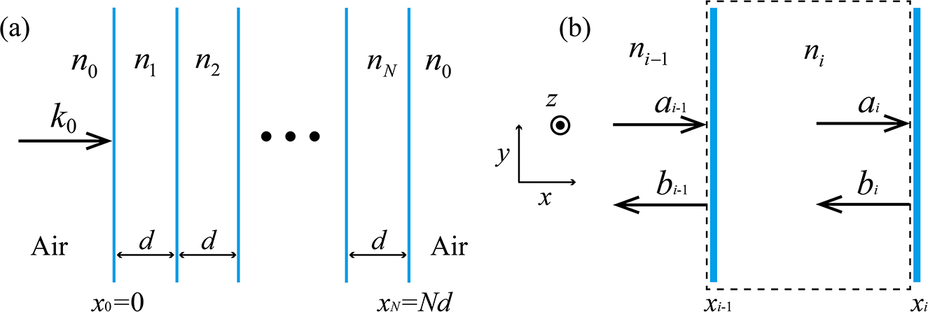
(Color online) (a) The 1D random system composed of random dielectric layers (white) with gain/lossy coatings (blue). The whole system is embedded in air. (b) The schematic of wave propagations inside the 1D random system. The black dashed line indicates the choice of the i-th scattering element. 1D, one dimensional.

In order to study the Anderson localization of the system, we take the following more general form for the relative permittivity of the interface coating between the (i−1)-th and i-th layers:

where α is a dimensionless parameter that controls the strength of gain/loss. It is easy to see from Eq. (1) that the sum of Im(εi−1,i) for all interfaces is zero. Thus, the system as a whole has no net gain or loss. Since the transmission is always unity for normally incident waves when α = 1 independent of random configuration or sample size, the Anderson localization length diverges at this critical point. We will study the divergent behavior of the Anderson localization length when α is close to unity. We will also study the divergent behavior for obliquely incident waves at α = 1 when the incident angle is close to zero.

By utilizing Eq. (1) and the Maxwell’s equations, we can obtain the boundary conditions at an interface, say, x=xi−1 for a harmonic wave with frequency ω (see Supplementary Note 2 for details):

where E_i,y (H_i,y) and E_i,z (H_i,z) are the y and z components of the electric (magnetic) field in the i-th layer, respectively, and Z₀ is the vacuum impedance. Equations (2) and (3) describe the continuity of the tangential components of the electric field. However, the two tangential components of magnetic field are not continuous due to the presence of the imaginary part of the permittivity at the interface, which acts as a current source in the direction parallel/antiparallel to the tangential components of the electric field, as shown in Eqs. (4) and (5). Equations (2)–(5) show that due to the vanishing thickness of the coating layer, the real part of the permittivity of the coating does not play a role in the boundary conditions.

It is important to point out that when α = 1, Eq. (1) always gives unity transmission with zero reflection when the wave with wavevector k₀ in the background medium is incident from the left, independent of the random arrangement [37]. In this case, the magnitude of electric field is a constant in all layers. To see this explicitly, we consider the case when the electric and magnetic fields are aligned with the y and z axes, respectively, i.e., E_y and H_z. Let (Ei−1,y, Hi−1,z) and (Ei,y, Hi,z) be the electric and magnetic fields of the incident wave in the layer i−1 and transmitted wave in the layer i, respectively. If there is no reflection, the boundary conditions in Eqs. (2) and (5) give the following energy flux change across the interface between layer i−1 and i

It is easily seen that the above change of energy flux obeys the Poynting theorem

∇⋅S=−ωIm(ε)⋅|E(x=xi−1)|2 if Im(ε) has the form prescribed in Eq. (1) with α = 1. Thus, the difference in energy flux on each side is totally compensated by the energy flux produced or dissipated at the interface coating and the assumption of no reflection produces the correct physical solution. However, if the wave is incident from the right, the direction of the energy flux is reversed, the energy flux difference changes its sign and reflection will occur in order to make the energy flux conserved.

When α ≠ 1, reflections occur on both sides of an interface, and Anderson localization will occur as a result of coherent backscattering effects. This is also true for oblique incidence even when α = 1.

In order to study the transport properties of the above system, we consider an N-layer sample shown in Figure 1(a) as a successive stack of N + 1 scattering elements. In Figure 1(b), we show the i-th scattering element as the region from the right end of the (i−1)-th layer, x=xi−1, to that of the i-th layer, x=xi. Using the transfer-matrix method (TMM), one can obtain the transmission and reflection amplitudes across each scattering element. For the i-th scattering element, we let ti+(ri+) be the transmission (reflection) amplitude for waves incident from the left (forward waves), and ti−(ri−) for waves incident from the right (backward waves). Then, for forward waves, the transmission amplitude t+(N+1) through the stack of N + 1 scattering elements can be obtained from the following recurrence relations [33], [34], [35], [36] starting from i = 1 till i = N,

where t+(i) and r−(i) denote the forward transmission amplitude and backward reflection amplitude of the first i scattering elements, respectively. Note that when i = 1, we have t+(1)=t1+ and r−(1)=r1−. From Eq. (7), we obtain the transmission coefficient TN=|t+(N+1)|2, and

By applying the recursion equation (9) iteratively, we can express T_N as

Next, we use the TMM to obtain the transmission and reflection amplitudes of an individual scattering element. For normal incidence, as shown in Figure 1(b), the electric fields can be expressed as:

in the (i−1)-th layer, and

in the i-th layer. Here k₀ is the wave vector in vacuum. The magnetic fields can be obtained through the relation Hi=Ei/Zi, where Zi=μ0/εi is the impedance of the i-th layer.

Using the boundary conditions in Eqs. (2)–(5), we can obtain the transfer matrix m⁽ⁱ⁾ connecting the electric fields at the interfaces x = x_i−1 and x = x_i,

with

The transmission and reflection amplitudes of the i-th scattering element can be obtained from the transfer matrix:

It is easily seen that when α = 1 we have m21(i)=0 and m12(i)≠0, leading to zero reflection for wave incident from left and finite reflection for waves coming from right. Since this behavior is true for all layers, we will have unity transmission and zero reflection for waves entering from the left of the sample. Since the system is reciprocal, unity transmission is also expected for waves coming from right side of the sample even though the reflection is not zero.

3 Anomalous Anderson localization behaviors

We first study the Anderson localization behaviors for the case of normal incidence when α deviates slightly from unity. In this case, reflections occur on both sides of every scattering element. As a result, coherent backscattering-induced Anderson localization can occur, similar to the case of Hermitian random media. The localization length ξ can be obtained from the geometrical mean of the transmission coefficient according to the relation:

where L = Nd is the sample length and <>_c denotes ensemble averaging.

In our numerical study, we set k₀ and d to be unity for simplicity. As will see in Section 4 that the critical behaviors will not be altered if these parameters are scaled according to k′d′ = k₀d = 1. We first use Eqs. (13)–(19) to obtain the transmission and reflection amplitudes of each scattering element. Then by applying the recursion equations (7) and (8) iteratively, we obtain the transmission coefficient T_N from Eq. (9). In Figure 2(a) and (b), we plot 〈lnTN〉c as a function of the sample length L = Nd (solid circles) at four different values of α for both the cases of α < 1 and α > 1. Each data point of 〈lnTN〉c shown here (as well as in other figures of this work) is obtained from an average of over 200 configurations and the length L used in the calculation of 〈lnTN〉c is about five times of the localization length. For each value of α, the plot of 〈lnTN〉c vs. L can be well fitted into a straight line with a negative slope, indicating the exponential decay of the transmission T_N with increasing L, i.e., the occurrence of Anderson localization. Following Eq. (20), we can obtain the localization length ξ through the slope of the linear fitting. In the insets of Figure 2(a) and (b), we plot the localization length lnξ as a function of ln|α−1| for the above two cases, respectively. From the linear fits, we get

with A₋ = 4.110, B₋ = −1.007, A₊ = 9.139 and B₊ = −1.010. We can see that for both cases, the log–log plots of ξ vs. |α−1| follow a straight line with a slope −1 as indicated by the blue lines in the insets, which indicates a ξ∝|α−1|−v behavior with the exponent ν = 1. Although the critical exponent of ξ is the same for both α < 1 and α > 1, the magnitude of ξ is about 150 times larger in the region of α > 1 than in the region of α < 1 for a given value of |α−1|. As we will see below, the asymmetry between α > 1 and α < 1 also leads to very different Anderson localization behaviors in the two regions for obliquely incident waves. The origin of such significant asymmetry will be discussed in Section 4.

Figure 2:

(Color online) (a) The ensemble averaged ln T_N as a function of the sample length L for different values of α < 1. (b) Same as (a), but for α > 1. The purple, yellow, blue and green solid circles in (a) denote the numerical results for α = 0.999, 0.998, 0.997 and 0.996, respectively, while in (b) for α = 1.002, 1.004, 1.006 and 1.008. The solid lines are linear fits for different values of α in both (a) and (b). The insets show the localization length ξ retrieved from the slope of the linear fit for different values of |α−1| (solid circles) for both α < 1 [inset in (a)] and α > 1 [inset in (b)] cases. All numerical results in the insets are well fitted by a relation ξ∝|α−1|v with v = 1 for both α < 1 and α > 1.

In the above simulations, the strength of gain/loss is tuned simultaneously by changing the value of α for all interface coatings. We can also consider the case where the value of α in each coating layer is distributed randomly in an interval [1−Δ, 1+Δ]. Our simulation results show that the Anderson localization length follows the ξ∝Δ−1 behavior. Here, the inverse localization length is found to be linearly proportional to the disorder strength Δ of the gain/loss. This is different from the quadratic behavior normally found in random Hermitian systems [3]. The detailed results are shown in Supplementary Note 3.

Now, we study the Anderson localization behaviors when waves are obliquely incident with an incident angle θ₀. We consider S-polarized waves, where the electric field E is perpendicular to the plane of incidence. In this case, the electric field behaves as a scalar wave and can be expressed as (see Figure 3)

in the (i−1)-th layer, and

in the i-th layer. Using the boundary conditions Eqs. (2)–(5) and the impedance relation H=ε/μ0⋅E, we obtain the following transfer matrix m⁽ⁱ⁾ connecting the electric fields at the interfaces x_i−1 and x_i:

where sinθi=n0sinθ0/ni and θ₀ is the incident angle. It is easy to see that Eqs. (25)–(28) reduce to Eqs. (14)–(17) when θ₀ = 0. By substituting Eqs. (25)–(28) into Eqs. (18) and (19) and using Eqs. (7)–(9), we can study the dependence of 〈lnTN〉c on the sample length L. It is expected that the localization length diverges when θ₀ = 0 and α = 1. The results of α = k₀ = 1 are shown in Figure 4 for different incident angles (solid circles). It can be seen that 〈lnTN〉c decays linearly with the sample length L for all incident angles, indicating Anderson localization. In the inset of Figure 4, we plot the localization length ξ (retrieved from the linear fitting of 〈lnTN〉c vs. L) as a function of incident angle. We find that the log-log plot of ξ vs. sinθ0 shows a straight line, indicating a ξ∝sin−v′θ0 behavior at small θ₀. To obtain the critical exponent v′, we use the following linear equation,

Figure 3:

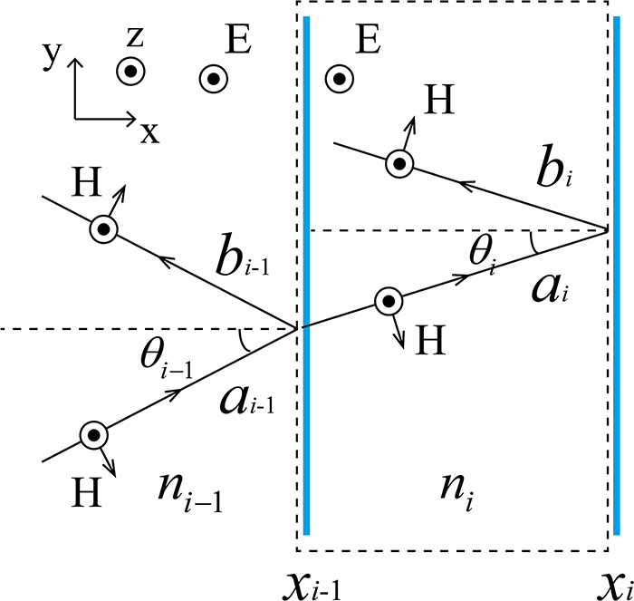
(Color online) The schematic of wave propagations for S-polarized waves.

Figure 4:

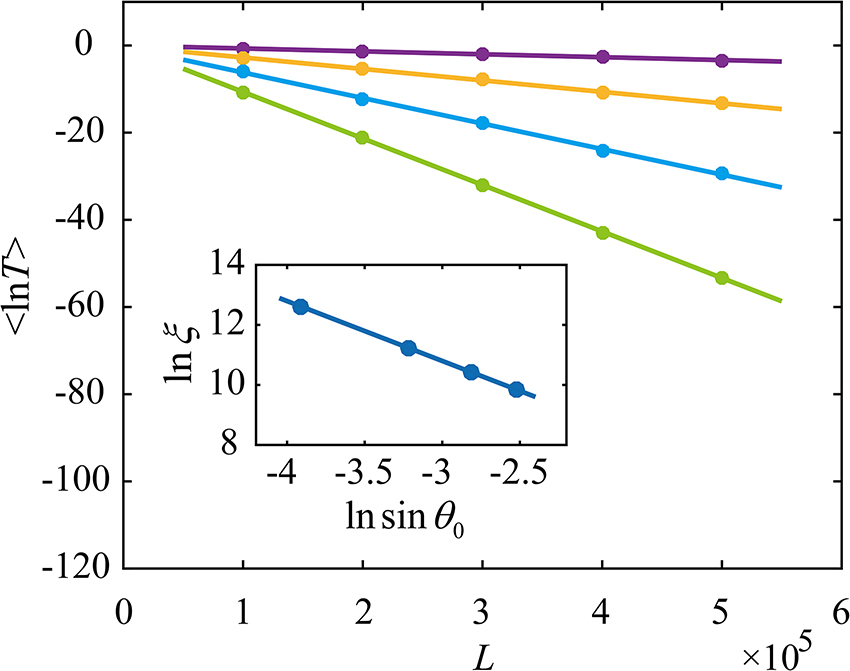
(Color online) The ensemble averaged lnT_N as a function of the sample length L for different incident angles for S-polarized waves when α = 1. The purple, yellow, blue and green solid circles denote the numerical results for sin θ₀ = 0.02, 0.04, 0.06 and 0.08, respectively. The solid lines are linear fittings. The inset shows the localization length ξ retrieved from the slope of the linear fitting for different sinθ0 (solid circles), which are well fitted by a relation ξ∝sin−2θ0(solid line).

to fit the numerical results and obtain A_S = 4.810 and B_S = −1.996. The value of the slope suggests an exponent v′=2, i.e., ξ∝sin−2θ0. This result is distinctly different from those found in Hermitian impedance-matched 1D random systems [31] and pseudospin-1 system [32], in which the exponents found are both v′=4 rather than v′=2.

As the model of uniformly distributed random dielectric constants studied above is difficult to realize, we have also studied the Anderson localization behavior of a binary random system, which consists of two kinds of dielectric layers with relative permittivity either 0.5 or 1.5 with equal probability. Our simulation results show the same critical behavior ξ∝sin−2θ0 as that of the uniformly distributed random media, in line with the concept of universality. The detailed results are given in Supplementary Note 4.

In the following, we study the Anderson localization behaviors when α deviates from unity. In Figure 5, we plot the numerical results of the inverse localization length 1/ξ as a function of α for different incident angles. These results suggest the following simple expression for the inverse localization length in the region of α ≤ 1:

where A and B are two constants. If we use the fitting results of Eqs. (21) and (29) to set the values of A and B, i.e., A=exp(−A−)=1.640×10−2 and B=exp(−AS)=8.146×10−3, Eq. (30) gives excellent fitting results of the data at three incident angles in the region of α ≤ 1 as shown by the solid lines in Figure 5. Eq. (30) indicates that the localization length at any point (1−α, θ0) in the critical region is simply the harmonic mean of the localization length at point (1−α, θ0=0) and the localization length at point (α=1, θ0). This also suggests that 1−α and θ₀ are two independent parameters in the determination of Anderson localization in the critical region of α ≤ 1. However, the localization behavior in the region of α > 1 is more complicated. As shown in Figure 5, for all the incident angles studied sinθ0≠0, the function 1/ξ first follows the linear decay of Eq. (30) to a minimum value and then turn around and increases linearly with α. The existence of a linear term 1−α instead of a quadratic term in Eq. (30) explains the asymmetry in the magnitudes of the localization length in the regions of α < 1 and α > 1 shown in Figure 2.

Figure 5:

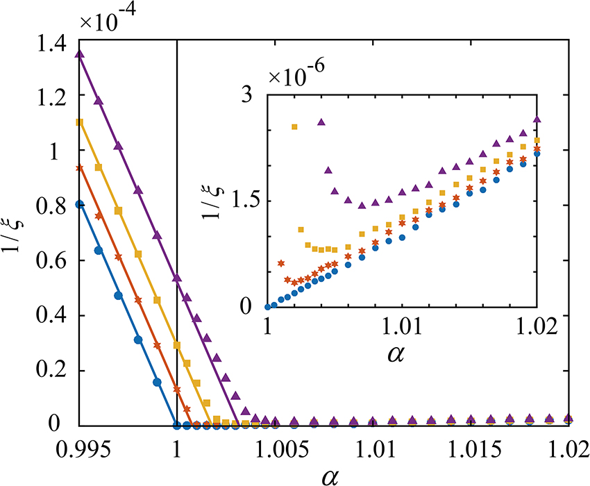
(Color online) The plot of inverse localization length 1/ξ as a function of α at different incident angles. The blue circles, red hexagrams, yellow squares and purple triangles denote numerical results for sin θ₀ = 0, 0.04, 0.06 and 0.08, respectively. The straight lines are the results of Eq. (30). The α = 1 is marked by a black solid line. The inset shows the details at small values of 1/ξ in the region of α ≥ 1.

4 The origin of anomalous Anderson localization behaviors

In this section, we will start from the stack recursion equation (10) to understand the above anomalous localization behaviors. As can be seen from Eq. (10), the log of the transmission consists of two terms: the first term ∑i=1N+1ln|ti+|2 involves the transmission coefficients of individual scattering elements only, and we call it noninterference term; the second term −2∑i=2N+1ln|1−ri+r−(i−1)| involves both the modulus and phase of the reflection amplitudes and we will refer to it as the interference term. The stack recursion equation method has been discussed in detail in the literature [33], [34], [35], [36].

We first consider the case of normal incidence. In the critical region, we can write α = 1 + δ with δ being a small positive or negative number. By substituting Eqs. (14)–(17) into Eqs. (18) and (19) and taking the small δ limit, we obtain the following expressions for the transmission and reflection amplitudes of the i-th scattering element:

It should be noted that k₀ appears only in the phase factors of Eqs. (31)–(34) and scales with 1/d, In our simulations, we have chosen k₀ = d = 1. The choice of another k′0 will not change the total transmission T_N in Eq. (10) if the layer thickness is scaled to d′=k0d/k′0. According to Eq. (20), such scaling will only change the localization length of the system by a factor d′/d. It will not change its critical behavior. To the lowest order in δ, the noninterference term in Eq. (10) can be expressed as

Thus, the ensemble average of the noninterference term can be written as

The above linear dependence in δ actually gives rise to both the unity critical exponent and the localization length asymmetry between the regions of δ > 0 and δ < 0. For the uniform distribution of the relative permittivity in the interval [1−σ, 1+σ], the coefficient C₁ (σ) can be evaluated as

For our case σ = 0.5, we can get C₁ (σ = 0.5) = 0.0239. It is important to point out that the linear dependence of the noninterference term shown in Eq. (36) acts as a delocalization effect when δ > 0 as it enhances the transmission. Similarly, using Eq. (33), we can expand the ensemble average of the interference term in Eq. (10) as

where the subscripts ‘+’ and ‘−’ in C2,±(1)(σ, k0d) denote the coefficients calculated in the regions of α > 1 and α < 1, respectively. The difference is due to the term r−(i−1) in Eq. (38), which has different behaviors across the critical point at α = 1. From Eqs. (10), (20), (36) and (38), the localization length can be expressed as ξ≅−2dC1(σ)+limN→∞C2,±(1)(σ, k0d)δ−1 for the normal incidence, which shows explicitly the ξ∝|α−1|−1 behavior found in Figure 2. Since we have already obtained numerically the divergent behavior of ξ in Eqs. (21) and (22) for the case of k₀ = d = 1, i.e., ξ±≅exp(A±)⋅δ−1, the values of limN→∞C2,±(1)(0.5, 1) can be obtained from the values of A± and C₁ (σ = 0.5), from which we can get limN→∞C2,−(1)(σ=0.5, 1)=0.00887 and limN→∞C2,+(1)(σ=0.5, 1)=−0.0241. Note that C2,−(1)(0.5, 1) and C2,+(1)(0.5, 1) have the opposite signs so that C2,±(1)(0.5, 1)⋅δ is always negative, which means the interference term always gives positive contribution to the localization effect. From the above analysis, it is clearly seen that the unity critical exponent arising from the linear term δ in the expansion of ln T_N of Eq. (10) is independent of the choices of k₀d and σ. And the significant asymmetry found in the localization lengths between the regions α < 1 and α > 1 is due to the delocalization effect of the noninterference term in the region α > 1, which significantly enlarge the localization length.

Now we consider the case of oblique incidence with α = 1. To obtain the transmission and reflection amplitudes of the i-th scattering element at small θ₀, we expand Eqs. (25)–(28) to the leading order in θ₀ and obtain

where ρ=n0sinθ0. Using Eq. (40), the noninterference term can be written as

The ensemble average of the noninterference term can be expressed as

where

Then we can get D₁ (σ = 0.5) = −0.0134 by substituting σ = 0.5.

Using Eq. (39), the ensemble average of interference term can be expressed as:

where D2(1) denotes the coefficient of the leading term in small ρ². We can now express the localization length as ξ=−2dD1(σ)+limN→∞D2(1)(σ, k0d)ρ−2, which shows exactly the ξ∝sin−2θ0 behavior found in Figure 4. From the result of ξ≅exp(AS)⋅δ−1 in Eq. (29) and the value of D₁ (σ) in Eq. (45), we found limN→∞D2(1)(σ=0.5, k0d=1)=−0.00289. From Eqs. (36), (38), (44) and (46), it is clearly seen that the critical exponents ν and ν′ do not dependent on the choice of σ. Thus, our results are universal for different strengths of randomness.

5 Conclusion

We have numerically studied the Andersion localization behavior of the incident waves of a given wavevector k₀ in 1D random layered non-Hermitian media with sample-specific gain and loss inserted between any two adjacent layers as described in Eq. (1). At normal incidence θ₀ = 0, the systems always possess unity transmission at a specific strength of gain and loss (α = 1 in Eq. (1)), independent of the random configuration and the sample size. The existence of such an infinite localization length allows us to study the behavior of Anderson localization in a small critical region surrounding the critical point. We found the following anomalous behaviors. In the case of normal incidence, the localization length behaves like ξ≈A|α−1|−1. While the exponent ν is the same in both regions of α > 1 and α < 1, the prefactor A in the region of α > 1 is much greater than that in the α < 1 region. In the case of oblique incidence (θ₀ ≠ 0), the localization length behaves like ξ≈Bsin−2θ0 for S-polarized waves at α = 1. The exponent ν′=2 is different from the behavior ξ∝1/sin4θ0 found in impedance-matched systems and pseudospin-1 Hermitian systems. We have also studied the localization length behavior at oblique incidence when α ≠ 1. Very different behaviors are found between the region of α > 1 and α < 1 even though the system is gain/loss balanced on average in both cases. The asymmetry of the localization behaviors in the two regions is due to the presence of a delocalization effect in the noninterference term when α > 1, which makes the localization length very large compared to that in the α < 1 region.

We note that in ordinary Hermitian random media, the critical point is normally at the ordered media where the localization length diverges. The addition of sample-specific balanced gain and loss in 1D media can move the critical point from ordered to disordered media. This allows us to study the Anderson localization behavior of non-Hermitian disordered systems in the vicinity of its critical point. Although our study was done for some specific choices of disorder strength σ = 0.5, the critical exponents found here are universal and independent of the choices of σ as can be seen in Section 4. We have also studied a few cases of k₀d ≠ 1 and found that different values of k₀d will only change the magnitude of the localization length. The exponents ν = 1 and ν′=2 remain unchanged.

References

[1] P. W. Anderson, “Absence of diffusion in certain random lattices,” Phys. Rev., vol. 109, no. 5, p. 1492, 1958, https://doi.org/10.1103/physrev.109.1492.Search in Google Scholar
[2] A. Lagendijk, B. Van Tiggelen, and D. S. Wiersma, “Fifty years of Anderson localization,” Phys. Today, vol. 62, no. 8, pp. 24–29, 2009, https://doi.org/10.1063/1.3206091.Search in Google Scholar
[3] P. Sheng, Scattering and localization of classical waves in random media, World Scientific, 1990.10.1142/0565Search in Google Scholar
[4] D. S. Wiersma, P. Bartolini, A. Lagendijk, and R. Righini, “Localization of light in a disordered medium,” Nature, vol. 390, no. 6661, pp. 671–673, 1997, https://doi.org/10.1038/37757.Search in Google Scholar
[5] M. Störzer, P. Gross, C. M. Aegerter, and G. Maret, “Observation of the critical regime near Anderson localization of light,” Phys. Rev. Lett., vol. 96, no. 6, 2006, Art no. 063904, https://doi.org/10.1103/physrevlett.96.063904.Search in Google Scholar
[6] T. Schwartz, G. Bartal, S. Fishman, and M. Segev, “Transport and Anderson localization in disordered two-dimensional photonic lattices,” Nature, vol. 446, no. 7131, pp. 52–55, 2007, https://doi.org/10.1038/nature05623.Search in Google Scholar PubMed
[7] P. Sheng and Z. Q. Zhang, “Scalar-wave localization in a two-component composite,” Phys. Rev. Lett., vol. 57, no. 15, p. 1879, 1986, https://doi.org/10.1103/physrevlett.57.1879.Search in Google Scholar PubMed
[8] S. John, H. Sompolinsky, and M. J. Stephen, “Localization in a disordered elastic medium near two dimensions,” Phys. Rev. B, vol. 27, no. 9, p. 5592, 1983, https://doi.org/10.1103/physrevb.27.5592.Search in Google Scholar
[9] M. Y. Azbel, “Eigenstates and properties of random systems in one dimension at zero temperature,” Phys. Rev. B, vol. 28, no. 8, p. 4106, 1983, https://doi.org/10.1103/physrevb.28.4106.Search in Google Scholar
[10] V. Baluni and J. Willemsen, “Transmission of acoustic waves in a random layered medium,” Phys. Rev., vol. 31, no. 5, p. 3358, 1985, https://doi.org/10.1103/physreva.31.3358.Search in Google Scholar PubMed
[11] C. M. de Sterke and R. C. McPhedran, “Bragg remnants in stratified random media,” Phys. Rev. B, vol. 47, no. 13, p. 7780, 1993.10.1103/PhysRevB.47.7780Search in Google Scholar PubMed
[12] F. M. Izrailev, A. A. Krokhin, and N. M. Makarov, “Anomalous localization in low-dimensional systems with correlated disorder,” Phys. Rep., vol. 512, no. 3, pp. 125–254, 2012, https://doi.org/10.1016/j.physrep.2011.11.002.Search in Google Scholar
[13] C. Miniatura, L. C. Kwek, M. Ducloy, et al., Eds. Ultracold Gases and Quantum Information: Lecture Notes of the Les Houches Summer School in Singapore, vol. 91, July 2009, Oxford University Press; 2011, Chap. 9.10.1093/acprof:oso/9780199603657.001.0001Search in Google Scholar
[14] A. Yamilov and B. Payne, “Classification of regimes of wave transport in quasi-one-dimensional non-conservative random media,” J. Mod. Optic., vol. 57, no. 19, pp. 1916–1921, 2010, https://doi.org/10.1080/09500340.2010.519443.Search in Google Scholar
[15] A. A. Asatryan, N. A. Nicorovici, L. C. Botten, C. M. de Sterke, P. A. Robinson, and R. C. McPhedran, “Electromagnetic localization in dispersive stratified media with random loss and gain,” Phys. Rev. B, vol. 57, no. 21, p. 13535, 1998, https://doi.org/10.1103/physrevb.57.13535.Search in Google Scholar
[16] A. Yamilov, S. H. Chang, A. Burin, A. Taflove, and H. Cao, “Field and intensity correlations in amplifying random media,” Phys. Rev. B, vol. 71, no. 9, 2005, Art no. 092201, https://doi.org/10.1103/physrevb.71.092201.Search in Google Scholar
[17] J. Heinrichs, “Light amplification and absorption in a random medium,” Phys. Rev. B, vol. 56, no. 14, p. 8674, 1997, https://doi.org/10.1103/physrevb.56.8674.Search in Google Scholar
[18] V. Freilikher, M. Pustilnik, and I. Yurkevich, “Effect of absorption on the wave transport in the strong localization regime,” Phys. Rev. Lett., vol. 73, no. 6, p. 810, 1994, https://doi.org/10.1103/physrevlett.73.810.Search in Google Scholar PubMed
[19] Z. Q. Zhang, “Light amplification and localization in randomly layered media with gain,” Phys. Rev. B, vol. 52, no. 11, p. 7960, 1995, https://doi.org/10.1103/physrevb.52.7960.Search in Google Scholar PubMed
[20] S. Kalish, Z. Lin, and T. Kottos, “Light transport in random media with PT symmetry,” Phys. Rev., vol. 85, no. 5, 2012, Art no. 055802, https://doi.org/10.1103/physreva.85.055802.Search in Google Scholar
[21] T. S. Misirpashaev, J. C. J. Paasschens, and C. W. J. Beenakker, “Localization in a disordered multi-mode waveguide with absorption or amplification,” Phys. Stat. Mech. Appl., vol. 236, no. 3-4, pp. 189–201, 1997, https://doi.org/10.1016/s0378-4371(96)00387-1.Search in Google Scholar
[22] S. A. Ramakrishna, E. K. Das, G. V. Vijayagovindan, and N. Kumar, “Reflection of light from a random amplifying medium with disorder in the complex refractive index: statistics of fluctuations,” Phys. Rev. B, vol. 62, no. 1, p. 256, 2000, https://doi.org/10.1103/physrevb.62.256.Search in Google Scholar
[23] X. Jiang, Q. Li, and C. M. Soukoulis, “Symmetry between absorption and amplification in disordered media,” Phys. Rev. B, vol. 59, no. 14, 1999, Art no. R9007, https://doi.org/10.1103/physrevb.59.r9007.Search in Google Scholar
[24] P. K. Datta, “Transmission and reflection in a perfectly amplifying and absorbing medium,” Phys. Rev. B, vol. 59, no. 16, 1999, Art no. 10980, https://doi.org/10.1103/physrevb.59.10980.Search in Google Scholar
[25] R. Frank, A. Lubatsch, and J. Kroha, “Theory of strong localization effects of light in disordered loss or gain media,” Phys. Rev. B, vol. 73, no. 24, 2006, Art no. 245107, https://doi.org/10.1103/physrevb.73.245107.Search in Google Scholar
[26] L. Y. Zhao, C. S. Tian, Z. Q. Zhang, and X. D. Zhang, “Unconventional diffusion of light in strongly localized open absorbing media,” Phys. Rev. B, vol. 88, no. 15, 2013, Art no. 155104, https://doi.org/10.1103/physrevb.88.155104.Search in Google Scholar
[27] H. Cao, Y. G. Zhao, S. T. Ho, E. W. Seelig, Q. H. Wang, and R. P. H. Chang, “Random laser action in semiconductor powder,” Phys. Rev. Lett., vol. 82, no. 11, p. 2278, 1999, https://doi.org/10.1103/physrevlett.82.2278.Search in Google Scholar
[28] H. Cao, J. Y. Xu, D. Z. Zhang, et al., “Spatial confinement of laser light in active random media,” Phys. Rev. Lett., vol. 84, no. 24, p. 5584, 2000, https://doi.org/10.1103/physrevlett.84.5584.Search in Google Scholar
[29] A. A. Chabanov, M. Stoytchev, and A. Z. Genack, “Statistical signatures of photon localization,” Nature, vol. 404, no. 6780, pp. 850–853, 2000, https://doi.org/10.1038/35009055.Search in Google Scholar PubMed
[30] V. Milner and A. Z. Genack, “Photon localization laser: low-threshold lasing in a random amplifying layered medium via wave localization,” Phys. Rev. Lett., vol. 94, no. 7, 2005, Art no. 073901, https://doi.org/10.1103/physrevlett.94.073901.Search in Google Scholar PubMed
[31] K. Kim, “Anderson localization of electromagnetic waves in randomly-stratified magnetodielectric media with uniform impedance,” Optic Express, vol. 23, no. 11, pp. 14520–14531, 2015, https://doi.org/10.1364/oe.23.014520.Search in Google Scholar
[32] A. Fang, Z. Q. Zhang, S. G. Louie, et al., “Anomalous Anderson localization behaviors in disordered pseudospin systems,” Proc. Natl. Acad. Sci. Unit. States Am., vol. 114, no. 16, pp. 4087–4092, 2017, https://doi.org/10.1073/pnas.1620313114.Search in Google Scholar PubMed PubMed Central
[33] A. Fang, Z. Q. Zhang, S. G. Louie, and C. T. Chan, “Nonuniversal critical behavior in disordered pseudospin-1 systems,” Phys. Rev. B, vol. 99, no. 1, 2019, Art no. 014209, https://doi.org/10.1103/physrevb.99.014209.Search in Google Scholar
[34] M. Born and E. Wolf, Principles of optics, 7th ed. Cambridge, Cambridge University Press, 2002.Search in Google Scholar
[35] A. A. Asatryan, L. C. Botten, M. A. Byrne, et al., “Suppression of Anderson localization in disordered metamaterials,” Phys. Rev. Lett., vol. 99, no. 19, p. 193902, 2007, https://doi.org/10.1103/physrevlett.99.193902.Search in Google Scholar PubMed
[36] M. V. Berry and S. Klein, “Transparent mirrors: rays, waves and localization,” Eur. J. Phys., vol. 18, no. 3, p. 222, 1997, https://doi.org/10.1088/0143-0807/18/3/017.Search in Google Scholar
[37] K. G. Makris, A. Brandstötter, P. Ambichl, Z. H. Musslimani, and S. Rotter, “Wave propagation through disordered media without backscattering and intensity variations,” Light Sci. Appl., vol. 6, no. 9, 2017, Art no. e17035, https://doi.org/10.1038/lsa.2017.35.Search in Google Scholar PubMed PubMed Central
[38] E. Rivet, A. Brandstötter, K. G. Makris, H. Lissek, S. Rotter, and R. Fleury, “Constant-pressure sound waves in non-Hermitian disordered media,” Nat. Phys., vol. 14, no. 9, pp. 942–947, 2018, https://doi.org/10.1038/s41567-018-0188-7.Search in Google Scholar
[39] C. M. Bender and S. Boettcher, “Real spectra in non-Hermitian Hamiltonians having P T symmetry,” Phys. Rev. Lett., vol. 80, no. 24, p. 5243, 1998, https://doi.org/10.1103/physrevlett.80.5243.Search in Google Scholar
[40] C. M. Bender, D. C. Brody, and H. F. Jones, “Complex extension of quantum mechanics,” Phys. Rev. Lett., vol. 89, no. 27, 2002, Art no. 270401, https://doi.org/10.1103/physrevlett.89.270401.Search in Google Scholar
[41] S. Longhi, “Optical realization of relativistic non-Hermitian quantum mechanics,” Phys. Rev. Lett., vol. 105, no. 1, 2010, Art no. 013903, https://doi.org/10.1103/physrevlett.105.013903.Search in Google Scholar
[42] S. Longhi, “PT-symmetric laser absorber,” Phys. Rev., vol. 82, no. 3, 2010, Art no. 031801, https://doi.org/10.1103/physreva.82.031801.Search in Google Scholar
[43] Y. D. Chong, L. Ge, and A. D. Stone, “P t-symmetry breaking and laser-absorber modes in optical scattering systems,” Phys. Rev. Lett., vol. 106, no. 9, 2011, Art no. 093902, https://doi.org/10.1103/physrevlett.106.093902.Search in Google Scholar
[44] J. Luo, J. Li, and Y. Lai, “Electromagnetic impurity-immunity induced by parity-time symmetry,” Phys. Rev. X, vol. 8, no. 3, 2018, Art no. 031035, https://doi.org/10.1103/physrevx.8.031035.Search in Google Scholar
[45] L. Ge, Y. D. Chong, and A. D. Stone, “Conservation relations and anisotropic transmission resonances in one-dimensional PT-symmetric photonic heterostructures,” Phys. Rev., vol. 85, no. 2, 2012, Art no. 023802, https://doi.org/10.1103/physreva.85.023802.Search in Google Scholar
[46] R. Fleury, D. L. Sounas, and A. Alu, “Negative refraction and planar focusing based on parity-time symmetric metasurfaces,” Phys. Rev. Lett., vol. 113, 2014, Art no. 023903, https://doi.org/10.1103/physrevlett.113.023903.Search in Google Scholar
Supplementary material
The online version of this article offers supplementary material (https://doi.org/10.1515/nanoph-2020-0306).
© 2020 Tianshu Jiang et al., published by De Gruyter, Berlin/Boston
This work is licensed under the Creative Commons Attribution 4.0 International License.
Articles in the same Issue
- Editorial
- Optoelectronics and Integrated Photonics
- Disorder effects in nitride semiconductors: impact on fundamental and device properties
- Ultralow threshold blue quantum dot lasers: what’s the true recipe for success?
- Waiting for Act 2: what lies beyond organic light-emitting diode (OLED) displays for organic electronics?
- Waveguide combiners for mixed reality headsets: a nanophotonics design perspective
- On-chip broadband nonreciprocal light storage
- High-Q nanophotonics: sculpting wavefronts with slow light
- Thermoelectric graphene photodetectors with sub-nanosecond response times at terahertz frequencies
- High-performance integrated graphene electro-optic modulator at cryogenic temperature
- Asymmetric photoelectric effect: Auger-assisted hot hole photocurrents in transition metal dichalcogenides
- Seeing the light in energy use
- Lasers, Active optical devices and Spectroscopy
- A high-repetition rate attosecond light source for time-resolved coincidence spectroscopy
- Fast laser speckle suppression with an intracavity diffuser
- Active optics with silk
- Nanolaser arrays: toward application-driven dense integration
- Two-dimensional spectroscopy on a THz quantum cascade structure
- Homogeneous quantum cascade lasers operating as terahertz frequency combs over their entire operational regime
- Toward new frontiers for terahertz quantum cascade laser frequency combs
- Soliton dynamics of ring quantum cascade lasers with injected signal
- Fiber Optics and Optical Communications
- Propagation stability in optical fibers: role of path memory and angular momentum
- Perspective on using multiple orbital-angular-momentum beams for enhanced capacity in free-space optical communication links
- Biomedical Photonics
- A fiber optic–nanophotonic approach to the detection of antibodies and viral particles of COVID-19
- Plasmonic control of drug release efficiency in agarose gel loaded with gold nanoparticle assemblies
- Metasurfaces for biomedical applications: imaging and sensing from a nanophotonics perspective
- Hyperbolic dispersion metasurfaces for molecular biosensing
- Fundamentals of Optics
- A Tutorial on the Classical Theories of Electromagnetic Scattering and Diffraction
- Reflectionless excitation of arbitrary photonic structures: a general theory
- Optimization Methods
- Multiobjective and categorical global optimization of photonic structures based on ResNet generative neural networks
- Machine learning–assisted global optimization of photonic devices
- Artificial neural networks for inverse design of resonant nanophotonic components with oscillatory loss landscapes
- Adjoint-optimized nanoscale light extractor for nitrogen-vacancy centers in diamond
- Topological Photonics
- Non-Hermitian and topological photonics: optics at an exceptional point
- Topological photonics: Where do we go from here?
- Topological nanophotonics for photoluminescence control