Application of laser scanning technology for structure gauge measurement
-
Michal Strach
 and
Przemyslaw Grabias
and
Przemyslaw Grabias

Abstract
One of the basic conditions guaranteeing safe and collision-free operation of rail vehicles is maintaining the structure gauge. Verification of the location of rail infrastructure components is carried out using various measurement techniques. This article describes the accuracy of the gauge measurement with the use of a scanning tachymeter. Tachymetric measurements and laser scanning technology were used in the experimental study of the tram loop area. The analysis covered the possibility of using a point cloud to determine geometrical relationships among the track, traction poles and the overhead line. The quality of the laser scanning data in terms of the measurement frequency, the laser beam angle of incidence per object and the average reflection intensity was examined. Performed verification was based on the data from tachymetric measurements. In the tested area, the track consists of straight sections and several circular arcs of small radii and variable curvature. The specific geometry of the track required calculation of the gauge extension parameters depending on the curve radius. In addition, a horizontal track alignment design was prepared. The designed location of the track and extended dimensions of the structure gauge were used to verify the correct spatial position of the current track in relation to the infrastructure elements.
1 Introduction
Recent years have seen a significant development in laser scanning technology and popularisation of its applications in surveying. This technique is typically used as an alternative, a complementary or, in some cases, a substitute for classic measurements. Its potential can be exploited in the inventory surveys of transport corridors such as roads and rail routes. Due to its high measurement efficiency, mobile laser scanning is the most common technology that can be complemented by terrestrial laser scanning. LIDAR data are utilised for inventory surveys of rail transport objects. The advantage of laser scanning over conventional measurement techniques is the flexibility of the data for further development. Classical measurement is usually performed for one specific task. It is often done with the use of different measuring instruments. Conversely, the laser scanner provides the material for a variety of analyses. A point cloud with the appropriate density and accuracy allows for the comprehensive analysis of track geometry, structure gauge and overhead contact line. In the study of geometric relationships between many elements of the same object, it is advisable to use a measurement technique that provides a full range of data.
The most popular of the conducted studies include testing geometry and maintenance of tunnels [1,2], automatic detection of track geometry [3,4], automatic recognition of track components [5] and track centres [6,7,8] as well as structure gauge measurement [9,10]. Data obtained with various measuring sensors such as vision systems based on video cameras and thermal imaging cameras constitute a valuable complement to point clouds originating from laser scanning. Data from these systems can be employed, among others, for the analysis of structure gauge [11], the location of track faults [12,13], the wear analysis of the overhead power traction cables [14,15] and the location of short circuits [16].
Scanning tachymeters are devices combining the features of electronic tachymeters, terrestrial laser scanners and instruments for terrestrial photogrammetry. These devices are based on motorised, reflectorless electronic tachymeters with high accuracy of angle and distance measurements. One of the basic elements of the scanning tachymeter equipment is a camera integrated with the device’s angle measurement system. It provides a visualisation of the field work area and the detailed photographic documentation of the measurements. Scanning tachymeters are used in applications where it is sufficient to perform quick measurements of small and medium objects with a detailed supplementation of scans and photographs of fragments of elements of complex geometry. The low scanning speed of scanning tachymeters compared to that of laser scanners should be taken into account in the process of deciding whether to use this technology. Scanning tachymeters can be used for inventorying and determining geometric imperfections of coating structures, examining the shape and deformation of structures, determining the volume of bulk material heaps, monitoring geotechnical structures and inventorying historic buildings for the purpose of their renovation and maintenance [17,18].
The structure gauge is an important issue encountered in rail transport, including railways, subways and trams. It is defined as a clear space determined by a line defining minimum distances between a rail vehicle and components of rail transport infrastructure [19,20]. This space is necessary to ensure safe and collision-free operation of rail vehicles. Currently, most studies focus on the measurement of the railway gauge. Techniques most often utilised include mobile scanning systems equipped with additional sensors and mounted on locomotives, railway wagons, draisines and track measuring trolley [21,22]. Mobile measurements can be complemented by terrestrial laser scanning, which is applied at sites where a mobile scanner was not able to conduct object measurements (due to object covering or niches) or where higher accuracy of measurement is expected. The use of terrestrial laser scanning may also have economic justification in the case of inventory surveys of small and geometrically complex objects. These may include a bridge, tunnel, switch or a tram loop. Tracks located at a loop are characterised by complex geometry. Moreover, a dense network of electric traction elements is situated along their length. The basic research carried out at a tramway loop involves the examination of the structure gauge and the track geometry.
This article describes tests of the Leica Nova MS50 scanning tachymeter conducted at a tram loop in Krakow. Data obtained from the scanner were compared with tachymetric measurements. High accuracy of the scan results allowed comprehensive analyses to be performed at the examined site. Complexity of the procedure applied for gauge maintenance verification was also demonstrated. Consequently, the horizontal track alignment design was prepared, and gauge extension parameters – calculated and additionally, spatial placement of contact wires in relation to the track – were verified. Moreover, the study necessitated conducting an analysis of the current regulations for tramway design [23,24,25] and inventory surveys [26,27].
2 Experimental object and method of conducting measurements
The experimental study was conducted at the “Wieczysta” tram loop in Krakow built in 1964 and thoroughly modernised in 2015. The object comprises three electrified track segments of total length 490 m and four turnouts. Detailed measurements focused on the 290 m long exterior track loop, along which 16 traction poles are situated. The chosen track consists of straight segments and circular arcs of varying curvature (arcs’ radii ranging from 22 to 50 m). The measurement was carried out with the use of the Leica Nova MS50 scanning tachymeter that demonstrates the following accuracy parameters: angle measurement, ±0.5″; single prism measurement, ±0.6 mm + 1 mm/km; reflectorless measurement, ±2 mm + 2 mm/km [28]. The equipment is versatile due to its high precision and the speed of operation maintained in both the motorised tachymeter and the laser scanner mode. Laser scanning and tachymetric reflectorless measurements were conducted for the track and all catenary poles including contact wire clamps.
High-quality point clouds have been obtained by using a precise scanning tachymeter. On the basis of these point clouds, it was possible to locate individual elements of the infrastructure with the accuracy of single millimetres. The applied measurement technology guarantees a wide spectrum of analyses, including track geometry, structure gauge and contact wire position in relation to the track axis.
The accuracy of the laser scanning technique was verified based on the reference data obtained via tachymetric measurement. The analyses were carried out for four catenary poles, namely, p12, p13, p14 and p15 (Figure 1a) chosen for their specific location. They are situated consecutively, but each of them is placed on a track segment demonstrating different geometric properties. The examined track section is located on a circular arc with a radius of 21.970 m, then of 50.000 m, next a straight segment along a tram turnout and then an arc with a radius of 22.050 m. Changing circular arc radii affects the analysis of the gauge maintenance. This issue will be described later in this article.
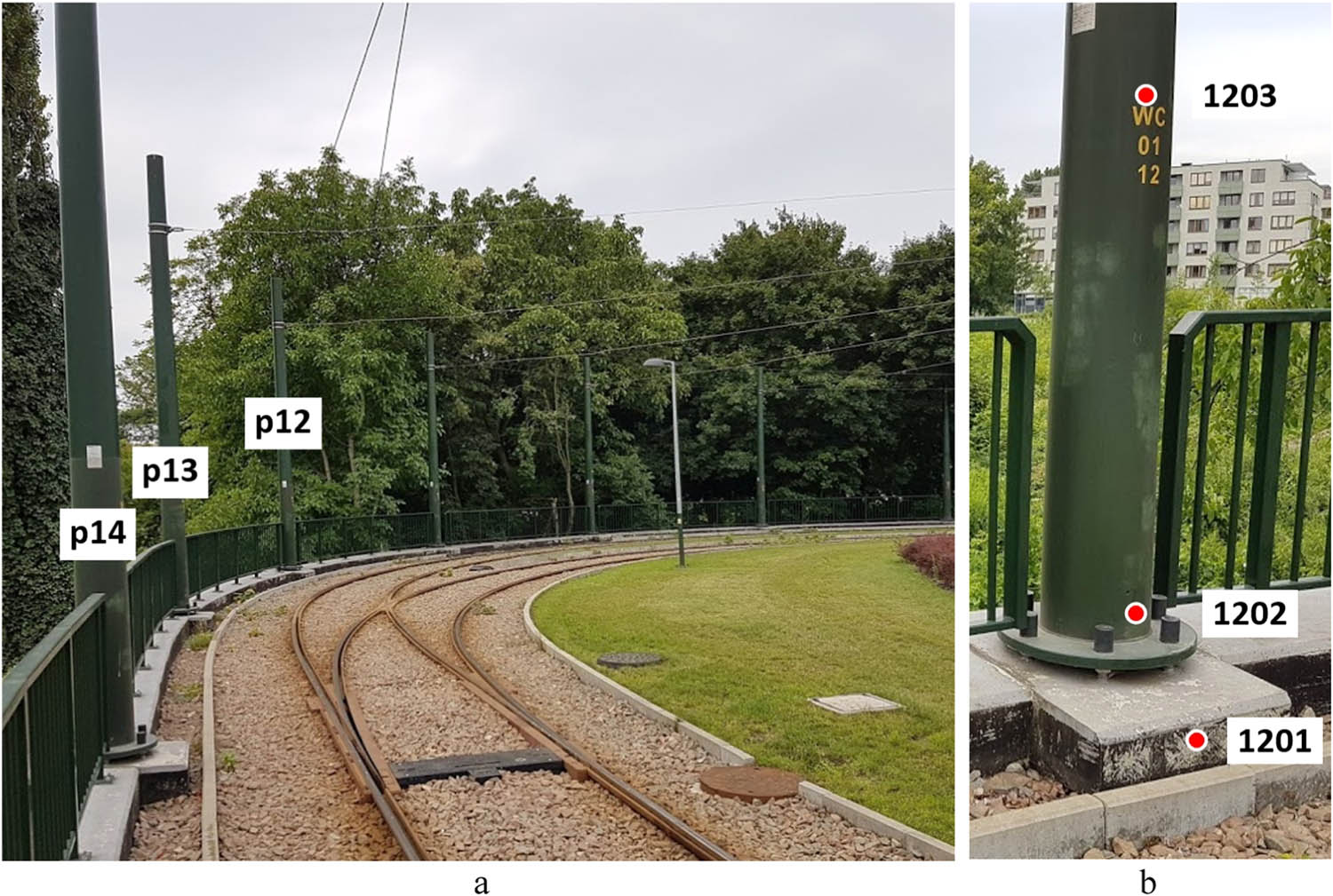
View of the tram loop section with numbered catenary poles (a) and points on the p12 mast showing the tachymetric measurement locations (b).
Four points were measured on each of the four selected poles (Figures 1b and 2a). The choice of the measured points was influenced by the classical approach to the measurement of structure gauge on railway lines. As a standard, it is a point located on the foundation of the catenary pole, as well as three points, namely, at the base of the catenary pole, on the fixed point and below the mounting bracket that supports the contact wires. Intended analyses required certain preparation of the measurement data obtained with the scanning tachymeter. A reference to the congruent geodetic control points was made at each measurement station, which enabled individual point clouds to be oriented into one spatial coordinate system. Their merge resulted in a common cloud of points representing spatial imaging of objects located at the tramway loop, among others, the tram track and poles as well as elements of overhead electric traction.
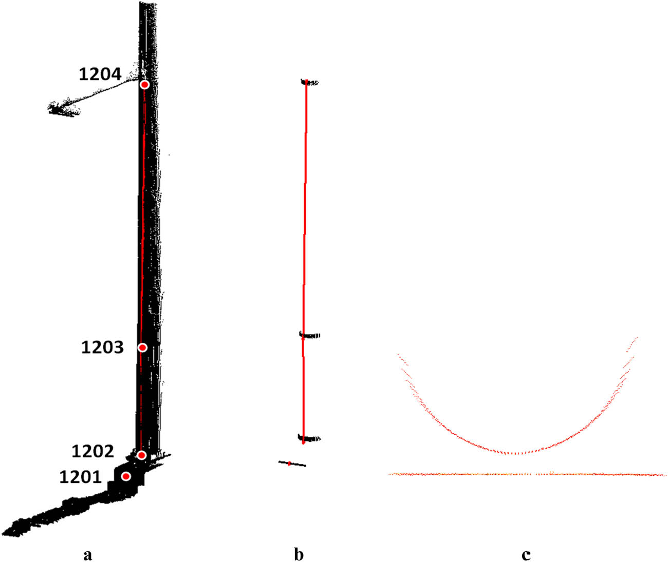
A fragment of the point cloud representing a catenary pole and a track (a), cloud sections in the vicinity of points measured tachymetrically (b) and cloud cross-sections into which a straight segment and a circle (c) were fitted.
Moreover, the impact of the scanning mode (resolution parameter) on the accuracy of the results was also examined. In the case of poles no. p12, p13 and p14, the scan was performed with the frequency of 62 pts/s and the resolution of 10 mm at a distance of 10 m. However, a higher operating frequency was adopted for the pole p15, which consequently resulted in reducing the scanning time by half.
3 Testing terrestrial laser scanning accuracy
The analysed point cloud was reduced to cross-sections covering a catenary pole, elements of the overhead contact line network and the track sector located opposite to the pole (Figure 2a). Four fragments situated near the points obtained via the tachymetric measurement (Figure 1b.) were selected at each of the cross-sections (Figure 2b). Cloud fragments representing catenary poles take a shape resembling a semicircle, while the distribution of points on the pole’s foundation takes a shape resembling a straight line (Figure 2c).
Obtained sections contain points with known spatial coordinates, which made it possible to fit a straight line or a circle into the individual sets of points using the regression method. Depending on the type of the fitted element, the coordinates of the circle’s centre and radius or of the straight line’s beginning and end were determined. It is also possible to model 3D traction poles, but in this case, it is not necessary. In the structure gauge analysis, only the horizontal distance of the traction pole dropped perpendicularly on the track axis is relevant. To simplify the calculations, a fragment of a point cloud located around the analysed point was dropped on a horizontal plane.
The accuracy analysis of the elements’ positioning in relation to the points measured tachymetrically was carried out separately for the circle and the straight line. It involved calculating the distance between the fitted element and the point obtained from the tachymetric measurement. In the case of an arc, it was radial, while the analysis of orthogonal method’s measurements was applied for straight lines. Obtained differences are summarised in Table 1, which also includes information for each of the points regarding the vertical measurement angle, the measurement frequency and the average intensity of the laser beam reflection from the measured surface. The vertical measurement angle is the angle between the horizon and the direction towards particular points (Figure 3a). In the analysed case, at vertical angles close to 0, the laser beam incidence angle was perpendicular to the given scanned catenary pole.
Fitting results and measurement characteristics conducted with a scanning tachymeter
| Catenary pole no. | Point no. | Fitted element type | Distance [mm] | Vertical angle [°] | Measurement frequency [Hz] | Average reflection intensity |
|---|---|---|---|---|---|---|
| p12 | 1,201 | Straight line | 0.4 | −14 | 62 | 1,978 |
| 1,202 | Circle | 0.8 | −11 | 2,012 | ||
| 1,203 | 0.4 | 2 | ||||
| 1,204 | 2.0 | 33 | ||||
| p13 | 1,301 | Straight line | 0.3 | −10 | 62 | 1,983 |
| 1,302 | Circle | 1.3 | −8 | 2,014 | ||
| 1,303 | 0.7 | 2 | ||||
| 1,304 | 2.8 | 26 | ||||
| p14 | 1,401 | Straight line | 0.6 | −10 | 62 | 1,971 |
| 1,402 | Circle | 1.2 | −8 | 2,010 | ||
| 1,403 | 2.1 | 2 | ||||
| 1,404 | 2.5 | 23 | ||||
| p15 | 1,501 | Straight line | 1.4 | −10 | 250 | 1,979 |
| 1,502 | Circle | 1.8 | −7 | 2,015 | ||
| 1,503 | 1.1 | 3 | ||||
| 1,504 | 2.7 | 26 |
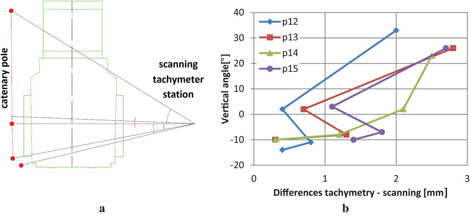
The relationship between the laser beam’s angle of incidence (a) and the obtained differences of laser scanning and tachymetric measurement results (b).
Several conclusions can be drawn from the results of the point cloud fitting. The increase in the horizontal angle value increases the value of differences between the element fitted from the point cloud and the actual surface of the object measured tachymetrically. The biggest differences can be observed for points ranging from 0.0020 to 0.0027 m located highest on the poles (Figure 3b). Selected points are located, among others, at the minimum and maximum height of the catenary pole. The measurements to these points are characterized by extreme angles of the laser beam. For these points, the largest measurement errors were recorded. There is no justification for increasing the number of points on the pole for purposes of accuracy analysis. Errors for points located at other heights will be smaller than errors for extreme points.
According to the Leica Nova MS50 technical specification [28], when scanning at a frequency of 62 Hz for measuring distances up to 50 m, the range noise is 0.6 mm. Similarly, while scanning at a frequency of 250 Hz with the same measuring distance, the range noise is 0.8 mm. The absolute position accuracy of a modelled surface is similar to a reflectorless single measurement, which is 2 mm + 2 ppm (according to the ISO standards). The survey results confirm this value. The results summarised in Table 1 show that there are no significant differences in accuracy between measurements taken at two different frequencies.
The shape adopted by the object’s surface translates into the type of the fitted element affecting the accuracy of the test results. The discrepancy for straight lines fitted into flat surface ranged from 0.0003 to 0.0014 m, while the discrepancy achieved for circles doubled, ranging from 0.0004 to 0.0027 m. The average reflection intensity is higher in the case of metal covered with a dark green paint than in the case of concrete protected with a black polymer compound. There are studies [29,30] presenting the analysis of the influence on the type of the measured surface, its colour and the material of which it is made. They also take into account the changes in the angle of incidence of the laser beam on the surface and the influence of its refraction. These studies confirm the conclusions of the article.
The accuracy of the laser scanning survey conducted with the use of the Leica Nova MS50 robotic tachymeter was confronted with the requirements concerning tram line measurements and diagnostics. They do not directly specify the criteria regarding the accuracy of the gauge measurement, but define permissible deformations and determine a tolerance of 0.025 m [20] for the lateral track displacement. Therefore, more restrictive requirements included in the railway guidelines were adopted for the purpose of the gauge analysis. A permissible difference of a track position in relation to the adjacent track and infrastructure facilities (including traction poles) cannot exceed ±0.020 m [26]. However, there are no guidelines for measuring the gauge accuracy on tram lines.
Performance of all analyses shows that, regardless of the angle of incidence of the laser beam, the measurement accuracy required by the applicable regulations is maintained. The technique examined is sufficiently accurate for the selection of optimal field measurement procedures. In the analysed case, the measurement was performed with a precise instrument with target values not exceeding 30 m. It allows the determination of the 3D point location at the level of individual millimetres. The obtained point cloud was characterized by high density, and the measured surface had good reflective properties. Attempts were also made to avoid sharp angles of the laser beam falling on the inventoried surface.
4 Verification of the maintenance of the gauge
A tram structure gauge is an outline of a plane figure providing the basis to determine the clearance necessary for efficient tram traffic, which would exclude all structures, installations and objects located at the track except the contact wire. Tram trackways should be designed in such a way as to maintain sufficient distances between the structure gauge and the kinematic gauge, along which the rolling stock moves, to ensure traffic safety [19,25,26].
As far as tram tracks are concerned, the structure gauge can be divided into the continuous (Figure 4a) and point structure gauge (Figure 4b). The former refers to an object whose dimension measured along the tram tack exceeds 3 m, and the latter refers to an object smaller or equal to 3 m. The necessary clearance outline is the underdeveloped space whose cross-section constitutes a polygon of such dimensions and shape, which enables a tram truck to travel within its borders with the velocity ranging from zero to a maximum authorised speed [20].
![Figure 4 Tram gauge of continuous (a) and point structures (b) for 1,435 mm-wide track [20].](/document/doi/10.1515/geo-2020-0056/asset/graphic/j_geo-2020-0056_fig_004.jpg)
Tram gauge of continuous (a) and point structures (b) for 1,435 mm-wide track [20].
Measurement data obtained with the laser scanning technique provided the basis for the analysis of the structure gauge maintenance at the tram loop, which is an interesting object demonstrating characteristics different from standard tram routes. Tram transport follows specific guidelines, which allow for specific cases of values and some parameter tolerance cited later in this article. Due to the fact that the only objects encountered at the tram loop are catenary poles, only point structure gauge analysis can be conducted.
It is worth mentioning that the positioning of the tram rolling stock at curvilinear track sections differs from that at straight sections. To preserve traffic safety, the clearance outline at horizontal and vertical track curvatures is increased about a set value with respect to the standard gauge dimensions. The clearance extensions enable trams to pass the curvatures safely even if inclining beyond the standard outline, which is especially relevant within curves of a small radius.
There are several extension parameters, each of them adjusts the gauge dimensions to a different aspect of spatial tram positioning and their values are dependent on the track curve radius. P value indicates the structure gauge broadening at the track curve at the carriage level. It takes different dimensions for the interior (concave) and the exterior (convex) sides of the curvature. Q parameter refers to the extension at the wheel and pantograph level, while parameter V determines lowering of the bottom edge of the gauge at a vertical arc. The values have been calculated according to the following formulas [20]:
where Pi is the half-width outline extension of the necessary underdeveloped space on the concave side of the curve (m) and R is the horizontal curve radius (m).
where Pa is the half-width outline extension of the necessary underdeveloped space on the convex side of the arc (m) and R is the horizontal curve radius (m).
Symbol
where Q is the half-width outline extension of the necessary underdeveloped space at the level of the wheels and pantograph at the concave side of the curve (m) and R is the horizontal curve radius (m).
where V is lowering of the structure gauge bottom edge at a concave arc (m) and Rv is the horizontal curve radius (m).
The execution of the regulation project and determining the basic parameters of track axis geometry are not directly related to the analysis of the quality of laser scan data. However, it is an essential link in the process of analysing geometric relationships between the elements of technical infrastructure. Data determining the 3D position of the track axis and information on the radius length of individual circular arcs were necessary to carry out a comprehensive verification of the structure gauge and the analysis of the position of electric traction wires.
Calculating the gauge outline extension parameters correctly requires knowledge of the curves’ radii available, among others, in a construction project. In the analysed case, the length of the horizontal curve radius was 22 and 50 m. Unfortunately, the project lacked data concerning the beginnings and ending (kilometrage) of the individual geometric elements. The possibility of track deformation due to operational stress was also taken into consideration. In the case of rail routes, it manifests in the form of track element degradation and spatial shifts of track centres. Track displacements may affect structure gauge maintenance, and in general, the safety of tramway transport. Geodetic measurements provide data necessary to determine current track geometry and its deviation from the design assumptions. In the analysed case, the tachymetric measurement of the track was carried out opposite to all catenary poles and at cross-sections spaced every 5 m at rectilinear sections and every 2 m on curvilinear ones. The coordinates of the tram track centres were the basis for the preparation of the horizontal track alignment design. The goal of the project was to determine geometrical parameters of the examined track and adjustments necessary to restore its optimal shape. Track alignment design was executed in a specialised application (Bentley Rail Track) based on the multiple horizontal element regression analysis using least-squares solver, that is, the Gauss–Jordan method. The following factors were taken into consideration: minimizing horizontal displacements, maintaining similar to the design geometrical parameters of the curvilinear sections, preserving track spacing and proper structure gauge. The studies provided comprehensive data regarding the track geometry and track lateral displacements at the measured cross-sections. Table 2 lists the horizontal curve radii dimensions opposite to which the traction poles are located. All of them approximate the values cited in the loop documentation. The maximum differences in the radii length are as follows: −0.030 m (pole p12) and +0.053 m (pole p15). Designed radii were utilised to calculate potential gauge extension. The individual parameters are presented in Table 2. In addition, drawings presenting the outline of the standard and the extended gauge (Figure 5a) as well as the visualisation of the results were also prepared. Each of the gauge outlines was fitted into the cross-section through a point cloud opposite to the catenary poles (Figure 5b).
Gauge extension parameters for individual catenary poles
| Pole no. | R [m] | Gauge extension [m] | |||
|---|---|---|---|---|---|
| Concave side of a curve (Pi) | Convex side of a curve (Pa) | Wheels and pantograph level (Q) | Bottom edge lowering (V) | ||
| p12 | 21.970 | 0.228 | 0.127 | 0.023 | 0.000 |
| p13 | 50.000 | 0.100 | 0.007 | 0.010 | 0.000 |
| p14 | Straight line | 0.000 | 0.000 | 0.000 | 0.000 |
| p15 | 22.053 | 0.227 | 0.124 | 0.023 | 0.000 |

Current gauge (red colour) and the extended gauge (green colour) on the arc (a) and the view of the fitted cross-sections of the gauge (b).
Apart from graphical verification of the gauge maintenance, numerical analyses were also prepared. First, they focused on the examination of the distances between the catenary poles and the tram track centre. The distances between the track axis and the pole foundation (point 1,201) at 1.5 m above the track gradeline were calculated for each of the poles (point 1,203), and the results are plotted at the cross-section drawings (Figure 6). The figure also includes dimensions of clear space located between the pole and the extended gauge outline. Table 3 presents detailed computation results of the distance between point structures, the track centre and the structure gauge outline.
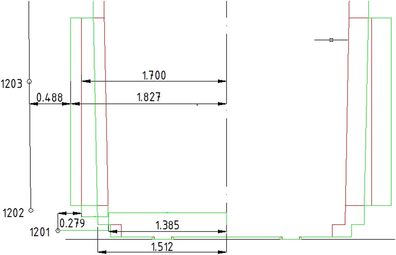
Analysis of the point structure gauge maintenance for the pole p12.
Results of the point structure gauge analysis
| Point no. | Obstacle – track centre distance [m] | Min. distance maintaining the gauge [m] | Clear space – old track centre [m] | Track centre displacement [m] | Clear space – new track centre [m] |
|---|---|---|---|---|---|
| 1,201 | 1.908 | 1.512 | 0.396 | 0.000 | 0.396 |
| 1,301 | 1.931 | 1.392 | 0.539 | 0.002 | 0.537 |
| 1,401 | 1.883 | 1.385 | 0.498 | 0.018 | 0.480 |
| 1,501 | 1.930 | 1.509 | 0.421 | −0.027 | 0.448 |
| 1,203 | 2.262 | 1.827 | 0.435 | 0.000 | 0.435 |
| 1,303 | 2.290 | 1.707 | 0.583 | 0.002 | 0.581 |
| 1,403 | 2.247 | 1.700 | 0.547 | 0.018 | 0.529 |
| 1,503 | 2.288 | 1.824 | 0.464 | −0.027 | 0.491 |
Another important element of the analysis was verification of the gauge maintenance after taking into consideration the corrections of the track position postulated by the prepared track alignment design. Transversal track displacements opposite to the catenary poles range from +0.018 to −0.027 m. Table 3 presents the values of the offsets and the adjusted clearance.
The minimal value of clear space refers to the catenary pole foundation p12 and is equal to 0.396 m. While the maximal distance for the point on the pole p13 is 0.583 m. It is worth mentioning that the smallest safe distances for both types of points was recorded for the mast p12, where the track’s radius is the shortest and the gauge’s radius is the broadest. An average distance of clear space for the analysed points is 0.485 m. The calculations were supplemented with a graphical representation of the gauge location for cross-sections situated opposite to catenary poles, which is depicted in Figure 7. Geometrical relationships between the old and new track centres as well as the gauge and the masts are shown in the form of a horizontal projection. The results from Figure 7 and Table 3 support the conclusions that the structural gauge is preserved at the examined section and fulfils the assumed requirements with a sufficient safety margin.

Graphical representation of the gauge location for the cross-sections situated opposite to catenary poles.
5 Overhead network analysis
Trams are powered by electricity provided via overhead network that consists of cables, running rails and wires supplying electricity to rolling stock and discharging it to a substation [23]. The overhead contact line comprises a set of wires suspended over the track providing power directly to a tram and includes contact wires held by messenger wires and droppers as well as catenary wires supported by line structures and masts placed every few meters.
Contact wires are held in place by brackets and come into direct contact with a pantograph. Consequently, they are subjected to natural wear over time. To minimise the wear of the slipping component of the current collector, the contact wire is zigzagged. It involves applying the offset, with the use of extraction arms, alternately to the left and right in relation to the track centre. The zigzag allows the pantograph elements to wear evenly, thus extending their service life. Pursuant to the standard [23], regular tramway network offset should be ±0.30 m on a straight line and ±0.35 m on an arc. The maximum allowable offset is ±0.40 m.
Comprehensive studies of spatial positioning of the railway infrastructure elements should also include contact wires. Data regarding geometrical relations between the track axis and the contact wire are crucial. Elements of the overhead contact line, along with the contact wire, were surveyed in one measurement together with the catenary poles for gauge analysis. This shows the various possibilities of the technique used in relation to related issues within one object.
The analysis began with determining the zigzagging placement of the wire. The verification was carried out for points located in the centre of each of the 16 retaining clips situated opposite to the traction poles numbered from p7 to p22. First, the spatial location of the overhead line clip and messenger wire fixing point was determined on the point cloud. An example of a point cloud presenting traction elements is shown in Figure 8.
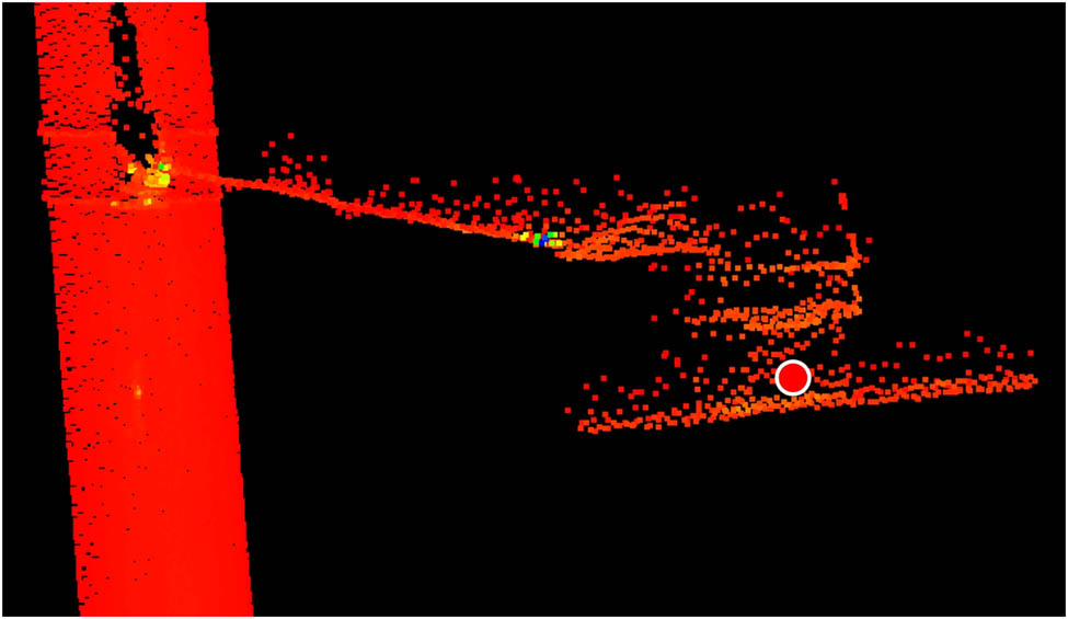
View of the scanned overhead line retaining clip with the messenger wire fixing point marked.
The obtained points were connected with a polyline representing the actual overhead line placement. The offset of the contact wire at a given point was defined as a horizontal shift between the polyline and the track centre. The axis placement was computed in the horizontal track alignment design on the basis of the tachymetric measurements. Comprehensive data regarding spatial positioning of the overhead line and track centre made it possible to calculate the distance in sections every 1 m. The zigzag graph for the 16 retaining clips and the position of the contact wire in relation to the track axis are presented in Figure 9, where a black, thickened line with the value of 0.000 m indicates the track centre, and red dotted ones indicate a maximal allowable offset. In the case of most analysed points, the tolerance for the offset was preserved, while for a few of them, the recommended value was slightly exceeded.
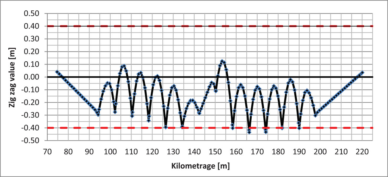
Diagram of the contact wire offset at 1 m intervals.
The analysis of laser scanning accuracy was carried out for the traction poles. When scanning overhead contact line cables, it was assumed that the accuracy will be comparable and not worse than the accuracy given in the technical specification of the device. The maximal contact wire shift in relation to the track centre is 0.435 m for the pole p17. Consequently, the highest deviation from the maximum allowable offset was 0.035 m. As anticipated, the maximal values were recorded at the retaining clips, and the minimal ones were recorded at halfway between successive traction poles. The geometry of the track as well as the location of traction poles has an impact on exceeding the permissible offset. In the analysed case, their placement was defined already at the design stage, and the density results from a very limited space available at the tram loop. According to the current regulations, the recommended distance between adjacent clips on the arc with a 22 m radius is 7.90 m [23]. In the analysed case, it ranged between 7.80 and 8.25 m (Figure 10). Exceeding the recommended distances between traction poles explains the resulting violation of the allowable offset for the overhead line.
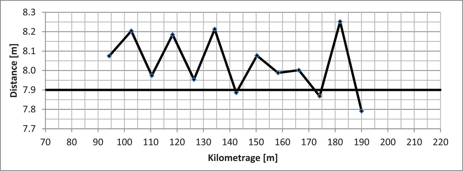
Distances between contact wire retaining clips.
Determination of the contact wire suspension height in relation to the top of rail was another issue analysed in this study. A comprehensive set of data, equivalent to the one used for determining the horizontal offset, was applied. In this case, however, the focus was on the values in the vertical plane, which were calculated as differences between the height of retaining clips, obtained with the laser scanner and the height of the track centre, recorded via a tachymetric measurement. The nominal contact wire suspension height is measured from the level of the rail head and, according to the regulations, is normally set to 5.50 m [23]. In the case of a tram loop, it is possible to reduce this height to 5.0 m. In contrast, the maximum cable suspension height is 5.70 m. Permissible deviations of the given values are +0.10 and −0.25 m. The contact wire height in relation to the level of the running surface took values from 5.48 to 5.67 m (Figure 11). All of them fall within the acceptable range from 5.00 to 5.70 m applicable to a tram loop. The average height of the cable suspension for the analysed section is 5.63 m. The smallest values were recorded at the cross-sections opposite to the extreme outer traction poles (p7 and p22).
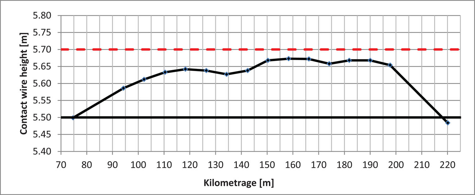
Diagram of the contact wire suspension height.
6 Conclusions
Inventory surveys of buildings and technical infrastructure can be conducted with commonly used classic measurement techniques. However, more and more often they are replaced by terrestrial and mobile laser scanning. The growing popularity of this modern measuring technology is due to its many advantages, since it offers noncontact, fast, detailed (high resolution) and precise measurement of objects. The tests have demonstrated high versatility of the Leica Nova MS50 scanning tachymeter. The device enables quick and precise measurement to be made to the geodetic control network, which provides both the tachymetric single point and the point cloud measurements with orientation in a fixed spatial coordinate system. The tested device, depending on the needs and the accuracy requirements, could be used both as a scanner and a tachymeter. The inventory of objects at the tram loop is carried out with varying accuracy. Measurements with accuracy of a few millimetres are conducted for the purpose of tram track alignment. In this case, it is best to use a tachymetric measurement at intervals of a few dozen meters along the track centre. Slightly lower requirements regard measuring the structure gauge. The location of traction poles, power cables and distances between adjacent tracks should be determined with an accuracy ranging from a few to up to a dozen or so millimetres. Laser scanning can be utilised for such purposes.
However, it should be remembered that the time needed to acquire a point cloud depends on the size of the area being scanned as well as the frequency and the density of the scan. Taking the aforementioned factors into consideration, such work optimisation should be considered that would limit the scope of scanning only to sections containing selected infrastructure objects. With lower accuracy requirements for determining the spatial position of objects, the measurement frequency can be increased, while the density of the measurement can be reduced. Changing the scanning parameters significantly shortens the measurement time at a given point. Modification of the scan parameters, especially the distance to the scanned items, also affects the measurement accuracy. In the case of a tram loop, the scanned objects were located at distances not exceeding 30 m. Consequently, only a slight decrease in the accuracy of the measurement could be observed. The results fell within acceptable limits.
Laser scanning technology provided accurate and versatile data concerning spatial positioning of the objects at the tram loop. The structure gauge analysis at curvilinear track sections requires technical expertise necessary for calculating the geometrical parameter of track centre and structure gauge extensions and determining optimal track alignment corrections. The effects of working on the point cloud despite being satisfactory are time consuming, which is due to the partial or complete lack of tools that automate data processing. The preparation of computational algorithms and proper selection of software would automate and accelerate the process of analysing and developing results.
Acknowledgments
The article was prepared under the research subvention of AGH University of Science and Technology No. 16.16.150.545 in 2019.
References
[1] Weixing W, Weisen Z, Lingxiao H, Vivian V, Zhiwei W. Applications of terrestrial laser scanning for tunnels: a review, J Traffic Transport Eng (Engl Ed). 2014;1(5):325–37.10.1016/S2095-7564(15)30279-8Search in Google Scholar
[2] Strach M, Dronszczyk P. Comprehensive 3D measurements of tram tracks in the tunnel using the combination of laser scanning technology and traditional TPS/GPS surveying. Transport Res Proc. 2016;14:1940–9. 10.1016/j.trpro.2016.05.161.Search in Google Scholar
[3] Leslar M, Perry G, McNease K. Using mobile Lidar to survey a railway line for asset inventory. In: Proceedings of the American Society for Photogrammetry and Remote Sensing (ASPRS) Annual Conference, San Diego, CA, USA, 26–30 April, 2010, pp. 1–8.Search in Google Scholar
[4] Gabara G, Sawicki P. A new approach for inspection of selected geometric parameters of a railway track using image-based point clouds. Sensors. 2018;18(3):791. 10.3390/s18030791.Search in Google Scholar PubMed PubMed Central
[5] Pastucha E. Catenary system detection, localization and classification using mobile scanning data. Remote Sens. 2016;8(10):801. 10.3390/rs8100801.Search in Google Scholar
[6] Elberink SO, Moustafa A, Khoshelham K, Diaz-Benito D. Rail track detection and modelling in mobile laser scanner data, ISPRS. Ann Photogramm Remote Sens Spatial Inf Sci. 2013;II(5/W2):223–8. 10.5194/isprsannals-II-5-W2-223-2013.Search in Google Scholar
[7] Elberink SO, Khoshelham K. Automatic extraction of railroad centerlines from mobile laser scanning data. Remote Sens. 2015;7(5);5565–5583. 10.3390/rs70505565.Search in Google Scholar
[8] Kregar K, Možina J, Ambrožič T, Kogoj D, Marjetič A, Štebe G et al. Control measurements of crane rails performed by terrestrial laser scanning. Sensors. 2017;17(7):1671. 10.3390/s17071671.Search in Google Scholar PubMed PubMed Central
[9] Mikrut S, Kohut P, Pyka K, Tokarczyk R, Barszcz T, Uhl T. Mobile laser scanning systems for measuring the clearance gauge of railways: state of play, testing and outlook. Sensors. 2016;16(5):683. 10.3390/s16050683.Search in Google Scholar PubMed PubMed Central
[10] Höfler H, Baulig C, Blug A, Wölfelschneider H, Fleischhauer O, Wirth H, et al. High speed clearance profiling with integrated sensors. 7th World Congress on Railway Research, WCRR, Montreal 4–8 June 2006, 282.Search in Google Scholar
[11] Zhan D, Yu L, Xiao J, Chen T. Multi-camera and structured-light vision system (MSVS) for dynamic high-accuracy 3D measurements of railway tunnels. Sensors. 2015;15(4):8664–84. 10.3390/s150408664.Search in Google Scholar PubMed PubMed Central
[12] Ye J, Stewart E, Roberts C. Use of a 3D model to improve the performance of laser-based railway track inspection. Proc Inst Mech Eng Part F J Rail Rapid Transit. 2019;233(3):337–55. 10.1177/0954409718795714.Search in Google Scholar
[13] Deutschl E, Gasser C, Niel A, Werschonig J. Defect detection on rail surfaces by a vision based System. IEEE Intelligent Vehicles Symposium, 2004, pp. 507–11.10.1109/IVS.2004.1336435Search in Google Scholar
[14] Jarzebowicz, L, Judek, S. 3D machine vision system for inspection of contact strips in railway vehicle current collectors. International Conference on Applied Electronics, Pilsen, 2014, pp. 139–144. 10.1109/AE.2014.7011686.Search in Google Scholar
[15] Fukai, H, Watabe, Y, Niwakawa, M, Tabayashi, S. Automatic correction of measurement position Rusing rob ust matching in contact wire inspection system, 11th France-Japan & 9th Europe-Asia Congress on Mechatronics (MECATRONICS)/17th International Conference on Research and Education in Mechatronics (REM), Compiegne, 2016, pp. 193–196. 10.1109/MECATRONICS.2016.7547140.Search in Google Scholar
[16] Dronszczyk, P., Strach, M. The use of laser scanning technology and infrared thermography to survey a tunnel and its fire protection devices (Zastosowanie technologii skaningu laserowego i termowizji do inwentaryzacji tunelu i znajdujących się w nim urządzeń przeciwpożarowych). BiTP. 2016;43(3):199–214. 10.12845/bitp.43.3.2016.18.Search in Google Scholar
[17] Mechelke, K, Kersten, TP, Lindstaedt M. Comparative investigations into the accuracy behaviour of the new generation of terrestrial laser scanning systems. Optical 3-D Measurement Techniques VIII, Gruen/Kahmen (Eds.), Zurich, 2007, July 9–12, Vol. I, pp. 319–327.Search in Google Scholar
[18] Tos, C, Wolski, B, Zielina, L. Application of the scanning total station in geodetic practice (Zastosowanie tachimetru skanującego w praktyce geodezyjnej). Tech Trans Environ Eng. 2010;107(1-S):83–99.Search in Google Scholar
[19] PN-EN 15273-3 + A1:2017-03. Railways – Gauges – Part 3: Structure gauge (Kolejnictwo - Skrajnie - Część 3: Skrajnie budowli).Search in Google Scholar
[20] PN-K-92009: 1998. Public transport – Structure gauge – Requirements. (Komunikacja miejska - Skrajnia budowli – Wymagania).Search in Google Scholar
[21] Engstrand, A. Railway Surveying – A Case Study of the GRP 5000. Master’s Thesis, KTH Royal Institute of Technology, Stockholm, Sweden, 2011.Search in Google Scholar
[22] Chen, Q, Niu, X, Zuo, L, Zhang, T, Xiao, F, Liu, Y, et al. A railway track geometry measuring trolley system based on aided INS. Sensors. 2018;18(2):538. 10.3390/s18020538.Search in Google Scholar PubMed PubMed Central
[23] PN-K-91002:1997. Public transport – Tram and trolleybus overhead line – Requirements. (Komunikacja miejska – Sieć jezdna tramwajowa i trolejbusowa – Wymagania).Search in Google Scholar
[24] PN-K-92011:1998. Tram trackways – Requirements and tests. (Torowiska tramwajowe – Wymagania i Badania).Search in Google Scholar
[25] Technical guidelines for the design, construction and maintenance of tram tracks (Wytyczne techniczne projektowania, budowy i utrzymania torów tramwajowych), MAGTiOŚ, Warsaw, 1983.Search in Google Scholar
[26] Technical standard GK-1 “On the organization and measurement of railway surveying” (Standard techniczny GK-1 “O organizacji i wykonywaniu pomiarów w geodezji kolejowej”), Warsaw, 2015.Search in Google Scholar
[27] Doskocz A. The current state of the creation and modernization of national geodetic and cartographic resources in Poland. Open Geosci. 2016;8(1):579–92. 10.1515/geo-2016-0059.Search in Google Scholar
[28] User Manual for Leica MS50/TS50/TM50, Leica Geosystems AG, Heerbrugg, Switzerland, 2013.Search in Google Scholar
[29] Boehler W, Bordas Vincent M, Marbs A. Investigating laser scanner accuracy. Proceedings of XIXth CIPA Symposium, 2003.Search in Google Scholar
[30] Voegtle T, Schwab I, Landes T. Influences of different materials on the measurements of terrestrial laser scanner (TLS). Proc. of the XXI Congress, the International Society for Photogrammetry and Remote Sensing, ISPRS, 2008.Search in Google Scholar
© 2020 Michal Strach and Przemyslaw Grabias, published by De Gruyter
This work is licensed under the Creative Commons Attribution 4.0 International License.
Articles in the same Issue
- Regular Articles
- The simulation approach to the interpretation of archival aerial photographs
- The application of137Cs and210Pbexmethods in soil erosion research of Titel loess plateau, Vojvodina, Northern Serbia
- Provenance and tectonic significance of the Zhongwunongshan Group from the Zhongwunongshan Structural Belt in China: insights from zircon geochronology
- Analysis, Assessment and Early Warning of Mudflow Disasters along the Shigatse Section of the China–Nepal Highway
- Sedimentary succession and recognition marks of lacustrine gravel beach-bars, a case study from the Qinghai Lake, China
- Predicting small water courses’ physico-chemical status from watershed characteristics with two multivariate statistical methods
- An Overview of the Carbonatites from the Indian Subcontinent
- A new statistical approach to the geochemical systematics of Italian alkaline igneous rocks
- The significance of karst areas in European national parks and geoparks
- Geochronology, trace elements and Hf isotopic geochemistry of zircons from Swat orthogneisses, Northern Pakistan
- Regional-scale drought monitor using synthesized index based on remote sensing in northeast China
- Application of combined electrical resistivity tomography and seismic reflection method to explore hidden active faults in Pingwu, Sichuan, China
- Impact of interpolation techniques on the accuracy of large-scale digital elevation model
- Natural and human-induced factors controlling the phreatic groundwater geochemistry of the Longgang River basin, South China
- Land use/land cover assessment as related to soil and irrigation water salinity over an oasis in arid environment
- Effect of tillage, slope, and rainfall on soil surface microtopography quantified by geostatistical and fractal indices during sheet erosion
- Validation of the number of tie vectors in post-processing using the method of frequency in a centric cube
- An integrated petrophysical-based wedge modeling and thin bed AVO analysis for improved reservoir characterization of Zhujiang Formation, Huizhou sub-basin, China: A case study
- A grain size auto-classification of Baikouquan Formation, Mahu Depression, Junggar Basin, China
- Dynamics of mid-channel bars in the Middle Vistula River in response to ferry crossing abutment construction
- Estimation of permeability and saturation based on imaginary component of complex resistivity spectra: A laboratory study
- Distribution characteristics of typical geological relics in the Western Sichuan Plateau
- Inconsistency distribution patterns of different remote sensing land-cover data from the perspective of ecological zoning
- A new methodological approach (QEMSCAN®) in the mineralogical study of Polish loess: Guidelines for further research
- Displacement and deformation study of engineering structures with the use of modern laser technologies
- Virtual resolution enhancement: A new enhancement tool for seismic data
- Aeromagnetic mapping of fault architecture along Lagos–Ore axis, southwestern Nigeria
- Deformation and failure mechanism of full seam chamber with extra-large section and its control technology
- Plastic failure zone characteristics and stability control technology of roadway in the fault area under non-uniformly high geostress: A case study from Yuandian Coal Mine in Northern Anhui Province, China
- Comparison of swarm intelligence algorithms for optimized band selection of hyperspectral remote sensing image
- Soil carbon stock and nutrient characteristics of Senna siamea grove in the semi-deciduous forest zone of Ghana
- Carbonatites from the Southern Brazilian platform: I
- Seismicity, focal mechanism, and stress tensor analysis of the Simav region, western Turkey
- Application of simulated annealing algorithm for 3D coordinate transformation problem solution
- Application of the terrestrial laser scanner in the monitoring of earth structures
- The Cretaceous igneous rocks in southeastern Guangxi and their implication for tectonic environment in southwestern South China Block
- Pore-scale gas–water flow in rock: Visualization experiment and simulation
- Assessment of surface parameters of VDW foundation piles using geodetic measurement techniques
- Spatial distribution and risk assessment of toxic metals in agricultural soils from endemic nasopharyngeal carcinoma region in South China
- An ABC-optimized fuzzy ELECTRE approach for assessing petroleum potential at the petroleum system level
- Microscopic mechanism of sandstone hydration in Yungang Grottoes, China
- Importance of traditional landscapes in Slovenia for conservation of endangered butterfly
- Landscape pattern and economic factors’ effect on prediction accuracy of cellular automata-Markov chain model on county scale
- The influence of river training on the location of erosion and accumulation zones (Kłodzko County, South West Poland)
- Multi-temporal survey of diaphragm wall with terrestrial laser scanning method
- Functionality and reliability of horizontal control net (Poland)
- Strata behavior and control strategy of backfilling collaborate with caving fully-mechanized mining
- The use of classical methods and neural networks in deformation studies of hydrotechnical objects
- Ice-crevasse sedimentation in the eastern part of the Głubczyce Plateau (S Poland) during the final stage of the Drenthian Glaciation
- Structure of end moraines and dynamics of the recession phase of the Warta Stadial ice sheet, Kłodawa Upland, Central Poland
- Mineralogy, mineral chemistry and thermobarometry of post-mineralization dykes of the Sungun Cu–Mo porphyry deposit (Northwest Iran)
- Main problems of the research on the Palaeolithic of Halych-Dnister region (Ukraine)
- Application of isometric transformation and robust estimation to compare the measurement results of steel pipe spools
- Hybrid machine learning hydrological model for flood forecast purpose
- Rainfall thresholds of shallow landslides in Wuyuan County of Jiangxi Province, China
- Dynamic simulation for the process of mining subsidence based on cellular automata model
- Developing large-scale international ecological networks based on least-cost path analysis – a case study of Altai mountains
- Seismic characteristics of polygonal fault systems in the Great South Basin, New Zealand
- New approach of clustering of late Pleni-Weichselian loess deposits (L1LL1) in Poland
- Implementation of virtual reference points in registering scanning images of tall structures
- Constraints of nonseismic geophysical data on the deep geological structure of the Benxi iron-ore district, Liaoning, China
- Mechanical analysis of basic roof fracture mechanism and feature in coal mining with partial gangue backfilling
- The violent ground motion before the Jiuzhaigou earthquake Ms7.0
- Landslide site delineation from geometric signatures derived with the Hilbert–Huang transform for cases in Southern Taiwan
- Hydrological process simulation in Manas River Basin using CMADS
- LA-ICP-MS U–Pb ages of detrital zircons from Middle Jurassic sedimentary rocks in southwestern Fujian: Sedimentary provenance and its geological significance
- Analysis of pore throat characteristics of tight sandstone reservoirs
- Effects of igneous intrusions on source rock in the early diagenetic stage: A case study on Beipiao Formation in Jinyang Basin, Northeast China
- Applying floodplain geomorphology to flood management (The Lower Vistula River upstream from Plock, Poland)
- Effect of photogrammetric RPAS flight parameters on plani-altimetric accuracy of DTM
- Morphodynamic conditions of heavy metal concentration in deposits of the Vistula River valley near Kępa Gostecka (central Poland)
- Accuracy and functional assessment of an original low-cost fibre-based inclinometer designed for structural monitoring
- The impacts of diagenetic facies on reservoir quality in tight sandstones
- Application of electrical resistivity imaging to detection of hidden geological structures in a single roadway
- Comparison between electrical resistivity tomography and tunnel seismic prediction 303 methods for detecting the water zone ahead of the tunnel face: A case study
- The genesis model of carbonate cementation in the tight oil reservoir: A case of Chang 6 oil layers of the Upper Triassic Yanchang Formation in the western Jiyuan area, Ordos Basin, China
- Disintegration characteristics in granite residual soil and their relationship with the collapsing gully in South China
- Analysis of surface deformation and driving forces in Lanzhou
- Geochemical characteristics of produced water from coalbed methane wells and its influence on productivity in Laochang Coalfield, China
- A combination of genetic inversion and seismic frequency attributes to delineate reservoir targets in offshore northern Orange Basin, South Africa
- Explore the application of high-resolution nighttime light remote sensing images in nighttime marine ship detection: A case study of LJ1-01 data
- DTM-based analysis of the spatial distribution of topolineaments
- Spatiotemporal variation and climatic response of water level of major lakes in China, Mongolia, and Russia
- The Cretaceous stratigraphy, Songliao Basin, Northeast China: Constrains from drillings and geophysics
- Canal of St. Bartholomew in Seča/Sezza: Social construction of the seascape
- A modelling resin material and its application in rock-failure study: Samples with two 3D internal fracture surfaces
- Utilization of marble piece wastes as base materials
- Slope stability evaluation using backpropagation neural networks and multivariate adaptive regression splines
- Rigidity of “Warsaw clay” from the Poznań Formation determined by in situ tests
- Numerical simulation for the effects of waves and grain size on deltaic processes and morphologies
- Impact of tourism activities on water pollution in the West Lake Basin (Hangzhou, China)
- Fracture characteristics from outcrops and its meaning to gas accumulation in the Jiyuan Basin, Henan Province, China
- Impact evaluation and driving type identification of human factors on rural human settlement environment: Taking Gansu Province, China as an example
- Identification of the spatial distributions, pollution levels, sources, and health risk of heavy metals in surface dusts from Korla, NW China
- Petrography and geochemistry of clastic sedimentary rocks as evidence for the provenance of the Jurassic stratum in the Daqingshan area
- Super-resolution reconstruction of a digital elevation model based on a deep residual network
- Seismic prediction of lithofacies heterogeneity in paleogene hetaoyuan shale play, Biyang depression, China
- Cultural landscape of the Gorica Hills in the nineteenth century: Franciscean land cadastre reports as the source for clarification of the classification of cultivable land types
- Analysis and prediction of LUCC change in Huang-Huai-Hai river basin
- Hydrochemical differences between river water and groundwater in Suzhou, Northern Anhui Province, China
- The relationship between heat flow and seismicity in global tectonically active zones
- Modeling of Landslide susceptibility in a part of Abay Basin, northwestern Ethiopia
- M-GAM method in function of tourism potential assessment: Case study of the Sokobanja basin in eastern Serbia
- Dehydration and stabilization of unconsolidated laminated lake sediments using gypsum for the preparation of thin sections
- Agriculture and land use in the North of Russia: Case study of Karelia and Yakutia
- Textural characteristics, mode of transportation and depositional environment of the Cretaceous sandstone in the Bredasdorp Basin, off the south coast of South Africa: Evidence from grain size analysis
- One-dimensional constrained inversion study of TEM and application in coal goafs’ detection
- The spatial distribution of retail outlets in Urumqi: The application of points of interest
- Aptian–Albian deposits of the Ait Ourir basin (High Atlas, Morocco): New additional data on their paleoenvironment, sedimentology, and palaeogeography
- Traditional agricultural landscapes in Uskopaljska valley (Bosnia and Herzegovina)
- A detection method for reservoir waterbodies vector data based on EGADS
- Modelling and mapping of the COVID-19 trajectory and pandemic paths at global scale: A geographer’s perspective
- Effect of organic maturity on shale gas genesis and pores development: A case study on marine shale in the upper Yangtze region, South China
- Gravel roundness quantitative analysis for sedimentary microfacies of fan delta deposition, Baikouquan Formation, Mahu Depression, Northwestern China
- Features of terraces and the incision rate along the lower reaches of the Yarlung Zangbo River east of Namche Barwa: Constraints on tectonic uplift
- Application of laser scanning technology for structure gauge measurement
- Calibration of the depth invariant algorithm to monitor the tidal action of Rabigh City at the Red Sea Coast, Saudi Arabia
- Evolution of the Bystrzyca River valley during Middle Pleistocene Interglacial (Sudetic Foreland, south-western Poland)
- A 3D numerical analysis of the compaction effects on the behavior of panel-type MSE walls
- Landscape dynamics at borderlands: analysing land use changes from Southern Slovenia
- Effects of oil viscosity on waterflooding: A case study of high water-cut sandstone oilfield in Kazakhstan
- Special Issue: Alkaline-Carbonatitic magmatism
- Carbonatites from the southern Brazilian Platform: A review. II: Isotopic evidences
- Review Article
- Technology and innovation: Changing concept of rural tourism – A systematic review