An integrated petrophysical-based wedge modeling and thin bed AVO analysis for improved reservoir characterization of Zhujiang Formation, Huizhou sub-basin, China: A case study
-
Wasif Saeed
 ,
Hongbing Zhang
,
Hongbing Zhang

Abstract
The main reservoir in Huizhou sub-basin is Zhujiang Formation of early Miocene age. The petrophysical analysis shows that the Zhujiang Formation contains thin carbonate intervals, which have good hydrocarbon potential. However, the accurate interpretation of thin carbonate intervals is always challenging as conventional seismic interpretation techniques do not provide much success in such cases. In this study, well logs, three-layer forward amplitude versus offset (AVO) model and the wedge model are integrated to analyze the effect of tuning thickness on AVO responses. It is observed that zones having a thickness greater than or equal to 15 m can be delineated with seismic data having a dominant frequency of more than 45 Hz. The results are also successfully verified by analyzing AVO attributes, i.e., intercept and gradient. The study will be helpful to enhance the characterization of thin reservoir intervals and minimize the risk of exploration in the Huizhou sub-basin, China.
1 Introduction
Reservoir characterization covers the essential components of seismic data interpretation. It combines various kinds of results to minimize the uncertainties and to enhance the complete understanding of the subsurface structures [1,2,3]. Generally, conventional interpretation techniques are used to delineate the large-scale structural traps that do not provide much success when dealing with thin interbedded reservoirs which are below the seismic resolution limit [4]. Amplitude reflections from alternating thin layers often face tuning thickness problem due to low seismic resolution [5,6,7]. Therefore, amplitude anomalies are considered and analyzed with the help of different techniques such as amplitude versus offset (AVO) or amplitude versus angle [8] and spectral decomposition [9,10].
The AVO technique is widely used to differentiate the lithological properties and the fluid content within the target zone [11,12,13]. AVO attempts to use the offset-dependent variation of P-wave reflection coefficients to estimate lithological changes along with the interface. The fundamental principle of AVO analysis is the Knott–Zoeppritz equation, which depicts how transmission and reflection coefficients fluctuate with angle [14]. However, AVO response is affected by different parameters such as pore fluid, lithology, reservoir thickness, and offset-dependent factors [11,15,16,17,18,19].
Out of these factors, reservoir thickness plays a crucial role in the validity of AVO results [4,20]. Primarily this is because, when a thin layer (with a thickness less that 1/4 of the wavelength) is interbedded between two closely spaced layers, then reflections from the top and bottom interfaces will go for constructive interference. Due to this, a single event of high amplitude can be observed on seismic data, on which, the effect of thin beds cannot be recognized via commonly used two-layer (single interface) AVO modeling [21]. The bed thickness at which two events become indistinguishable in the time domain is called tuning thickness, and the effect of thin beds on seismic amplitude can be analyzed with the help of three-layer (double interface) wedge modeling [6,22].
In recent years, AVO modeling has drawn reasonable attention to sort out the thin-bed problems [8]. The reflection coefficient method and the time delay theory are considered to be potential techniques to illustrate the AVO response from thin beds in the time domain [6,23,24]. In this context, various studies have attempted to resolve the problem caused by thin beds on seismic AVO data [25,26,27,28]. For example, Chung and Lawton [28] developed the relationship between reflection coefficient and bed thickness.
AVO interpretation can be facilitated by cross-plotting the AVO attributes such as intercept and gradient, which is helpful to understand AVO responses in an intuitive way [13]. The intercept/gradient technique is not only a valuable indicator to classify the AVO anomalies but also used as a suitable tool to analyze the thin-bed reservoirs. Rutherford and Williams [29] classified different AVO trends with varying incident angles from the top of gas-saturated reservoirs based on intercept/gradient method. AVO anomalies are further classified into four main classes by several authors based on the intercept/gradient method [29,30,31].
The objective of this study is to analyze the effect of reservoir thickness on amplitude anomalies in the Huizhou sub-basin of Pearl River Mouth Basin (PRMB; Figure 1). For this purpose, we have utilized the petrophysical-based wedge modeling and AVO analysis using wire line log data. The Huizhou sub-basin contains a complete petroleum system and is famous for hydrocarbon exploration [32]. In this area, Zhujiang Formation of Miocene age and Zhuhai Formation of Oligocene age are the primary reservoir rocks [32]. The Zhujiang Formation mainly contains carbonate sediments, which are probably derived from the Dongsha uplift [33]. The Zhujiang Formation contains thin beds of limestone which act as reservoir rocks in the Huizhou sub-basin. However, delineation of these thin beds through seismic data is not possible due to low seismic resolution [34]. Therefore, in order to solve this problem, we have performed petrophysical-based wedge modeling and AVO analysis on the Zhujiang Formation as a case study.
![Figure 1 (a) Map showing the complete area of PRMB and Huizhou sub-basin. (b) Tectonic setting in the Huizhou sub-basin, orientation of seismic lines and position of wells drilled in the area [57].](/document/doi/10.1515/geo-2020-0011/asset/graphic/j_geo-2020-0011_fig_001.jpg)
(a) Map showing the complete area of PRMB and Huizhou sub-basin. (b) Tectonic setting in the Huizhou sub-basin, orientation of seismic lines and position of wells drilled in the area [57].
2 Geological setting
During the opening of the South China Sea (SCS), several basins in the northern margin of SCS such as PRMB, Beibu Gulf Basin, and Yinggehai Basin started to develop in the Cenozoic era [35,36,37]. The hydrocarbon-bearing Huizhou sub-basin is situated on the north side of the PRMB as shown in Figure 1. Structures related to normal faulting developed predominantly in NE, NNE, and EW directions in the Huizhou sub-basin with spatial distribution of the fault strikes showing certain regularity [32]. The overall structure of the Huizhou sub-basin shows an en-echelon arrangement which consists of Hubei, Huinan, Luxi, Huidong and Huixi half grabens along with Huidong and Huizhong low uplifts controlled by two NS trending main faults (Figure 1).
The seismic sections of syn-rift strata indicate that the extensive faulting activity occurred during Paleogene. Wenchang and Enping Formations in this sub-basin have experienced uplifting, sagging, and initial faulting of a large area at the initial phase of sedimentation [38,39]. In response to these structural events, the depositional environment changed from fluvial to deep lakes, shallow lakes, and then fluvial–deltaic [40]. During the post-rifting stage, NE-SW- and NW-SE-oriented faults are developed along with some tenso-shear EW-oriented faults. These faults show minor throw as shown in Figure 2 and reflect that the faulting activity remained quiet after 32 Ma in Late Oligocene-Early Mid Miocene. However, the activity again started at 10.5 Ma [41]. These active faults facilitated the migration process of hydrocarbons from Paleogene to Neogene.
![Figure 2 The structural configuration of the subsurface area controlled by normal faulting [32]. (a) Cross-section showing the normal faulting pattern on a scale of 0–4 Km. (b) Cross-section showing the normal faulting pattern on a scale of 0–3 Km.](/document/doi/10.1515/geo-2020-0011/asset/graphic/j_geo-2020-0011_fig_002.jpg)
The structural configuration of the subsurface area controlled by normal faulting [32]. (a) Cross-section showing the normal faulting pattern on a scale of 0–4 Km. (b) Cross-section showing the normal faulting pattern on a scale of 0–3 Km.
The Huizhou sub-basin contains seven formations. Some of them are formed during the syn-rift stage (Enping and Wenchang), whereas Hanjiang, Yuehai, Zhujiang, Zhuhao, and Wanshan Formations are deposited during the post-rift stage. The boundary between the syn-rift and the post-rift stage can be marked by an unconformity as shown in Figure 2 (T70). The Enping and Wenchang Formations of Eocene–Oligocene and Eocene ages, respectively, are proven source rocks [42]. The Miocene Zhujiang and the Oligocene Zhuhai Formations are primary hydrocarbon reservoirs in the Huizhou sub-basin, whereas Wenchang and Enping Formations are considered as secondary reservoirs. The considerable porosity and high permeability in the Zhuhai Formation made it one of the potential reservoirs within this basin. The overlying alternative marine carbonate and mudstone strata of Neogene age provides a seal to the hydrocarbon migration.
3 Methodology
The Huizhou sub-basin is famous for hydrocarbon resources [32,33]. The Zhujiang Formation of Miocene age contains thin beds of carbonates which are proven reservoir intervals [33,43]. However, these thin intervals cannot be accurately interpreted through conventional seismic interpretation due to the tuning effect. In this study, an integrated study based on AVO modeling is performed to solve this problem. The study is completed as follows.
3.1 Petrophysical analysis/evaluation of reservoir properties
Petrophysical analysis transforms the well log measurements into reservoir properties [44]. These reservoir properties can be successfully used for litho-fluid identification and to determine the accurate thickness of the hydrocarbon bearing zones [3,45,46]. For this study, well (X) from the study area is selected and petrophysical analyses are performed in order to identify the productive zones along with their corresponding thicknesses. The petrophysical analyses are completed through the following steps.
The first step in formation evaluation is to properly estimate the volume of shale, which is calculated by using the gamma ray (GR) log. For this purpose, the Stieber [47] method is used as it works well in the study area, with relation given as follows:
where Vsh is the volume of shale and IGR represents the GR index. The value of the GR index is calculated by using the relation given as follows:
where GRlog represents the value of GR log, GRmin and GRmax represent the minimum and maximum values of GR log within the target interval.
In the next step, density porosity (φd) is calculated with the help of density log which is combined with neutron porosity (φn) obtained from neutron porosity log in order to eliminate the effect of gas on reservoir porosity using the following equation:
where φnd is the average neutron density porosity. Since the presence of shales also affects the porosity and misleads in well log interpretation, this effect is removed by using the following equation:
where φe is the effective porosity. Water saturation (Sw) is another important parameter in reservoir characterization which is calculated with the help of the Archie [48] formula given as follows:
where Rw is the brine-water resistivity, Rt represents the true resistivity, a is the tortuosity factor, m is the cementation exponent, and n is the saturation exponent. Since the reservoir zone is composed of limestone, the values of 1, 2, and 2 are selected for a, m, and n, respectively [49,50,51]. The estimated petrophysical parameters are shown in Figure 3.
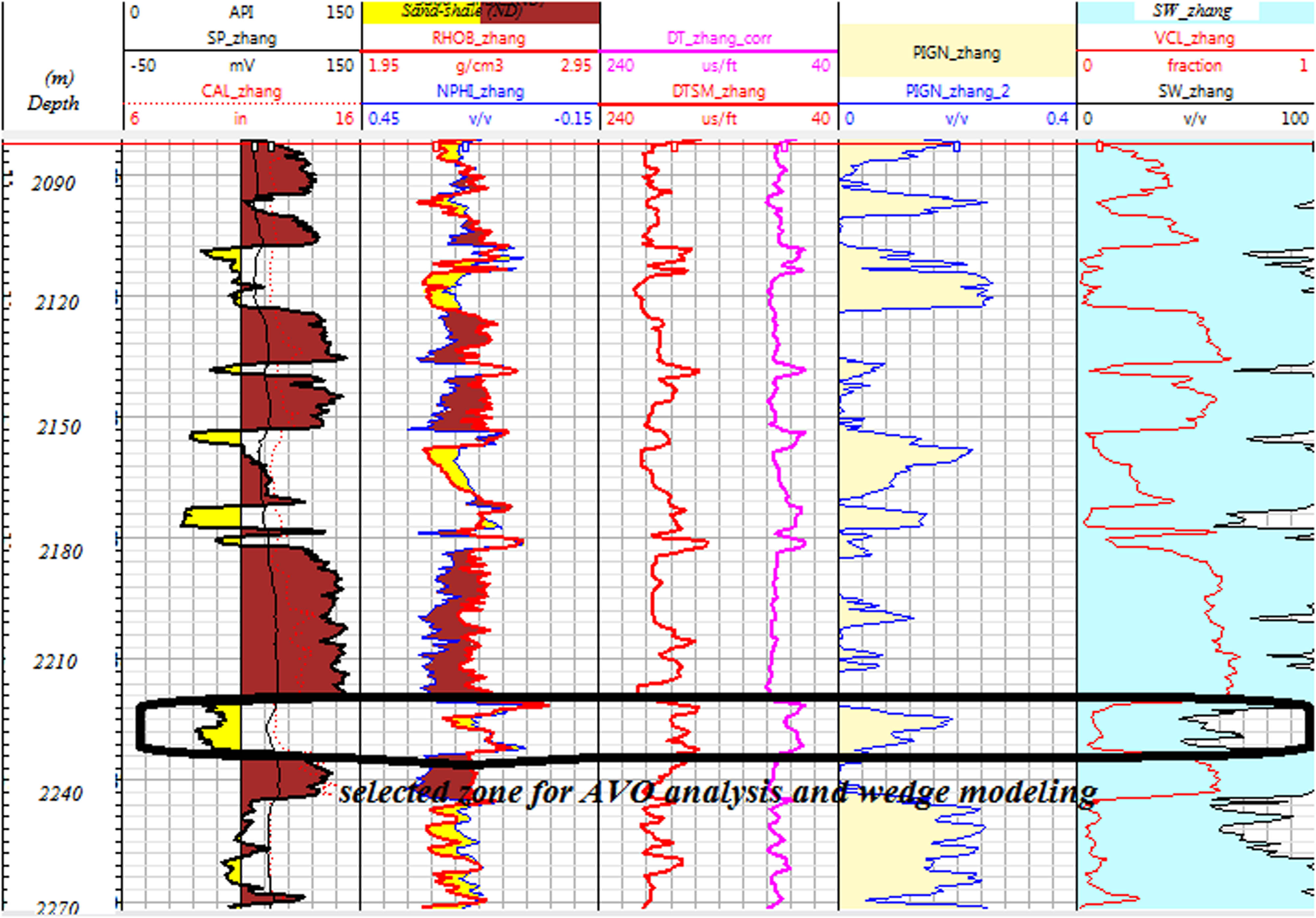
Composite log showing different thin bed reservoirs and marked zone which have been analyzed through AVO modeling.
3.2 Wedge modeling
Well log analyses clearly indicate that the Zhujiang Formation of Miocene age contains thin reservoir intervals (Figure 3); therefore, wedge modeling is carried out to estimate the seismic response with reference to thickness variation. A three-layer wedge model is developed in which a layer of limestone is embedded between two shale layers. The elastic values used to develop the double interference wedge model are given in Table 1.
The elastic parameters used to develop the three-layer wedge model for the selected interval
| Layers | Vp (m/s) | Vs (m/s) | Density (g/cm3) |
|---|---|---|---|
| 1 | 3,250 | 1,560 | 2.39 |
| 2 | 3,440 | 1,780 | 2.44 |
| 3 | 3,270 | 1,570 | 2.40 |
The tuning thickness is determined by using the following equation [52]:
where z is the tuning thickness of a bed, usually ¼ of the wavelength (λ⧸4), vi is the interval velocity of the target layer, and fd is the dominant frequency. The tuning thickness is calculated at 35, 40, and 45 Hz dominant frequencies, and the obtained results are shown in Figures 4–6, respectively.
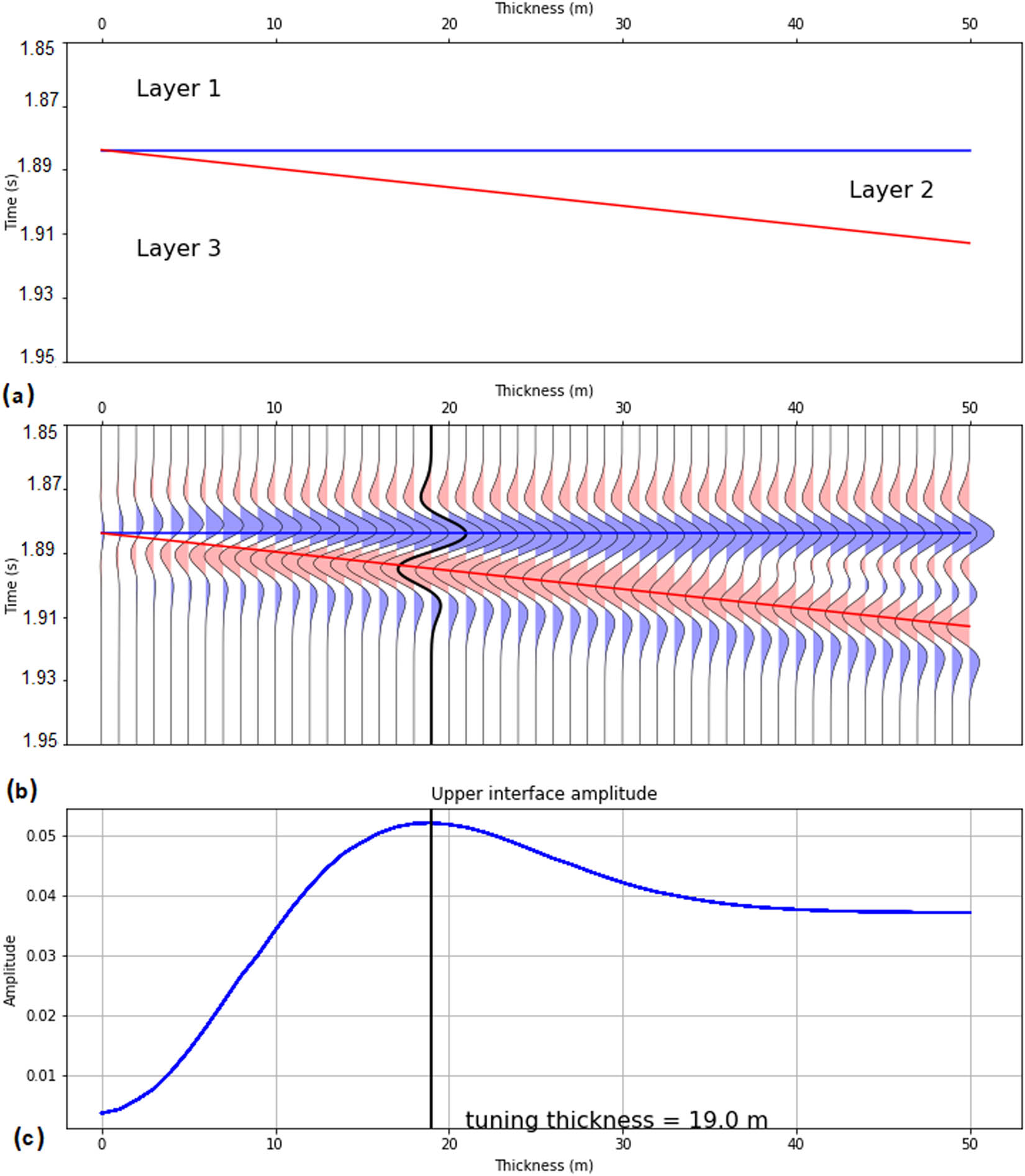
(a) Three-layer wedge model for selected interval. (b) Synthetic seismogram by using zero offset Ricker wavelet of 35 Hz frequency. (c) Amplitude of synthetic seismogram showing maximum response at 19 m thickness.
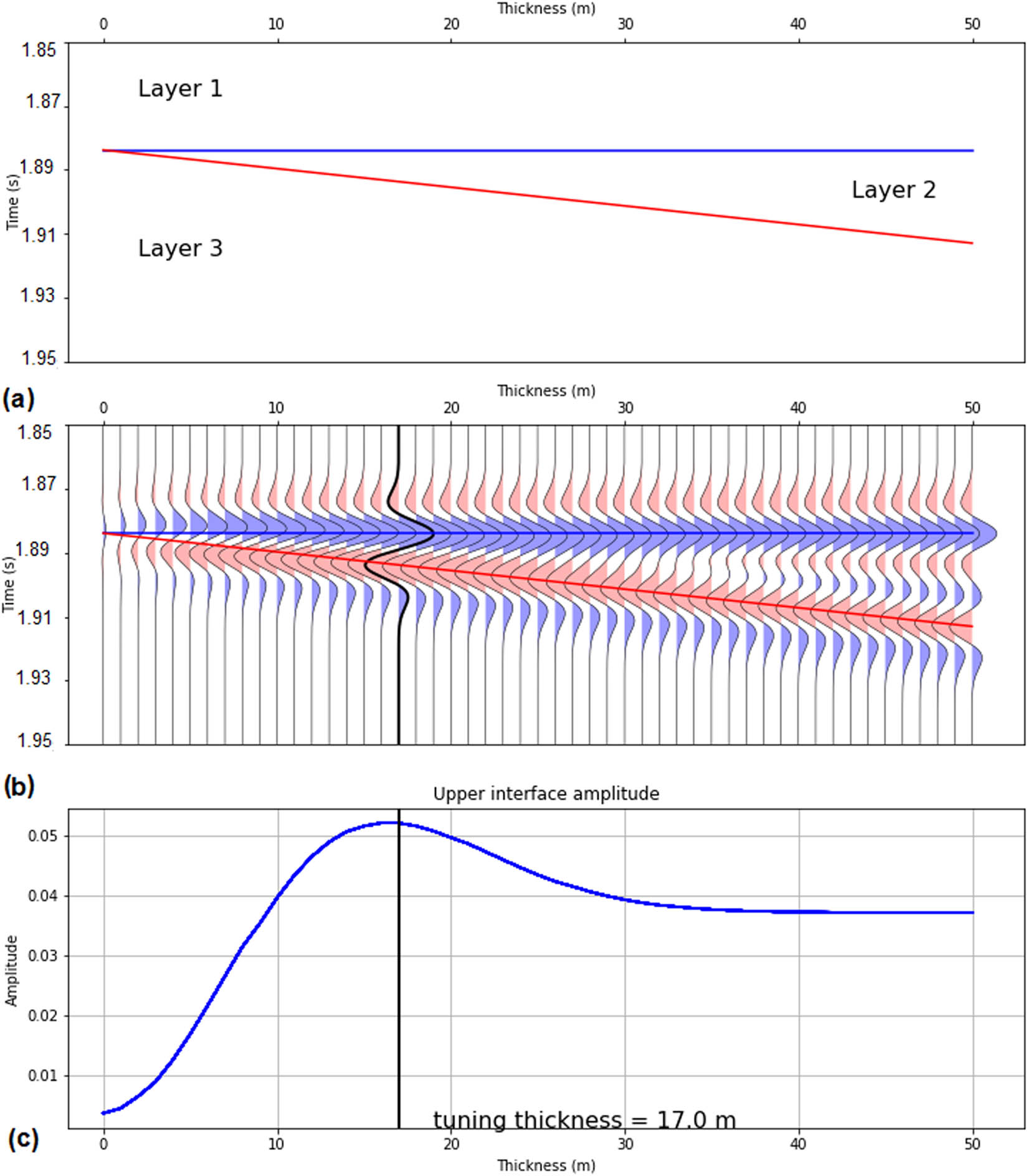
(a) Three-layer wedge model for selected interval. (b) Synthetic seismogram by using zero offset Ricker wavelet of 40 Hz frequency. (c) Amplitude of synthetic seismogram showing maximum response at 17 m thickness.
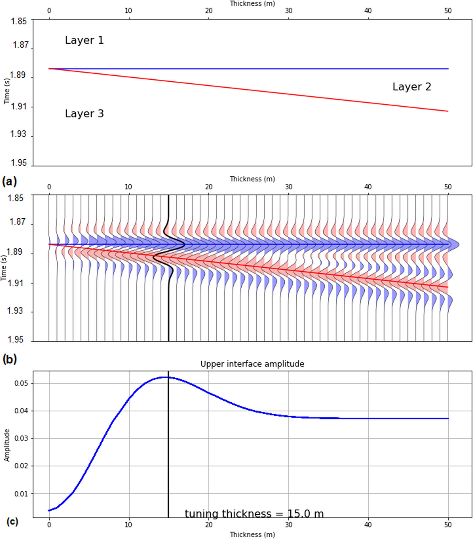
(a) Three-layer wedge model for selected interval. (b) Synthetic seismogram by using zero offset Ricker wavelet of 45 Hz frequency. (c) Amplitude of synthetic seismogram showing maximum response at 15 m thickness.
3.3 AVO analysis
The theory of AVO is based on the Zoeppritz equations, which give the plane wave reflection and transmission coefficients as a function of the angle of incidence and elastic parameters. The changes in elastic properties are useful indicators to infer the litho-fluid changes from one layer to another. In this study, exact Zoeppritz equations are used to analyze the variation in reflection coefficient concerning the incidence angle from the top and bottom of the target interval. The used exact Zoeppritz equations are given below [53].
where Rp is the P-wave reflection coefficient, Rs is the Sv-wave reflection coefficient, Tp is the P-wave transmitted amplitude, and Ts is the Sv-wave transmitted amplitude. In this equation, θ1, θ2 are the reflection angles and φ1, φ2 are the transmission angles for P- and Sv-wave, respectively. The P- and S-wave velocities and density of upper and lower half spaces are denoted by Vp1, Vs1, ρ1 and Vp2, Vs1, ρ2, respectively.
Although the Zoeppritz equation deals with the angle of incidence, in this study, we are more concerned to analyze the variations in thickness and their consequent effect on AVO response. In order to analyze the effect of thickness, we convolved the reflection coefficients obtained from the Zoeppritz equation with Ricker (source) wavelet. For convolving coefficients, we considered the two-way travel time because the change in thickness of the layer also effects the travel time values.
Finally, we have used Shuey’s [54] equation to estimate the value of intercept and gradient at different thicknesses. Then, these attributes are cross plotted to analyze the effect of thickness on AVO attributes. The used Shuey’s [54] equation can be expressed as follows:
with
R(0) is the reflection coefficients at the normal angle of incidence, also known as AVO intercept. B represents the AVO gradient and explains the variation in reflection amplitudes at an intermediate angle of incidence. The third term C is denoted as curvature and explains the behavior of reflection coefficients at far angles of incidence, sometimes close to the critical angle [55]. If we assume that the angle of incidence is less than 30°, Shuey’s equation is reduced to the two-term equation written as:
4 Results
On the basis of the petrophysical analysis, different hydrocarbon-bearing zones are identified, as shown in Figure 3. In these zones, the crossover between density and neutron porosity logs, decrease in volume of shale (less than 15%), water saturation (less than 50%), and increase in effective porosity (porosity values vary from 15 to 25%) suggest that these clean and porous zones are favorable for the accumulation of hydrocarbons. The thickness of these hydrocarbon bearing zones varies from 5 to 24 m (Figure 3). Hence, the petrophysical analysis clearly depicts that the Zhujiang Formation of Miocene age contains thin hydrocarbon-bearing beds that have been embedded between shale beds.
Since the thickness of the hydrocarbon intervals is below seismic resolution, it is not possible to accurately demarcate these thin intervals on seismic data. In the presence of thin beds, seismic waves from closely spaced boundaries exhibit single event of high amplitude, and consequently, these reflected waves will not reveal the actual response of the subsurface geology. The amplitude of seismic reflections also changes with the change in thickness of the bed [56]. Therefore, based on petrophysical analysis, we have chosen a reservoir interval, which has 15 m thickness favorable for hydrocarbon accumulation. A three-layer wedge model is constructed keeping in view the thickness of the reservoir zone, in which the carbonate layer is embedded between two shale layers (Figure 4a). The parameters used to construct the wedge model are listed in Table 1. The wedge model has a maximum thickness of 50 m. A zero-phase Ricker wavelet of 35 Hz frequency is convolved with the reflection coefficient in order to generate the synthetic traces (Figure 4b). The top of the wedge shows a positive impedance contrast, whereas the bottom shows a negative impedance contrast. Figure 4c indicates that the amplitude increases with the increase in thickness up to 19 m and then shows a decrease in amplitude up to 42 m thickness. However, when the thickness increases from 42 m, amplitude response becomes flat, which indicates that seismic reflections from the top and base of the wedge are not interfering.
From the above analysis, it is clear that the peak of seismic amplitudes can be observed at 19 m thickness, which means that at 35 Hz frequency, beds having a thickness of 19 m or above can be easily resolved on seismic data. A similar procedure is adapted for 40 and 45 Hz frequencies in order to analyze the variation in tuning thickness due to change in frequency values (Figures 5 and 6). Wedge model results illustrate that at 40 and 45 Hz frequencies carbonate beds having a thickness of 17 and 15 m can be easily resolved through seismic data, respectively.
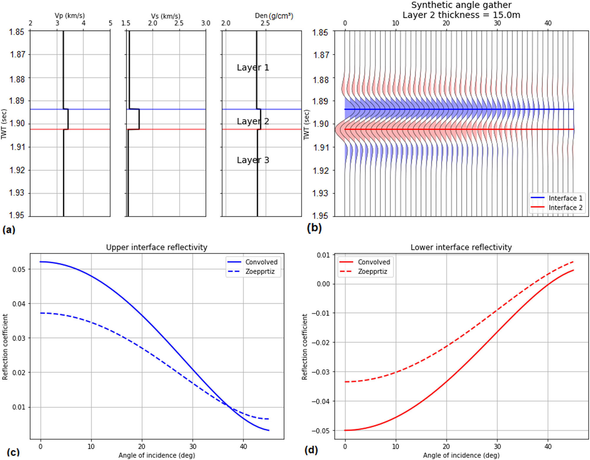
In the above discussion, we have analyzed the synthetic gathers at zero offset. Furthermore, synthetic angle gathers are examined in order to understand the effect of thin bed tuning on angle-dependent reflectivity. Angle-dependent reflectivities (amplitudes) along the top and bottom interfaces (Figure 7a and b) are estimated with the help of convolved and exact Zoeppritz equations considering the 19 m bed thickness (Figure 7c and d). The Zoeppritz equation explains the reflection of plane waves coming from a single interface, which does not contain potential information about the reflection responses of thin layers [20]. Therefore, we have also considered the convolved amplitudes to understand the reflection response of thin layers. Figure 7c (upper interface) shows that at zero angle, the value of convolved amplitudes is much higher than the Zoeppritz, and both values gradually decrease with the increase in the angle of incidence. However, the value of convolved amplitudes decreases more rapidly than the Zoeppritz amplitudes crossing its reflectivities at an angle of 32 degrees. After that angle, the convolved amplitudes become smaller than the Zoeppritz reflectivity, which may indicate a destructive interference. On the other hand, the reflectivities along the lower interface are the converse of the top interface (Figure 7d). The gap between these amplitudes curves also decreases with the increase in the angle of incidence; however, these two reflectivity curves (convolved and Zoeppritz) do not intersect each other.
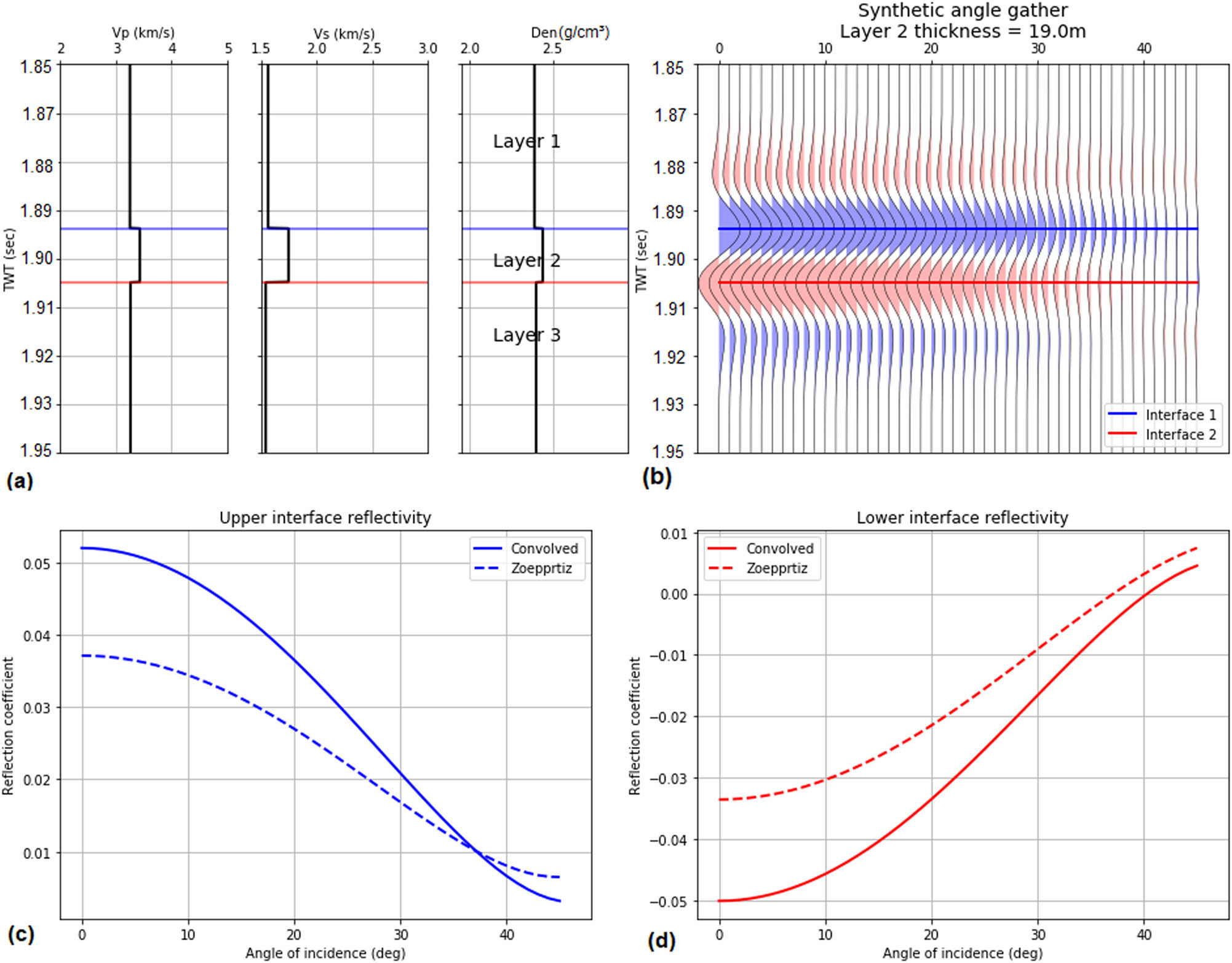
(a) Reflectivity response of elastic parameters for selected interval. (b) Synthetic angle gathers considering the 19 m bed thickness. (c) Angle-dependent reflectivities (amplitude) estimated with convolved and standard Zoeppritz equations of the upper interface. (d) Angle-dependent reflectivities (amplitude) estimated with convolved and standard Zoeppritz equations of the lower interface.
To further analyze the behavior of angle-dependent reflectivity, we have computed the reflectivity responses for 14 and 24 m thicknesses (considering 5 m above and below the tuning thickness), keeping the other parameters same as used for Figure 7. The computed results are shown in Figures 8 and 9, respectively. The obtained results depict that at 14 m thickness (Figure 8b) top and bottom interfaces do not pass through the center of the peak and trough of the synthetic, respectively. It means that at this thickness, the maximum values of amplitudes (reflectivity) cannot be obtained. Figure 8c and d also show a decrease in convolved amplitudes as compared to Figure 7c and d. However, reflectivity values computed from the exact Zoeppritz equation do not show any change. Hence, at 14 m thickness, the obtained reflectivity values are lower than those values which we have obtained at 19 m thickness. So, at 14 m thickness (at a frequency of 35 Hz) AVO results cannot accurately interpret the tuning phenomena. Similarly, results obtained at 24 m thickness also show a decrease in convolved amplitude values, but in this case, top and bottom interfaces move apart from each other (Figure 9). So from the above discussion, it is obvious that at 35 Hz frequency AVO analysis provides more reliable results for 19 m thin bed.
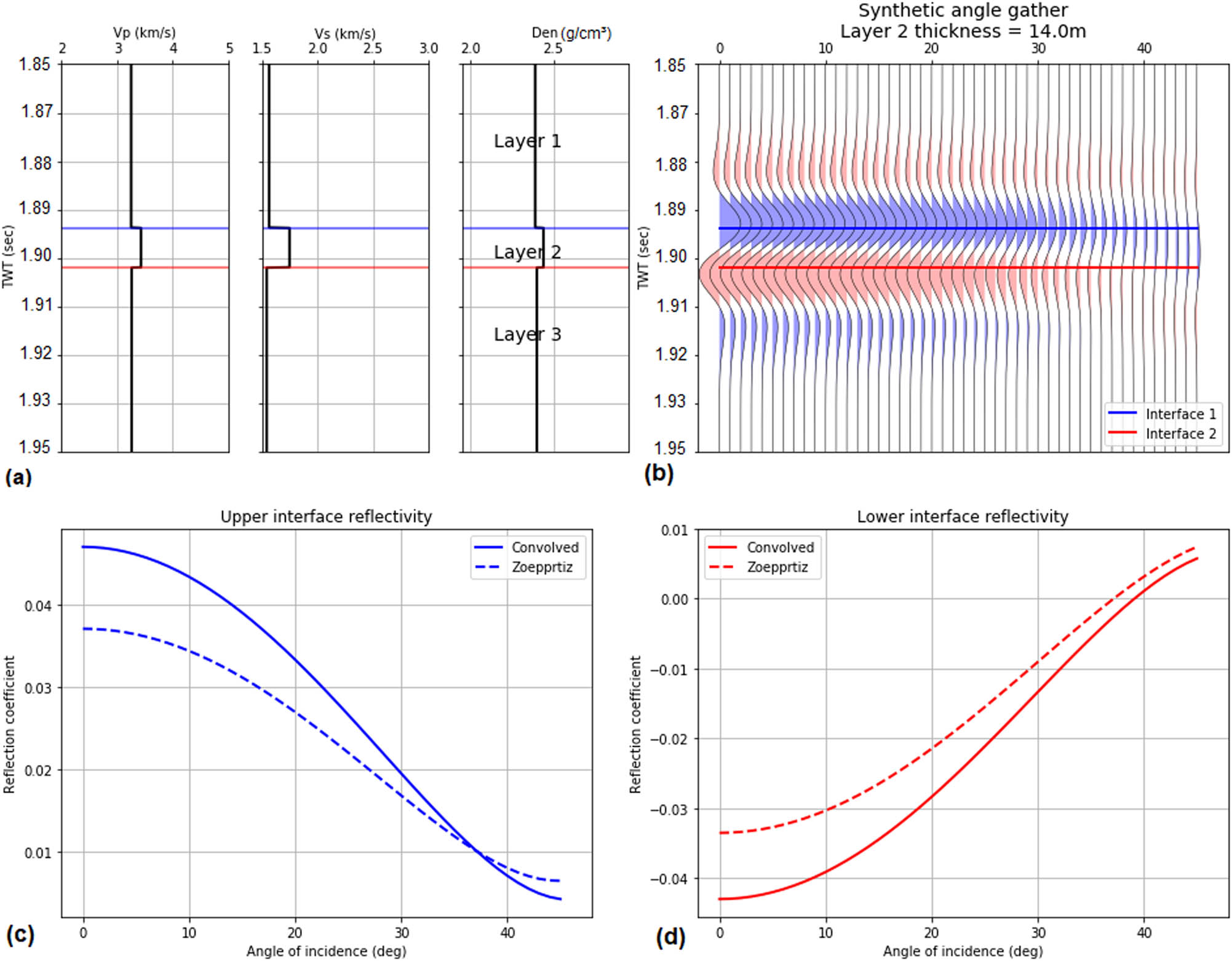
(a) Reflectivity response of elastic parameters for selected interval. (b) Synthetic angle gathers considering the 14 m bed thickness. (c) Angle-dependent reflectivities (amplitude) estimated with convolved and standard Zoeppritz equations of the upper interface. (d) Angle-dependent reflectivities (amplitude) estimated with convolved and standard Zoeppritz equations of the lower interface.
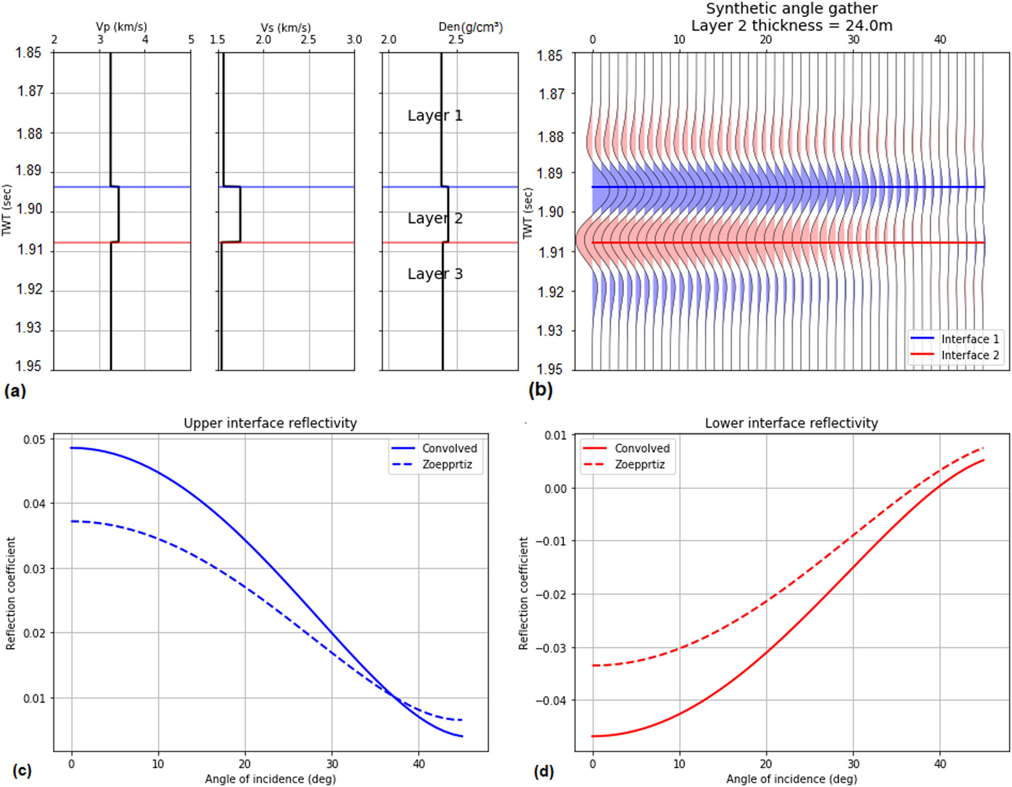
(a) Reflectivity response of elastic parameters for selected interval. (b) Synthetic angle gathers considering the 24 m bed thickness. (c) Angle-dependent reflectivities (amplitude) estimated with convolved and standard Zoeppritz equations of the upper interface. (d) Angle-dependent reflectivities (amplitude) estimated with convolved and standard Zoeppritz equations of the lower interface.
Similarly, we have performed AVO analysis for 17 and 15 m thicknesses considering the 40 and 45 Hz frequencies, respectively. The obtained results are shown in Figures 10 and 11. From these results (Figures 10 and 11), it is quite clear that reflectivity responses obtained along the top and bottom interfaces are identical to those reflectivities which we have obtained for 19 m thickness at 35 Hz frequency (Figure 7). We also have computed reflectivity response considering the thickness values 5 m above and below the tuning thickness values, i.e., at 12 and 22 m, (for 40 Hz frequency), 10 and 20 m (for 45 Hz frequency). The obtained results are shown in Figures 12–15, respectively. Again, it is evident that the AVO responses obtained for 12 and 10 m thicknesses (Figures 12 and 14) are identical to what we have observed in Figure 8 and the AVO responses obtained for 22 and 20 m thicknesses (Figures 13 and 15) are identical to Figure 9. It means that the AVO response at different tuning thicknesses (19, 17, and 15 m) does not change, provided that the other parameters remain same except frequency.
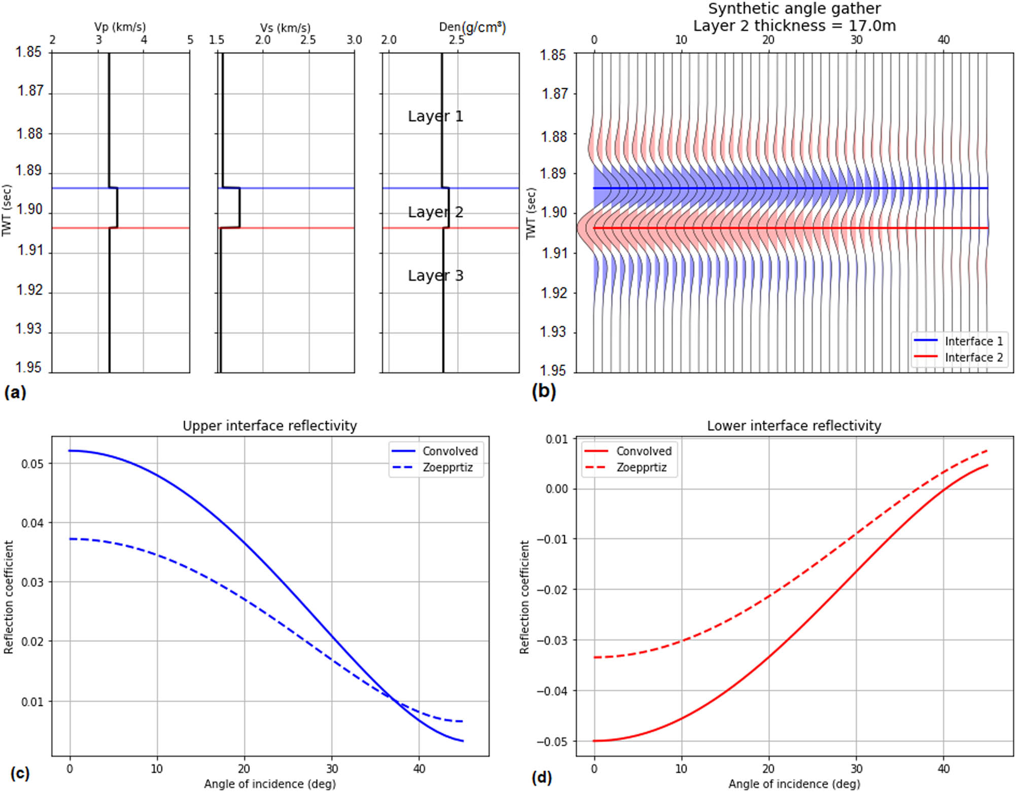
(a) Reflectivity response of elastic parameters for selected interval. (b) Synthetic angle gathers considering the 17 m bed thickness. (c) Angle-dependent reflectivities (amplitude) estimated with convolved and standard Zoeppritz equations of the upper interface. (d) Angle-dependent reflectivities (amplitude) estimated with convolved and standard Zoeppritz equations of the lower interface.
(a) Reflectivity response of elastic parameters for selected interval .(b) Synthetic angle gathers considering the 15 m bed thickness. (c) Angle-dependent reflectivities (amplitude) estimated with convolved and standard Zoeppritz equations of the upper interface. (d) Angle-dependent reflectivities (amplitude) estimated with convolved and standard Zoeppritz equations of the lower interface.

(a) Reflectivity response of elastic parameters for selected interval. (b) Synthetic angle gathers considering the 12 m bed thickness. (c) Angle-dependent reflectivities (amplitude) estimated with convolved and standard Zoeppritz equations of the upper interface. (d) Angle-dependent reflectivities (amplitude) estimated with convolved and standard Zoeppritz equations of the lower interface.
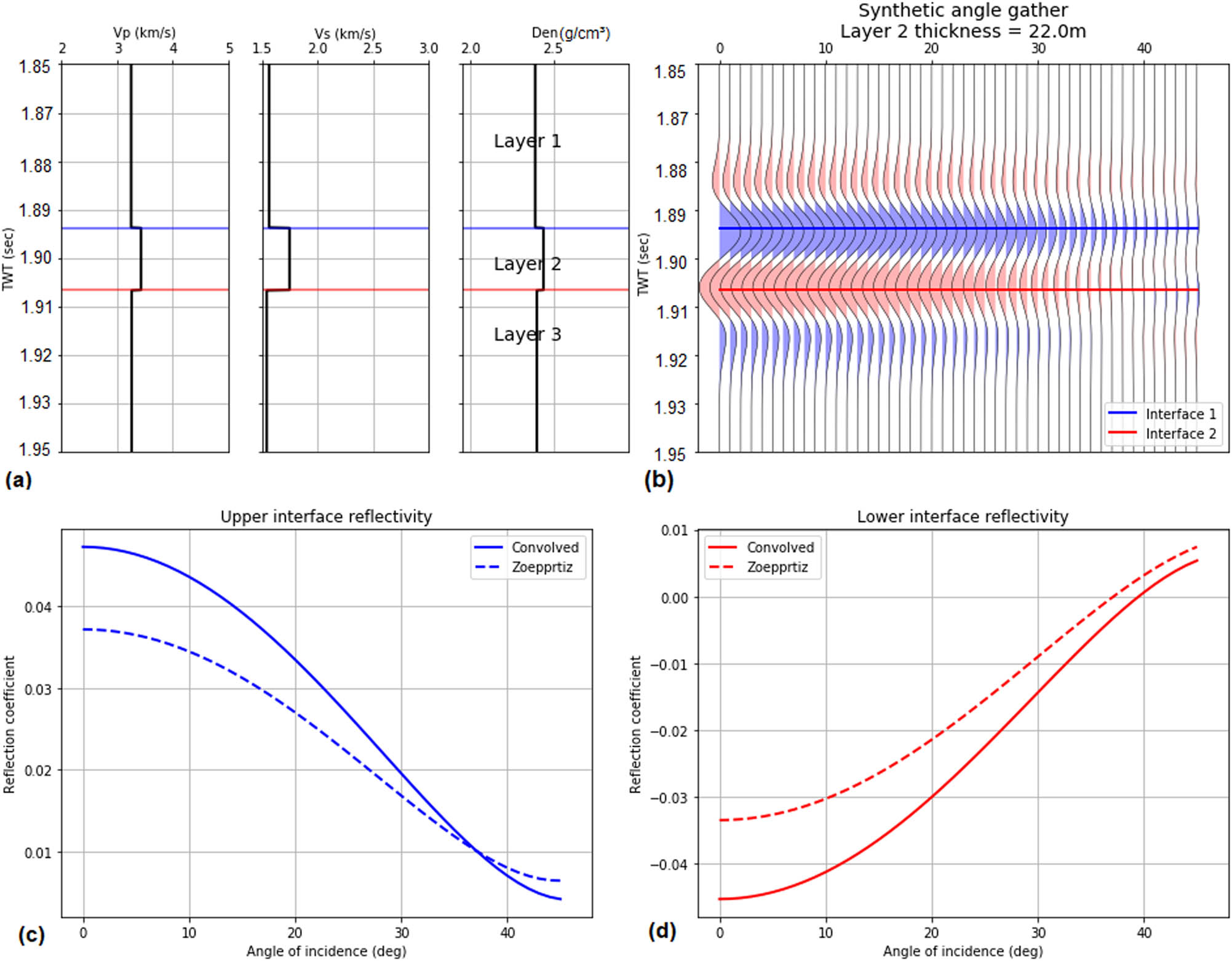
(a) Reflectivity response of elastic parameters for selected interval. (b) Synthetic angle gathers considering the 22 m bed thickness. (c) Angle-dependent reflectivities (amplitude) estimated with convolved and standard Zoeppritz equations of the upper interface. (d) Angle-dependent reflectivities (amplitude) estimated with convolved and standard Zoeppritz equations of the lower interface.
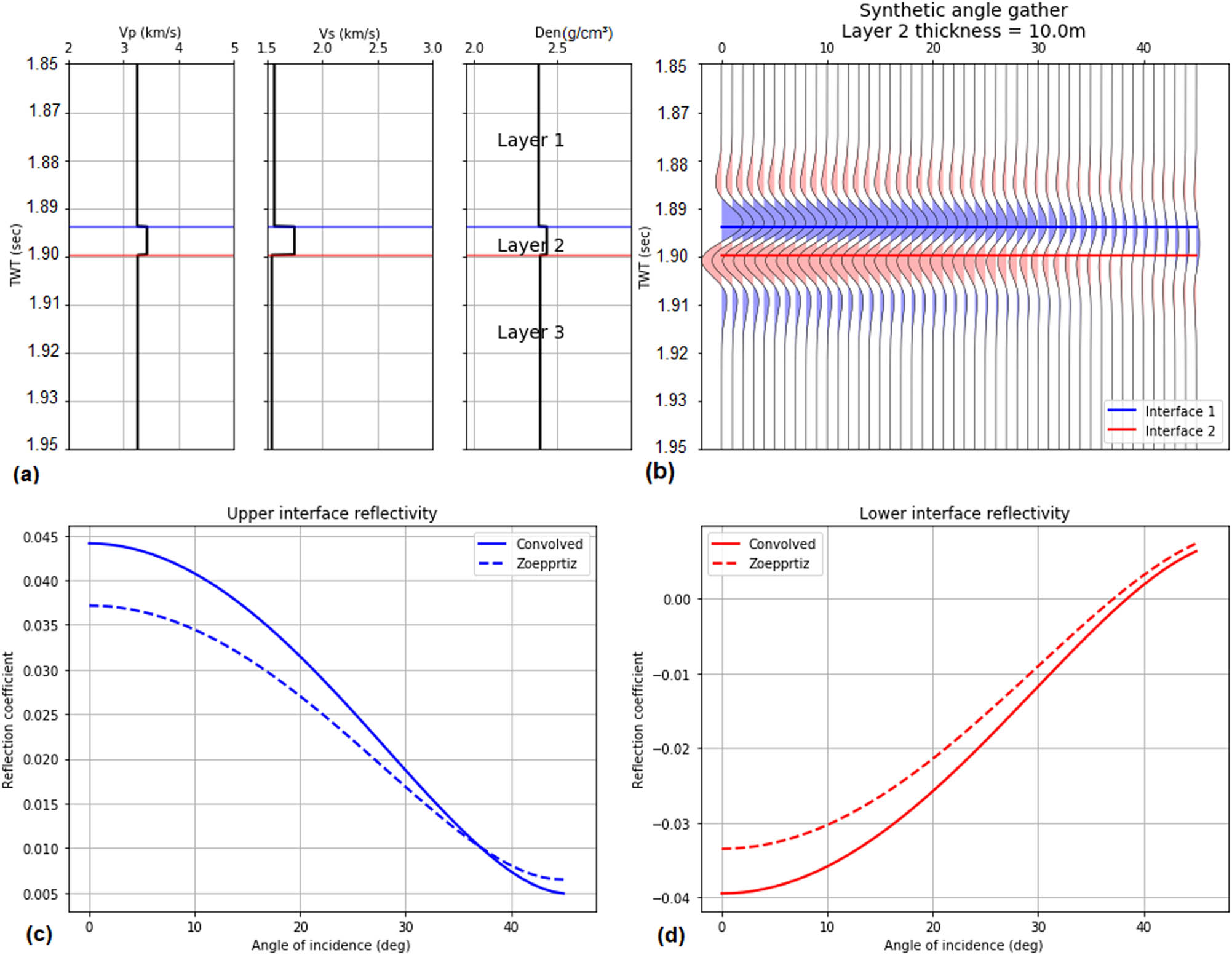
(a) Reflectivity response of elastic parameters for selected interval. (b) Synthetic angle gathers considering the 10 m bed thickness. (c) Angle-dependent reflectivities (amplitude) estimated with convolved and standard Zoeppritz equations of the upper interface. (d) Angle-dependent reflectivities (amplitude) estimated with convolved and standard Zoeppritz equations of the lower interface.

(a) Reflectivity response of elastic parameters for selected interval. (b) Synthetic angle gathers considering the 20 m bed thickness. (c) Angle-dependent reflectivities (amplitude) estimated with convolved and standard Zoeppritz equations of the upper interface. (d) Angle-dependent reflectivities (amplitude) estimated with convolved and standard Zoeppritz equations of the lower interface.
AVO attributes (intercept and gradient) are considered a powerful tool to analyze the thin bed tuning. The values of intercept and gradient are calculated for the top interface with the help of Shuey’s two-term equation (equation (9)) considering different thickness values. Values of intercept increase with the increase in thickness and attain their peak values at 15, 17, and 19 m thickness for 45, 40, and 35 Hz frequencies, respectively (Figure 16a). After that, intercept values gradually decrease with the increase in bed thickness and become almost flat after 35 m thickness. A mirror image of Figure 16a is obtained for a cross plot of gradient versus thickness with a negative increase in gradient values (Figure 16b). It means that the values of intercept and gradient attain their peak value at λ/4, which represents tuning thickness at their respective frequencies and also cross validate the results obtained with the help of equation (6).
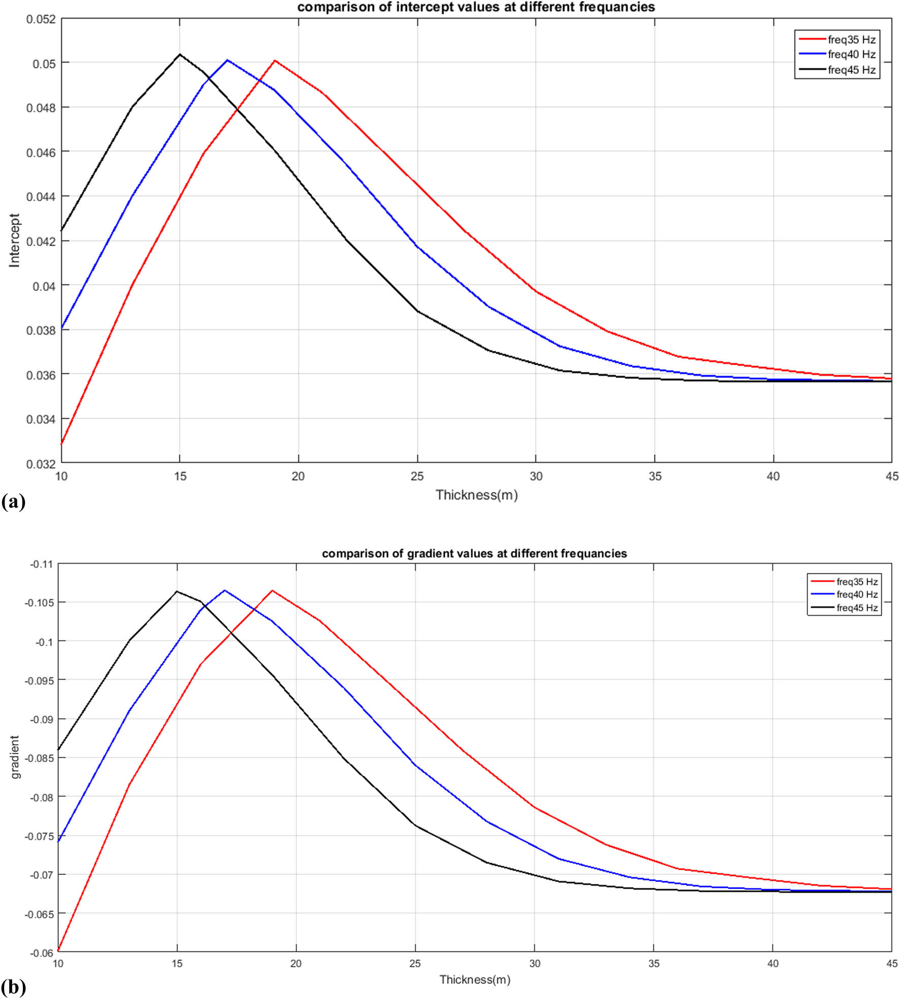
(a) Variation in intercept values with respect to thickness at different frequencies (30 Hz, red color; 40 Hz, blue color; and 45 Hz, black color). (b) Variation in gradient values with respect to thickness at different frequencies (30 Hz, red color; 40 Hz, blue color; and 45 Hz, black color).
5 Conclusions
In this work, the quantitative seismic response of thin limestone beds of the Zhujiang Formation is studied by integrating petrophysics, wedge modeling, and three-layer AVO modeling. The petrophysical analysis depicts that the Zhujiang Formation of Miocene age contains thin (5–24 m) hydrocarbon-rich limestone intervals. Through wedge modeling, it is observed that the beds having a thickness of 19, 17, and 15 m can be resolved if the acquired seismic data have a dominant frequency of 35, 40, and 45 Hz, respectively. AVO results show that convolved amplitudes show clear variations in AVO response at different thickness values, whereas Zoeppritz results remain unchanged. Convolved amplitudes provide maximum values at tuning thickness (at a particular frequency), whereas the value of convolved amplitudes decrease above and below the tuning thickness. Furthermore, AVO attributes also validate the wedge modeling results and show the decreasing trend after the tuning thickness.
Acknowledgments
The authors would like to acknowledge the National Natural Science Foundation of China for substantial support of general projects (41374116 and 41674113), Chinese National Offshore Oil Company for providing well log data used in this research, and Chinese Scholarship Council. We would also be thankful to Mat Hall for providing open-access python script and for valuable guidance for this work.
Conflict of interest: The authors declare no conflict of interest.
References
[1] Chi X, Han D. Lithology and fluid differentiation using a rock physics template. Lead Edge. 2009;28(1):60–5.10.1190/1.3064147Search in Google Scholar
[2] Dubey AK. Student FYIMS. Reservoir characterization using AVO and seismic inversion techniques; 2012.Search in Google Scholar
[3] Azeem T, Chun WY, Lisa M, Khalid P, Qing LX, Ehsan MI, et al. An integrated petrophysical and rock physics analysis to improve reservoir characterization of Cretaceous sand intervals in Middle Indus Basin, Pakistan. J Geophys Eng. 2017;14:212–25.10.1088/1742-2140/14/2/212Search in Google Scholar
[4] Farfour M, Yoon WJ, Kim J. Seismic attributes and acoustic impedance inversion in interpretation of complex hydrocarbon reservoirs. J Appl Geophys. 2015;114:68–80.10.1016/j.jappgeo.2015.01.008Search in Google Scholar
[5] Ricker N. Wavelet contraction, wavelet expansion, and the control of seismic resolution. Geophysics. 1953;18:769–92.10.1190/1.1437927Search in Google Scholar
[6] Widess M. How thin is a thin bed? Geophysics. 1973;38:1176–80.10.1190/1.1440403Search in Google Scholar
[7] Chopra S, Alexeev V. Applications of texture attribute analysis to 3D seismic data. Lead Edge. 2006;25:934–40.10.1190/1.2144439Search in Google Scholar
[8] Liu Y, Schmitt DR. Amplitude and AVO responses of a single thin bed. Geophysics. 2003;68:1161–8.10.1190/1.1598108Search in Google Scholar
[9] Othman AA, Fathy M, Maher A. Use of spectral decomposition technique for delineation of channels at solar gas discovery, offshore West Nile Delta, Egypt. Egypt J Pet. 2016;25:45–51.10.1016/j.ejpe.2015.03.005Search in Google Scholar
[10] Puryear CI, Castagna JP. Layer-thickness determination and stratigraphic interpretation using spectral inversion: Theory and application. Geophysics. 2008;73:R37–R48.10.1190/1.2838274Search in Google Scholar
[11] Castagna JP, Backus MM. Offset-dependent reflectivity–Theory and practice of AVO analysis: Society of Exploration Geophysicists; 1993.10.1190/1.9781560802624Search in Google Scholar
[12] Castagna JP, Smith SW. Comparison of AVO indicators: A modeling study. Geophysics. 1994;59:1849–55.10.1190/1.1822603Search in Google Scholar
[13] Castagna JP, Swan HW, Foster DJ. Framework for AVO gradient and intercept interpretation. Geophysics. 1998;63:948–56.10.1190/1.1444406Search in Google Scholar
[14] Ali A, Alves TM, Rehman K. The accuracy of AVA approximations in isotropic media assessed via synthetic numerical experiments: implications for the determination of porosity. J Pet Sci Eng. 2018;170:563–75.10.1016/j.petrol.2018.06.082Search in Google Scholar
[15] Ostrander W. Plane-wave reflection coefficients for gas sands at nonnormal angles of incidence. Geophysics. 1984;49:1637–48.10.1190/1.1826898Search in Google Scholar
[16] Ursin B, Dahl T. Seismic reflection amplitudes. Geophys Prospect. 1992;40:483–512.10.1111/j.1365-2478.1992.tb00538.xSearch in Google Scholar
[17] Hilterman FJ. Seismic amplitude interpretation: Society of Exploration Geophysicists and European Association of; 2001.10.1190/1.9781560801993Search in Google Scholar
[18] Veeken P, Rauch-Davies M, Gallardo R, Villasenor RV, Macuspana P, Tebar DC. Model-driven inversion of the Fortuna National 3D seismic data in the Macuspana Basin, onshore Mexico. SEG Technical Program Expanded Abstracts 2002: Society of Exploration Geophysicists; 2002. p. 898–901.10.1190/1.1817407Search in Google Scholar
[19] Da Silva M, Rauch-Davies M, Cuervo AS, Veeken P. Data conditioning for a combined inversion and AVO reservoir characterisation study. 66th EAGE Conference & Exhibition; 2004.10.3997/2214-4609-pdb.3.P306Search in Google Scholar
[20] Pan W, Innanen KA. AVO/AVF analysis of thin beds in elastic media. SEG Technical Program Expanded Abstracts 2013: Society of Exploration Geophysicists; 2013. p. 373–7.10.1190/segam2013-0587.1Search in Google Scholar
[21] Li Y, Downton J, Xu Y. Practical aspects of AVO modeling. Lead Edge. 2007;26:295–311.10.1190/1.2715053Search in Google Scholar
[22] Peng S, Gao Y. Study on the AVO forward modeling of coal bearing strata. Chin Sci Bull. 2005;50:151–8.10.1007/BF03184099Search in Google Scholar
[23] Yuan T, Hyndman R, Spence G, Desmons B. Velocity structure of a bottom-simulating reflector and deep sea gas hydrate concentrations on the Cascadia continental slope. J Geophys Res. 1996;101:13655–71.10.1029/96JB00102Search in Google Scholar
[24] Wang Z. Feasibility of time-lapse seismic reservoir monitoring: The physical basis. Lead Edge. 1997;16:1327–30.10.1190/1.1437796Search in Google Scholar
[25] De Voogd N, Den Rooijen H. Thin-layer response and spectral bandwidth. Geophysics. 1983;48:12–8.10.1190/1.1441400Search in Google Scholar
[26] Gochioco LM. Tuning effect and interference reflections from thin beds and coal seams. Geophysics. 1991;56:1288–95.10.1190/1.1443151Search in Google Scholar
[27] Kallweit R, Wood L. The limits of resolution of zero-phase wavelets. Geophysics. 1982;47:1035–46.10.1190/1.1441367Search in Google Scholar
[28] Chung H, Lawton D. Frequency characteristics of seismic reflections from thin beds. Can J Explor Geophys. 1995;31:32–7.Search in Google Scholar
[29] Rutherford SR, Williams RH. Amplitude-versus-offset variations in gas sands. Geophysics. 1989;54:680–8.10.1190/1.1442696Search in Google Scholar
[30] Castagna JP, Batzle ML, Eastwood RL. Relationships between compressional-wave and shear-wave velocities in clastic silicate rocks. Geophysics. 1985;50:571–81.10.1190/1.1441933Search in Google Scholar
[31] Feng H, Bancroft JC. AVO principles, processing and inversion. CREWES Res Rep. 2006;18:1–19.Search in Google Scholar
[32] Leyla BH, Zhang J, Yang L. Quantitative Analysis of Faults in Huizhou Sub-basin, Pearl River Mouth Basin. J Earth Sci. 2018;29:169–81.10.1007/s12583-018-0823-3Search in Google Scholar
[33] Tang X, Yang S, Zhu J, Long Z, Jiang G, Huang S, et al. Tectonic subsidence of the Zhu 1 Sub-basin in the Pearl River Mouth Basin, northern South China Sea. Front Earth Sci. 2017;11:729–39.10.1007/s11707-016-0610-3Search in Google Scholar
[34] Chimney P, Lomando A, Popek J. Trap and seal analysis in carbonate shelf margin stratigraphic trap exploration; example from the lower Miocene, Zhujiang Fm., Pearl River Mouth Basin, People’s Republic of China. AAPG Bull. 1996;5.Search in Google Scholar
[35] Lin C, Zhang Y. Modeling analysis of basin depression history. Continental margin basin analysis and hydrocarbon accumulation of the Northern South China Sea. China Beijing: Science Press; 1997.Search in Google Scholar
[36] Zhou D. Studies in the Tectonics of China: Extensional Tectonics of the Northern Margin of the South China Sea; Amalgamation and Uplift of the Tian Shan; and Wedge Extrusion Model for the Altyn Tagh Fault; 1997.Search in Google Scholar
[37] Holloway N. North Palawan block, Philippines–Its relation to Asian mainland and role in evolution of South China Sea. AAPG Bull. 1982;66:1355–83.10.7186/bgsm14198102Search in Google Scholar
[38] Wang R, Deng H, Li S. The Paleogene sequence stratigraphy and sedimentary system research in the Zhu 1 Depression in Pearl River Mouth Basin. Pet Geol Recovery Effic. 2009;16:4–7.Search in Google Scholar
[39] Cheng T, Wang Z, Zhang S, Liu J. Research on high-resolution sequence stratigraphy of marine-continental alternating fades delta-taking Zhuhai Formation in Huizhou Sag. Pearl River Mouth Basin as an example. Pet Geol Recovery Effic. 2007;14:46–51.Search in Google Scholar
[40] Yun L, Rongcai Z, Baoquan Y, Guojin Z, Boyu G, Xiaoqing H. Deep-water Depositional Features of Miocene Zhujiang Formation in Baiyun Sag, Pearl River Mouth Basin. Acta Geol Sin (Engl Ed). 2013;87:197–210.10.1111/1755-6724.12041Search in Google Scholar
[41] Jiang H, Pang X, Shi H, Liu L, Bai J, Zou S. Effects of fault activities on hydrocarbon migration and accumulation in the Zhu I Depression, Pearl River Mouth Basin, South China Sea. Aust J Earth Sci. 2015;62:775–88.Search in Google Scholar
[42] Gong ZS, Li ST, Xie T, et al. Continental margin basin analysis and hydrocarbon accumulation of the northern South China Sea. Beijing: China Sci Press; 1997. p. 510, (in Chinese).Search in Google Scholar
[43] Sattler U, Immenhauser A, Schlager W, Zampetti V. Drowning history of a Miocene carbonate platform (Zhujiang Formation, South China Sea). Sediment Geol. 2009;219:318–31.10.1016/j.sedgeo.2009.06.001Search in Google Scholar
[44] Bisht BS, Sas SK, Chaudhuri PK, Song RBN, Singh SK. Integration of petrophysics and rock-physics modeling in single workflow reduces uncertainty in seismic reservoir characterization: a case study. Geohorizons. 2013;44–7.Search in Google Scholar
[45] Ali A, Kashif M, Hussain M, Siddique J, Aslam I, Ahmed Z. An integrated analysis of petrophysics, cross-plots and Gassmann fluid substitution for characterization of Fimkassar area, Pakistan: a case study. Arab J Sci Eng. 2015;40:181–93.10.1007/s13369-014-1500-1Search in Google Scholar
[46] Adeoti L, Ayolabi E, James P. An integrated approach to volume of shale analysis: Niger Delta example, Offrire Field. World Appl Sci J. 2009;7:448–52.Search in Google Scholar
[47] Stieber S. Pulsed neutron capture log evaluation-louisiana gulf coast. Fall Meeting of the Society of Petroleum Engineers of AIME; 1970: Society of Petroleum Engineers.10.2118/2961-MSSearch in Google Scholar
[48] Archie GE. The electrical resistivity log as an aid in determining some reservoir characteristics. Soc Pet Eng J. 1942;146(1):54–62, SPE-942054-G.10.2118/942054-GSearch in Google Scholar
[49] Asquith GB, Krygowski D, Henderson S, Hurley N. Geologists AAoP. Basic Well Log Analysis: American Association of Petroleum Geologists; 2004.10.1306/Mth16823Search in Google Scholar
[50] Maute R, Lyle W, Sprunt ES. Improved data-analysis method determines archie parameters from core data (includes associated paper 24964). J Pet Technol. 1992;44:103–7.10.2118/19399-PASearch in Google Scholar
[51] Rider MH. The Geological Interpretation of Well Logs: Rider-French Consulting; 2002.Search in Google Scholar
[52] Sunjay S. GeoCanada 2010-Working with the Earth 1 Wavelets Transforms: Time-Frequency Presentation. 2010.Search in Google Scholar
[53] Zoeppritz K. On the reflection and propagation of seismic waves. Gottinger Nachrichten. 1919;1:66–84.Search in Google Scholar
[54] Shuey R. A simplification of the Zoeppritz equations. Geophysics. 1985;50:609–14.10.1190/1.1441936Search in Google Scholar
[55] Sheriff RE, Geldart LP. Exploration seismology. Cambridge university press; 1995.10.1017/CBO9781139168359Search in Google Scholar
[56] McArdle N, Ackers M. Understanding seismic thin-bed responses using frequency decomposition and RGB blending. First Break. 2012;30:57–65.10.3997/1365-2397.2012022Search in Google Scholar
[57] Pang X, Chen C-M, Shi H-S, et al. Response between relative sea-level change and the Pearl River deep-water fan system in the South China Sea. Dixue Qianyuan(Earth Sci Front). 2005;12:167–77.Search in Google Scholar
© 2020 Wasif Saeed et al., published by De Gruyter
This work is licensed under the Creative Commons Attribution 4.0 International License.
Articles in the same Issue
- Regular Articles
- The simulation approach to the interpretation of archival aerial photographs
- The application of137Cs and210Pbexmethods in soil erosion research of Titel loess plateau, Vojvodina, Northern Serbia
- Provenance and tectonic significance of the Zhongwunongshan Group from the Zhongwunongshan Structural Belt in China: insights from zircon geochronology
- Analysis, Assessment and Early Warning of Mudflow Disasters along the Shigatse Section of the China–Nepal Highway
- Sedimentary succession and recognition marks of lacustrine gravel beach-bars, a case study from the Qinghai Lake, China
- Predicting small water courses’ physico-chemical status from watershed characteristics with two multivariate statistical methods
- An Overview of the Carbonatites from the Indian Subcontinent
- A new statistical approach to the geochemical systematics of Italian alkaline igneous rocks
- The significance of karst areas in European national parks and geoparks
- Geochronology, trace elements and Hf isotopic geochemistry of zircons from Swat orthogneisses, Northern Pakistan
- Regional-scale drought monitor using synthesized index based on remote sensing in northeast China
- Application of combined electrical resistivity tomography and seismic reflection method to explore hidden active faults in Pingwu, Sichuan, China
- Impact of interpolation techniques on the accuracy of large-scale digital elevation model
- Natural and human-induced factors controlling the phreatic groundwater geochemistry of the Longgang River basin, South China
- Land use/land cover assessment as related to soil and irrigation water salinity over an oasis in arid environment
- Effect of tillage, slope, and rainfall on soil surface microtopography quantified by geostatistical and fractal indices during sheet erosion
- Validation of the number of tie vectors in post-processing using the method of frequency in a centric cube
- An integrated petrophysical-based wedge modeling and thin bed AVO analysis for improved reservoir characterization of Zhujiang Formation, Huizhou sub-basin, China: A case study
- A grain size auto-classification of Baikouquan Formation, Mahu Depression, Junggar Basin, China
- Dynamics of mid-channel bars in the Middle Vistula River in response to ferry crossing abutment construction
- Estimation of permeability and saturation based on imaginary component of complex resistivity spectra: A laboratory study
- Distribution characteristics of typical geological relics in the Western Sichuan Plateau
- Inconsistency distribution patterns of different remote sensing land-cover data from the perspective of ecological zoning
- A new methodological approach (QEMSCAN®) in the mineralogical study of Polish loess: Guidelines for further research
- Displacement and deformation study of engineering structures with the use of modern laser technologies
- Virtual resolution enhancement: A new enhancement tool for seismic data
- Aeromagnetic mapping of fault architecture along Lagos–Ore axis, southwestern Nigeria
- Deformation and failure mechanism of full seam chamber with extra-large section and its control technology
- Plastic failure zone characteristics and stability control technology of roadway in the fault area under non-uniformly high geostress: A case study from Yuandian Coal Mine in Northern Anhui Province, China
- Comparison of swarm intelligence algorithms for optimized band selection of hyperspectral remote sensing image
- Soil carbon stock and nutrient characteristics of Senna siamea grove in the semi-deciduous forest zone of Ghana
- Carbonatites from the Southern Brazilian platform: I
- Seismicity, focal mechanism, and stress tensor analysis of the Simav region, western Turkey
- Application of simulated annealing algorithm for 3D coordinate transformation problem solution
- Application of the terrestrial laser scanner in the monitoring of earth structures
- The Cretaceous igneous rocks in southeastern Guangxi and their implication for tectonic environment in southwestern South China Block
- Pore-scale gas–water flow in rock: Visualization experiment and simulation
- Assessment of surface parameters of VDW foundation piles using geodetic measurement techniques
- Spatial distribution and risk assessment of toxic metals in agricultural soils from endemic nasopharyngeal carcinoma region in South China
- An ABC-optimized fuzzy ELECTRE approach for assessing petroleum potential at the petroleum system level
- Microscopic mechanism of sandstone hydration in Yungang Grottoes, China
- Importance of traditional landscapes in Slovenia for conservation of endangered butterfly
- Landscape pattern and economic factors’ effect on prediction accuracy of cellular automata-Markov chain model on county scale
- The influence of river training on the location of erosion and accumulation zones (Kłodzko County, South West Poland)
- Multi-temporal survey of diaphragm wall with terrestrial laser scanning method
- Functionality and reliability of horizontal control net (Poland)
- Strata behavior and control strategy of backfilling collaborate with caving fully-mechanized mining
- The use of classical methods and neural networks in deformation studies of hydrotechnical objects
- Ice-crevasse sedimentation in the eastern part of the Głubczyce Plateau (S Poland) during the final stage of the Drenthian Glaciation
- Structure of end moraines and dynamics of the recession phase of the Warta Stadial ice sheet, Kłodawa Upland, Central Poland
- Mineralogy, mineral chemistry and thermobarometry of post-mineralization dykes of the Sungun Cu–Mo porphyry deposit (Northwest Iran)
- Main problems of the research on the Palaeolithic of Halych-Dnister region (Ukraine)
- Application of isometric transformation and robust estimation to compare the measurement results of steel pipe spools
- Hybrid machine learning hydrological model for flood forecast purpose
- Rainfall thresholds of shallow landslides in Wuyuan County of Jiangxi Province, China
- Dynamic simulation for the process of mining subsidence based on cellular automata model
- Developing large-scale international ecological networks based on least-cost path analysis – a case study of Altai mountains
- Seismic characteristics of polygonal fault systems in the Great South Basin, New Zealand
- New approach of clustering of late Pleni-Weichselian loess deposits (L1LL1) in Poland
- Implementation of virtual reference points in registering scanning images of tall structures
- Constraints of nonseismic geophysical data on the deep geological structure of the Benxi iron-ore district, Liaoning, China
- Mechanical analysis of basic roof fracture mechanism and feature in coal mining with partial gangue backfilling
- The violent ground motion before the Jiuzhaigou earthquake Ms7.0
- Landslide site delineation from geometric signatures derived with the Hilbert–Huang transform for cases in Southern Taiwan
- Hydrological process simulation in Manas River Basin using CMADS
- LA-ICP-MS U–Pb ages of detrital zircons from Middle Jurassic sedimentary rocks in southwestern Fujian: Sedimentary provenance and its geological significance
- Analysis of pore throat characteristics of tight sandstone reservoirs
- Effects of igneous intrusions on source rock in the early diagenetic stage: A case study on Beipiao Formation in Jinyang Basin, Northeast China
- Applying floodplain geomorphology to flood management (The Lower Vistula River upstream from Plock, Poland)
- Effect of photogrammetric RPAS flight parameters on plani-altimetric accuracy of DTM
- Morphodynamic conditions of heavy metal concentration in deposits of the Vistula River valley near Kępa Gostecka (central Poland)
- Accuracy and functional assessment of an original low-cost fibre-based inclinometer designed for structural monitoring
- The impacts of diagenetic facies on reservoir quality in tight sandstones
- Application of electrical resistivity imaging to detection of hidden geological structures in a single roadway
- Comparison between electrical resistivity tomography and tunnel seismic prediction 303 methods for detecting the water zone ahead of the tunnel face: A case study
- The genesis model of carbonate cementation in the tight oil reservoir: A case of Chang 6 oil layers of the Upper Triassic Yanchang Formation in the western Jiyuan area, Ordos Basin, China
- Disintegration characteristics in granite residual soil and their relationship with the collapsing gully in South China
- Analysis of surface deformation and driving forces in Lanzhou
- Geochemical characteristics of produced water from coalbed methane wells and its influence on productivity in Laochang Coalfield, China
- A combination of genetic inversion and seismic frequency attributes to delineate reservoir targets in offshore northern Orange Basin, South Africa
- Explore the application of high-resolution nighttime light remote sensing images in nighttime marine ship detection: A case study of LJ1-01 data
- DTM-based analysis of the spatial distribution of topolineaments
- Spatiotemporal variation and climatic response of water level of major lakes in China, Mongolia, and Russia
- The Cretaceous stratigraphy, Songliao Basin, Northeast China: Constrains from drillings and geophysics
- Canal of St. Bartholomew in Seča/Sezza: Social construction of the seascape
- A modelling resin material and its application in rock-failure study: Samples with two 3D internal fracture surfaces
- Utilization of marble piece wastes as base materials
- Slope stability evaluation using backpropagation neural networks and multivariate adaptive regression splines
- Rigidity of “Warsaw clay” from the Poznań Formation determined by in situ tests
- Numerical simulation for the effects of waves and grain size on deltaic processes and morphologies
- Impact of tourism activities on water pollution in the West Lake Basin (Hangzhou, China)
- Fracture characteristics from outcrops and its meaning to gas accumulation in the Jiyuan Basin, Henan Province, China
- Impact evaluation and driving type identification of human factors on rural human settlement environment: Taking Gansu Province, China as an example
- Identification of the spatial distributions, pollution levels, sources, and health risk of heavy metals in surface dusts from Korla, NW China
- Petrography and geochemistry of clastic sedimentary rocks as evidence for the provenance of the Jurassic stratum in the Daqingshan area
- Super-resolution reconstruction of a digital elevation model based on a deep residual network
- Seismic prediction of lithofacies heterogeneity in paleogene hetaoyuan shale play, Biyang depression, China
- Cultural landscape of the Gorica Hills in the nineteenth century: Franciscean land cadastre reports as the source for clarification of the classification of cultivable land types
- Analysis and prediction of LUCC change in Huang-Huai-Hai river basin
- Hydrochemical differences between river water and groundwater in Suzhou, Northern Anhui Province, China
- The relationship between heat flow and seismicity in global tectonically active zones
- Modeling of Landslide susceptibility in a part of Abay Basin, northwestern Ethiopia
- M-GAM method in function of tourism potential assessment: Case study of the Sokobanja basin in eastern Serbia
- Dehydration and stabilization of unconsolidated laminated lake sediments using gypsum for the preparation of thin sections
- Agriculture and land use in the North of Russia: Case study of Karelia and Yakutia
- Textural characteristics, mode of transportation and depositional environment of the Cretaceous sandstone in the Bredasdorp Basin, off the south coast of South Africa: Evidence from grain size analysis
- One-dimensional constrained inversion study of TEM and application in coal goafs’ detection
- The spatial distribution of retail outlets in Urumqi: The application of points of interest
- Aptian–Albian deposits of the Ait Ourir basin (High Atlas, Morocco): New additional data on their paleoenvironment, sedimentology, and palaeogeography
- Traditional agricultural landscapes in Uskopaljska valley (Bosnia and Herzegovina)
- A detection method for reservoir waterbodies vector data based on EGADS
- Modelling and mapping of the COVID-19 trajectory and pandemic paths at global scale: A geographer’s perspective
- Effect of organic maturity on shale gas genesis and pores development: A case study on marine shale in the upper Yangtze region, South China
- Gravel roundness quantitative analysis for sedimentary microfacies of fan delta deposition, Baikouquan Formation, Mahu Depression, Northwestern China
- Features of terraces and the incision rate along the lower reaches of the Yarlung Zangbo River east of Namche Barwa: Constraints on tectonic uplift
- Application of laser scanning technology for structure gauge measurement
- Calibration of the depth invariant algorithm to monitor the tidal action of Rabigh City at the Red Sea Coast, Saudi Arabia
- Evolution of the Bystrzyca River valley during Middle Pleistocene Interglacial (Sudetic Foreland, south-western Poland)
- A 3D numerical analysis of the compaction effects on the behavior of panel-type MSE walls
- Landscape dynamics at borderlands: analysing land use changes from Southern Slovenia
- Effects of oil viscosity on waterflooding: A case study of high water-cut sandstone oilfield in Kazakhstan
- Special Issue: Alkaline-Carbonatitic magmatism
- Carbonatites from the southern Brazilian Platform: A review. II: Isotopic evidences
- Review Article
- Technology and innovation: Changing concept of rural tourism – A systematic review