Discrete complementary exponential and sine integral functions
-


Abstract
Discrete analogues of the sine integral and complementary exponential integral functions are investigated. Hypergeometric representation, power series, and Laplace transforms are derived for each. The difficulties in extending these definitions to other common trigonometric integral functions are discussed.
1 Introduction
In recent years, discrete special functions have been studied by a variety of authors in different contexts. The type of discrete analogue we focus on here is described in [1,2] as a “shadow” of its classical counterpart. By this, it is meant that the discrete analogue of a continuous (i.e., defined on the real line) function
The original set of elementary shadow functions were defined for arbitrary time scales, which introduced notation such as
Many classical special functions are defined as an indefinite integral, but this has not carried through to discrete special functions. We shall investigate later the discrete analogues of two common special functions often defined in terms of integrals and observe some of the difficulties that arise when attempting to find the integral formulation of a discrete special function.
The sine integral and complementary exponential integral functions are well studied special functions. We will focus on the discrete analogues of these functions in particular, because they are defined as antiderivatives of elementary functions. While the theory of discrete special functions has been quite successful in finding analogues of functions from their power series, analogues of functions classically defined by indefinite integrals have not been as simple to find. This article will reveal some of the difficulty – we shall show that the discrete analogue of the sine integral does retain its definition as an antiderivative in the discrete analogue, but the discrete complementary exponential integral fails to retain it. Moreover, the other related special functions such as the cosine integral and the broader class of exponential integrals do not appear to have straightforward discrete analogues at all, likely due to their use of complex analysis that has no current discrete analogue in resolving integrals across singularities.
2 Preliminaries and definitions
We make significant use of the forward difference operator
We borrow the notation from the time scales calculus [8], most significantly
The falling powers
The shift lemma for discrete calculus is
We will use the notation
It is well known [8, Theorem 3.90] that
The discrete exponential
The discrete sine function
The
where
and it is related to the classical
where
The classical sine integral function is defined by the integral
and it follows that it obeys the series
It has a classical hypergeometric representation:
It solves the third-order differential equation
and it has the Laplace transform [11, 3.5.1]:
The related complementary exponential function
Another function, called the exponential integral
where
Mathematica reports that the general solution of the polynomial coefficient third-order linear differential equation
is
3 Discrete sine integral
We define the discrete analogue of (10) by:
The following theorem is an analogue of (11).
Proposition 3.1
The following formula holds:
Proof
Using (7) and (2) to integrate from 0 to
which completes the proof.□
We now represent the discrete sine integral in terms of discrete hypergeometric functions, analogous to (12).
Theorem 3.2
The discrete sine integral has the following hypergeometric representations:
and its defining series exists for
Proof
Compute
Since
Since
As a consequence of (9) and the well known convergence properties of
We now prove the discrete analogue of (14), which demonstrates that

Plot of
Theorem 3.3
The following formula holds:
Proof
which completes the proof.□
We derive the difference equation analogue of (13) by manipulating (21) directly.
Theorem 3.4
If
Proof
First, compute
and
Now, substituting these into the left-hand side of (23) and taking (3) into account yield
which completes the proof.□
Using (1) repeatedly in (23), we are able to remove the delay from all terms (see Corollary 4.5 below where we provide some details on how this is done).
Corollary 3.5
If
4 Discrete complementary exponential integral
Define
Remark 4.1
The integral (15) has no singularity at the origin since the power series for
The series being integrated is almost (6), except the missing
which superficially appears to be an analogue of (15). However, there are two problems that have arisen: first is that the numerator equals
We now find the representation of
Lemma 4.2
Proof
Compute
Hence
which completes the proof.□
By combining (9) with (24), we obtain the the relationship with
Corollary 4.3
The following formula holds:
We now derive a difference equation for
Theorem 4.4
The function
Proof
Let
Now, factoring inside the brackets, dividing by
Performing the first step of this calculation yields
Since
which simplifies to:
Finally, since
which simplifies to (25), and the proof is completed□
Equation (25) can be rearranged by the repeated use of (1) to obtain the following result.
Corollary 4.5
The function
Proof
Replace
Repeated use of (1) on
which simplifies to (27), and the proof is completed□
We now derive the discrete analogue of (17), which shows that
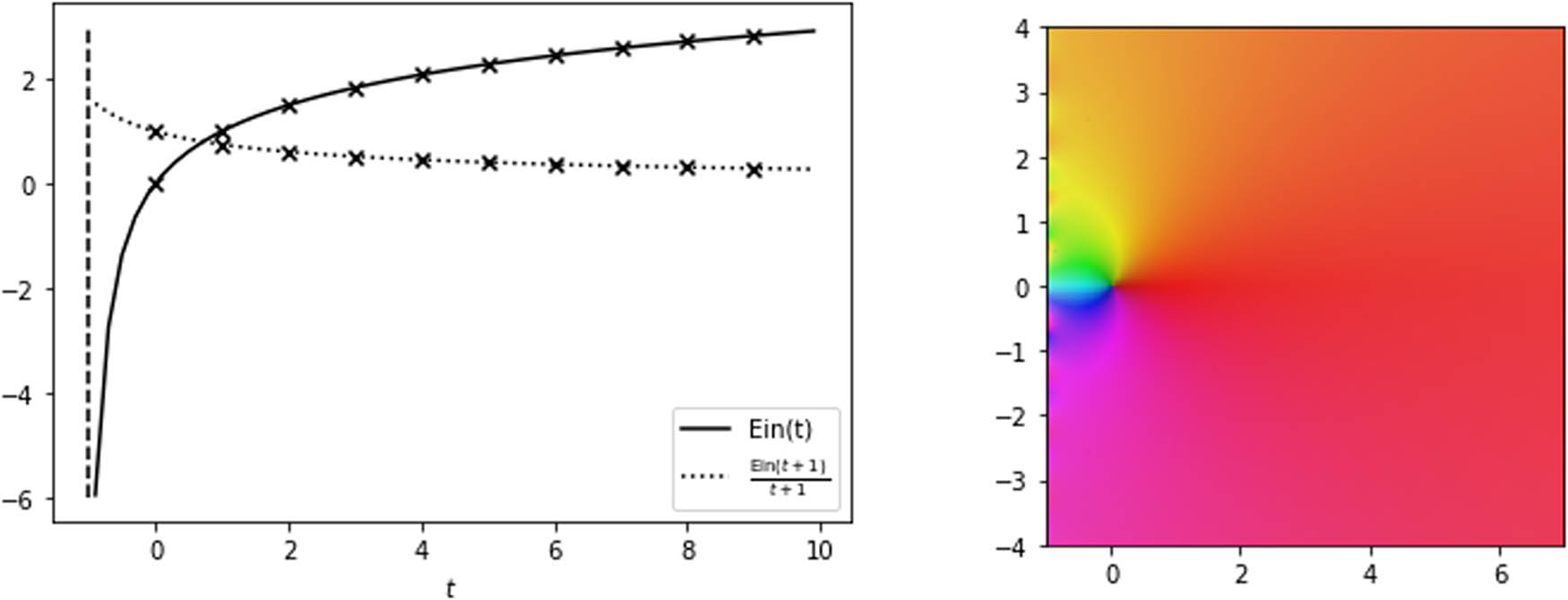
Plot of both
Theorem 4.6
The following formula holds:
Proof
Using (5), calculate
which completes the proof.□
5 Conclusion
We have introduced the discrete analogues of the sine integral and complementary exponential integral functions. For each, we have expressed it as a series, found its relationship to hypergeometric functions, and computed its Laplace transform. Analytic continuation is likely a way to extend the domains of existence of
We have argued in Remark 4.1 that an integral form for
There are other related functions that were not considered here, of most importance would be analogues of the exponential integrals
Acknowledgements
The authors thank Treston Brown for participating in undergraduate research in 2017 under Tom Cuchta, initiating the study of the discrete sine integral.
-
Conflict of interest: The authors claim no conflict of interest.
References
[1] J. M. Davis, I. A. Gravagne, B. J. Jackson, R. J. Marks II, and A. A. Ramos, The Laplace transform on time scales revisited, J. Math. Anal. Appl. 332 (2007), no. 2, 1291–1307. 10.1016/j.jmaa.2006.10.089Search in Google Scholar
[2] B. J. Jackson, A general linear systems theory on time scales: transforms, stability, and control, Baylor University, Waco, Texas, 2007. Search in Google Scholar
[3] M. Bohner and T. Cuchta, The Bessel difference equation, Proc. Amer. Math. Soc. 145 (2017), no. 4, 1567–1580. 10.1090/proc/13416Search in Google Scholar
[4] A. Slavík, Discrete Bessel functions and partial difference equations, J. Difference Equ. Appl. 24 (2018), no. 3, 425–437. 10.1080/10236198.2017.1416107Search in Google Scholar
[5] M. Bohner and T. Cuchta, The generalized hypergeometric difference equation, Demonstr. Math. 51 (2018), no. 1, 62–75. 10.1515/dema-2018-0007Search in Google Scholar
[6] T. Cuchta, D. Grow, and Nick Wintz, Discrete matrix hypergeometric functions, J. Math. Anal. Appl. 518 (2023), no. 2, Paper No. 126716, 14. 10.1016/j.jmaa.2022.126716Search in Google Scholar
[7] G. A. Monteiro and A. SlavÍk, Generalized elementary functions, J. Math. Anal. Appl. 411 (2014), no. 2, 838–852. 10.1016/j.jmaa.2013.10.010Search in Google Scholar
[8] M. Bohner and A. Peterson, Dynamic Equations on Time Scales, Birkhäuser Boston, Inc., Boston, MA, 2001, An introduction with applications. 10.1007/978-1-4612-0201-1Search in Google Scholar
[9] M. Bohner, G. S. Guseinov, and B. Karpuz, Properties of the Laplace transform on time scales with arbitrary graininess, Integral Transforms Spec. Funct. 22 (2011), no. 11, 785–800. 10.1080/10652469.2010.548335Search in Google Scholar
[10] M. Bohner, G. S. Guseinov, and B. Karpuz, Further properties of the Laplace transform on time scales with arbitrary graininess, Integral Transforms Special Funct. 24 (2013), no. 4, 289–301. 10.1080/10652469.2012.689300Search in Google Scholar
[11] A. P. Prudnikov and O. I. Marichev, Integrals and Series: Direct Laplace Transforms, vol. 4, CRC Press, Boca Raton, Florida, USA, 1992. Search in Google Scholar
[12] K. Oldham, J. Myland, and J. Spanier, An atlas of functions, 2nd ed., Springer, New York, 2009, With Equator, the atlas function calculator, With 1 CD-ROM (Windows). 10.1007/978-0-387-48807-3Search in Google Scholar
[13] F. Mainardi and E. Masina, On modifications of the exponential integral with the Mittag-Leffler function, Fract. Calc. Appl. Anal. 21 (2018), no. 5, 1156–1169. 10.1515/fca-2018-0063Search in Google Scholar
[14] R. J. Marks II, I. A. Gravagne, J. M. Davis, and J. J. DaCunha, Nonregressivity in switched linear circuits and mechanical systems, Math. Comput. Modell. 43 (2006), no. 11–12, 1383–1392. 10.1016/j.mcm.2005.08.007Search in Google Scholar
[15] M. Bohner and G. S. Guseinov, An introduction to complex functions on products of two time scales, J. Difference Equations Appl. 12 (2006), no. 3–4, 369–384. 10.1080/10236190500489657Search in Google Scholar
[16] S. Smirnov, Discrete complex analysis and probability, Proceedings of the International Congress of Mathematicians, Vol. I, Hindustan Book Agency, New Delhi, 2010, pp. 595–621. 10.1142/9789814324359_0026Search in Google Scholar
[17] L. Lovász, Discrete analytic functions: an exposition, Surveys in Differential Geometry, vol. 9, Int. Press, Somerville, MA, 2004, pp. 241–273. 10.4310/SDG.2004.v9.n1.a7Search in Google Scholar
© 2023 the author(s), published by De Gruyter
This work is licensed under the Creative Commons Attribution 4.0 International License.
Articles in the same Issue
- Regular Articles
- A novel class of bipolar soft separation axioms concerning crisp points
- Duality for convolution on subclasses of analytic functions and weighted integral operators
- Existence of a solution to an infinite system of weighted fractional integral equations of a function with respect to another function via a measure of noncompactness
- On the existence of nonnegative radial solutions for Dirichlet exterior problems on the Heisenberg group
- Hyers-Ulam stability of isometries on bounded domains-II
- Asymptotic study of Leray solution of 3D-Navier-Stokes equations with exponential damping
- Semi-Hyers-Ulam-Rassias stability for an integro-differential equation of order 𝓃
- Jordan triple (α,β)-higher ∗-derivations on semiprime rings
- The asymptotic behaviors of solutions for higher-order (m1, m2)-coupled Kirchhoff models with nonlinear strong damping
- Approximation of the image of the Lp ball under Hilbert-Schmidt integral operator
- Best proximity points in ℱ-metric spaces with applications
- Approximation spaces inspired by subset rough neighborhoods with applications
- A numerical Haar wavelet-finite difference hybrid method and its convergence for nonlinear hyperbolic partial differential equation
- A novel conservative numerical approximation scheme for the Rosenau-Kawahara equation
- Fekete-Szegö functional for a class of non-Bazilevic functions related to quasi-subordination
-
On local fractional integral inequalities via generalized
- On some geometric results for generalized k-Bessel functions
- Convergence analysis of M-iteration for 𝒢-nonexpansive mappings with directed graphs applicable in image deblurring and signal recovering problems
- Some results of homogeneous expansions for a class of biholomorphic mappings defined on a Reinhardt domain in ℂn
- Graded weakly 1-absorbing primary ideals
- The existence and uniqueness of solutions to a functional equation arising in psychological learning theory
- Some aspects of the n-ary orthogonal and b(αn,βn)-best approximations of b(αn,βn)-hypermetric spaces over Banach algebras
- Numerical solution of a malignant invasion model using some finite difference methods
- Increasing property and logarithmic convexity of functions involving Dirichlet lambda function
- Feature fusion-based text information mining method for natural scenes
- Global optimum solutions for a system of (k, ψ)-Hilfer fractional differential equations: Best proximity point approach
- The study of solutions for several systems of PDDEs with two complex variables
- Regularity criteria via horizontal component of velocity for the Boussinesq equations in anisotropic Lorentz spaces
- Generalized Stević-Sharma operators from the minimal Möbius invariant space into Bloch-type spaces
- On initial value problem for elliptic equation on the plane under Caputo derivative
- A dimension expanded preconditioning technique for block two-by-two linear equations
- Asymptotic behavior of Fréchet functional equation and some characterizations of inner product spaces
- Small perturbations of critical nonlocal equations with variable exponents
- Dynamical property of hyperspace on uniform space
- Some notes on graded weakly 1-absorbing primary ideals
- On the problem of detecting source points acting on a fluid
- Integral transforms involving a generalized k-Bessel function
- Ruled real hypersurfaces in the complex hyperbolic quadric
- On the monotonic properties and oscillatory behavior of solutions of neutral differential equations
- Approximate multi-variable bi-Jensen-type mappings
- Mixed-type SP-iteration for asymptotically nonexpansive mappings in hyperbolic spaces
- On the equation fn + (f″)m ≡ 1
- Results on the modified degenerate Laplace-type integral associated with applications involving fractional kinetic equations
- Characterizations of entire solutions for the system of Fermat-type binomial and trinomial shift equations in ℂn#
- Commentary
- On I. Meghea and C. S. Stamin review article “Remarks on some variants of minimal point theorem and Ekeland variational principle with applications,” Demonstratio Mathematica 2022; 55: 354–379
- Special Issue on Fixed Point Theory and Applications to Various Differential/Integral Equations - Part II
- On Cauchy problem for pseudo-parabolic equation with Caputo-Fabrizio operator
- Fixed-point results for convex orbital operators
- Asymptotic stability of equilibria for difference equations via fixed points of enriched Prešić operators
- Asymptotic behavior of resolvents of equilibrium problems on complete geodesic spaces
- A system of additive functional equations in complex Banach algebras
- New inertial forward–backward algorithm for convex minimization with applications
- Uniqueness of solutions for a ψ-Hilfer fractional integral boundary value problem with the p-Laplacian operator
- Analysis of Cauchy problem with fractal-fractional differential operators
- Common best proximity points for a pair of mappings with certain dominating property
- Investigation of hybrid fractional q-integro-difference equations supplemented with nonlocal q-integral boundary conditions
- The structure of fuzzy fractals generated by an orbital fuzzy iterated function system
- On the structure of self-affine Jordan arcs in ℝ2
- Solvability for a system of Hadamard-type hybrid fractional differential inclusions
- Three solutions for discrete anisotropic Kirchhoff-type problems
- On split generalized equilibrium problem with multiple output sets and common fixed points problem
- Special Issue on Computational and Numerical Methods for Special Functions - Part II
- Sandwich-type results regarding Riemann-Liouville fractional integral of q-hypergeometric function
- Certain aspects of Nörlund ℐ-statistical convergence of sequences in neutrosophic normed spaces
- On completeness of weak eigenfunctions for multi-interval Sturm-Liouville equations with boundary-interface conditions
- Some identities on generalized harmonic numbers and generalized harmonic functions
- Study of degenerate derangement polynomials by λ-umbral calculus
- Normal ordering associated with λ-Stirling numbers in λ-shift algebra
- Analytical and numerical analysis of damped harmonic oscillator model with nonlocal operators
- Compositions of positive integers with 2s and 3s
- Kinematic-geometry of a line trajectory and the invariants of the axodes
- Hahn Laplace transform and its applications
- Discrete complementary exponential and sine integral functions
- Special Issue on Recent Methods in Approximation Theory - Part II
- On the order of approximation by modified summation-integral-type operators based on two parameters
- Bernstein-type operators on elliptic domain and their interpolation properties
- A class of strongly convergent subgradient extragradient methods for solving quasimonotone variational inequalities
- Special Issue on Recent Advances in Fractional Calculus and Nonlinear Fractional Evaluation Equations - Part II
- Application of fractional quantum calculus on coupled hybrid differential systems within the sequential Caputo fractional q-derivatives
- On some conformable boundary value problems in the setting of a new generalized conformable fractional derivative
- A certain class of fractional difference equations with damping: Oscillatory properties
- Weighted Hermite-Hadamard inequalities for r-times differentiable preinvex functions for k-fractional integrals
- Special Issue on Recent Advances for Computational and Mathematical Methods in Scientific Problems - Part II
- The behavior of hidden bifurcation in 2D scroll via saturated function series controlled by a coefficient harmonic linearization method
- Phase portraits of two classes of quadratic differential systems exhibiting as solutions two cubic algebraic curves
- Petri net analysis of a queueing inventory system with orbital search by the server
- Asymptotic stability of an epidemiological fractional reaction-diffusion model
- On the stability of a strongly stabilizing control for degenerate systems in Hilbert spaces
- Special Issue on Application of Fractional Calculus: Mathematical Modeling and Control - Part I
- New conticrete inequalities of the Hermite-Hadamard-Jensen-Mercer type in terms of generalized conformable fractional operators via majorization
- Pell-Lucas polynomials for numerical treatment of the nonlinear fractional-order Duffing equation
- Impacts of Brownian motion and fractional derivative on the solutions of the stochastic fractional Davey-Stewartson equations
- Some results on fractional Hahn difference boundary value problems
- Properties of a subclass of analytic functions defined by Riemann-Liouville fractional integral applied to convolution product of multiplier transformation and Ruscheweyh derivative
- Special Issue on Development of Fuzzy Sets and Their Extensions - Part I
- The cross-border e-commerce platform selection based on the probabilistic dual hesitant fuzzy generalized dice similarity measures
- Comparison of fuzzy and crisp decision matrices: An evaluation on PROBID and sPROBID multi-criteria decision-making methods
- Rejection and symmetric difference of bipolar picture fuzzy graph