The behavior of hidden bifurcation in 2D scroll via saturated function series controlled by a coefficient harmonic linearization method
-
Zaamoune Faiza
 and
Menacer Tidjani
and
Menacer Tidjani

Abstract
In this article, the behavior of hidden bifurcation in a two-dimensional (2D) scroll via saturated function series controlled by the coefficient harmonic linearization method is presented. A saturated function series approach for chaos generation. The systematic saturated function series methodicalness improved here can make multi-scroll and grid scroll chaotic attractors from a 3D linear autonomous system with a plain saturated function series supervisor. We have used a hidden bifurcation method in grid scroll., where the method of hidden bifurcation presented by Menacer, et al. in (2016) for Chua multi-scroll attractors. This additional parameter, which is absent from the initial problem, is perfectly adapted to unfold the structure of the multispiral chaotic attractor. The novelty of this article is twofold: first, the saturated function series model for hidden bifurcation in a 2 – D scroll; and second, the control of hidden bifurcation behavior by the value of the harmonic coefficient
1 Introduction
During precedent and until now, the generation of multispiral chaotic attractors has been extensively examined due to their hopeful applications in manifold real-world technologies. Few techniques have been suggested, like linear and nonlinear modulating functions and in electronic circuits (saturated circuits, etc.), for generating multispiral chaotic attractors see [1–3]. The issue of hidden oscillations in nonlinear control systems forces us to improvise a novel approximation of nonlinear oscillation theory. Meanwhile, during the initial institution and evolution of the theory of nonlinear oscillations in the first half of the twentieth century broad attention was given to the analysis and composite of oscillating systems, for which the solution of existing problems of oscillating ranks was not too uneasy [4].
The construction itself of many systems was such that they had oscillating solutions, the nature of which was almost clear. The rise in these systems’ periodic solutions was visible by numerical analysis when the numerical integration procedure of the trajectories permitted one to track from the little neighborhood of equilibrium to a periodic trajectory [5,6]. A self-excited attractor’s basin of attraction interferes with the neighborhood of an equilibrium point, whereas a hidden attractor’s basin of attraction does not intersect with the small neighborhoods of any equilibrium points, making it hard to find. The hidden attractors are important in engineering applications [1,7–15]. Though most multi-spirals generations are have been known for many years, it is only recently that they have been studied underneath the area of bifurcation theory [14]. In all the multispirals previously familiar, the number of spirals (or scrolls) is a fixed integer, whereas it depends on one or more discrete parameters after the rapid development in more than a decade. In [14], the authors modified the model of discrete parameters by producing hidden bifurcations and generating multispirals.
Thus, hidden bifurcation theory is instituted based on the hidden attractor theory introduced by Leonov et al. [8,10]. In this work, the focus is on the study of paradigm hidden bifurcation in 2D grid scroll chaotic attractors generated by saturated function series. In the work of Chen et al., a saturated function series was suggested for generating multispiral chaotic attractors, including 1D
The aspects of this article are as follows: (i) the study of hidden bifurcation of 2D
This article is organized as follows: in Section 2, we first present the model of 2D
2 Analytical-numerical method for double-spiral chaotic attractors from saturated function series
2.1 Double-spiral attractors generated via a saturated function series
In the following, to create a 2D
where
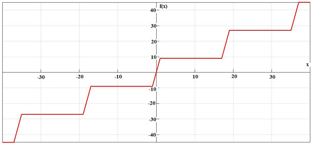
Graph of saturated function series for
The parameters
So, the number
For

Two-directional
2.1.1 Attraction basin of the nine spirals attractors
For our system (1-2-3), we have a
For all equilibria in two sets
In this obstacle, we took

The attraction basin of 9 spirals attractors. (a) Attraction basin attractors cross section passing through four equilibrium points
2.2 Analytical-numerical method for attractors localization
Twelve years ago, Leonov [10], Leonov and Kuznetsov [11,13], proposed an effective method for the numerical localization of hidden attractors in multidimensional dynamical systems. They improve this method, especially for Chua attractors. In 2016, the method developed by Menacer et al. to discover hidden bifurcations in the multispiral Chua attractor was published. For the search of periodic solution close to harmonic oscillation, we consider a coefficient of harmonic linearization
where
which
where
Suppose that the function
and determine a stable nontrivial periodic solution
So
2.3 Poincare map for harmonic linearization in vector case
Define system (8) with
is satisfied. In a phase space of system (8), we introduce the following formula:
Hither,
By using the conditions (10) and (8) for the solutions with initial data from
From relation (13), it follows that for any point
such as relations
are not verified. Construct a Poincare map
Introduce the describing function
From relation (13) and condition (10) for solutions of system (8), we obtain the following relations:
Theorem 1
If the inequalities
are verified, then, for
From this theorem, and the Brouwer fixed point theorem, we have the following conclusions.
Theorem 2
If the inequalities (20) are verified, then, for
This solution is stable in the sense that its neighborhood
Theorem 3
If the conditions
are verified, then for
2.3.1 Justification of hidden bifurcation in a 2D scroll via saturated function series (harmonic linearization method in vector case)
The Theorems 1–3 were proved that the positive parameter
The previous work [16] has proven a hidden bifurcation in multispirals generated by saturated function series, which is similar to the method introduced by Menacer et al. [14] for Chua multi-scroll attractors. In this work, we apply the above-described multi-step procedure for the localization of hidden bifurcation in vector case (Poincare map harmonic linearization), and we developed for study a hidden bifurcation in 2D scroll.
After a lot of calculation for our system (1–3), we found a field for the parameter
in this field, we noted that the last three theorems are satisfied. For our system, we took
3 Method for uncovering hidden bifurcations (2D scroll)
Theorem 2 can be used for looking hidden bifurcation with
Here,
Define the coefficient
where
The transfer function
From this transfer function
3.1 Numerical result of hidden bifurcation in 2D scroll
The goal of this article is to study the hidden bifurcation in a 2D scroll, and we focused on the behavior of spirals when we took one value for coefficient harmonic linearization and two values for coefficient harmonic linearization for the solutions of system 26.
3.1.1 One value for coefficient harmonic linearization
In the first, we took one value for the coefficient of harmonic linearization
and for
Using these initial data, the procedure described above in Section 2 produces the values of the parameter
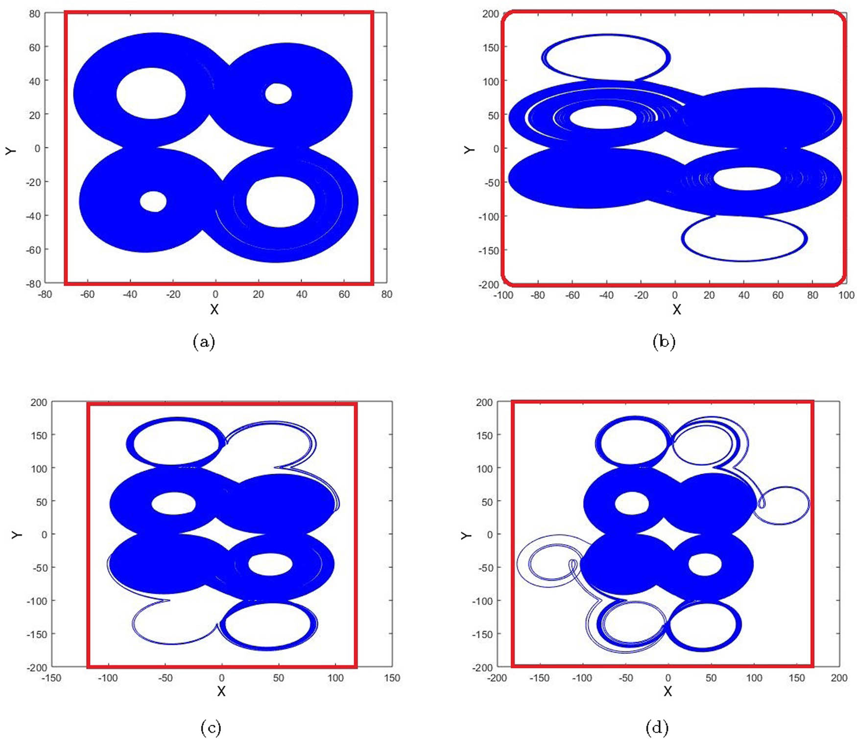
Numerical results of 2D hidden bifurcations for
| Values of
|
0.55 | 0.7 | 0.75 | 0.82 | 0.85 | 0.93 |
| Number of spirals | 2 | 4 | 5 | 7 | 8 | 9 |


Remark 1
In the case
Numerical results of 2D hidden bifurcations for
| Values of
|
0.55 | 0.7 | 0.8 | 0.829 |
| Number of spirals | 2 | 4 | 6 | 8 |
| Values of
|
0.83 | 0.86 | 0.865 | 0.94 |
| Number of spirals | 10 | 12 | 14 | 16 |
Remark 2
In the case

The increasing number of spirals of system (1-2-3) according to increasing
3.1.2 Two values for coefficient harmonic linearization
We took two values of the coefficient of harmonic linearization
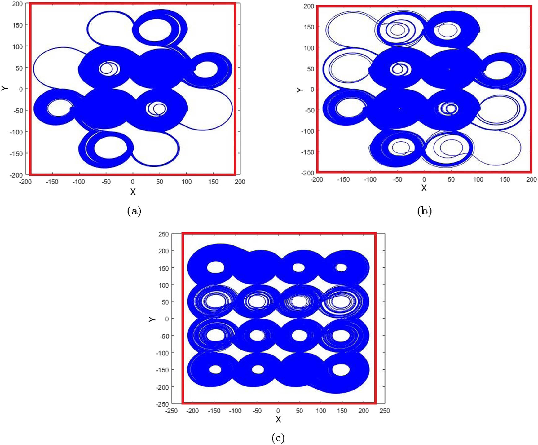
The results about the behavior of points bifurcations each spiral genesis in the cell (oblong) and the appearance of points bifurcation organized two-by-two-in all number of the scroll. For this purpose, we studied a 16 scroll for
Numerical results of 2D hidden bifurcations for
| Values of
|
0.55 | 0.85 | 0.867 | 0.873 | 0.9 | 0.915 | 1 |
| Number of spirals | 4 | 6 | 8 | 10 | 12 | 14 | 16 |
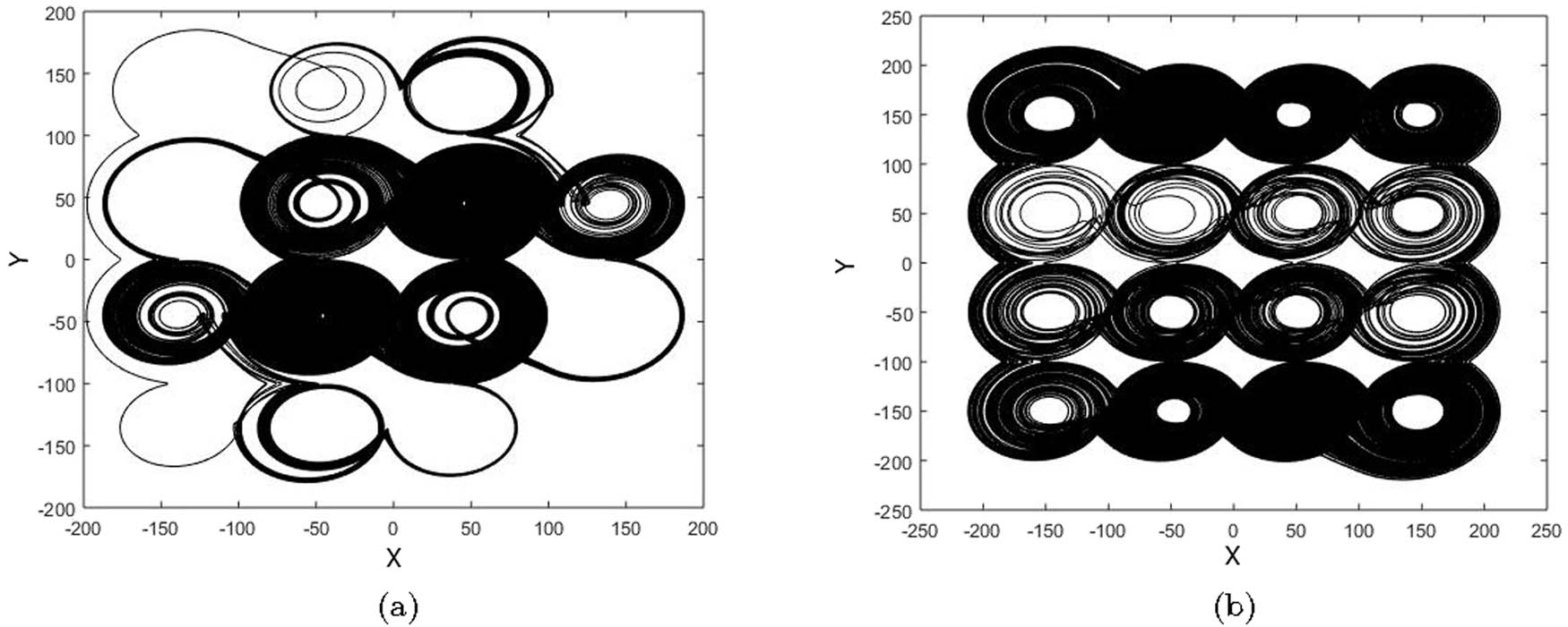
The increasing number of spirals of system (1-2-3) according to the increasing
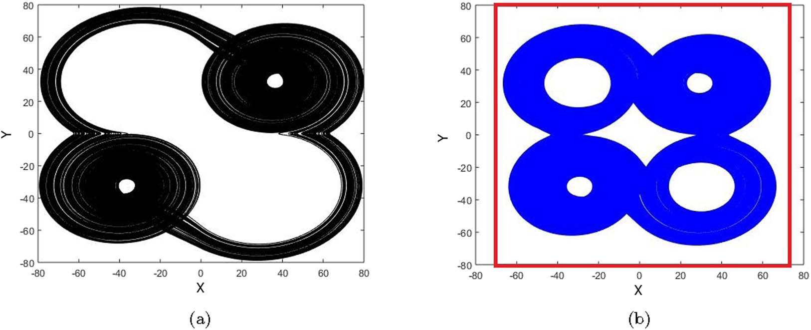
The comparison between the behavior of spirals of system (1-2-3) according to increasing
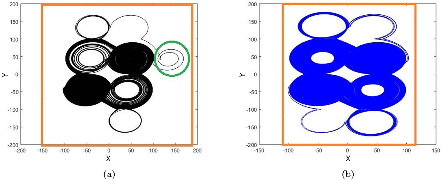
The comparison between the behavior of spirals of system (1-2-3) according to increasing
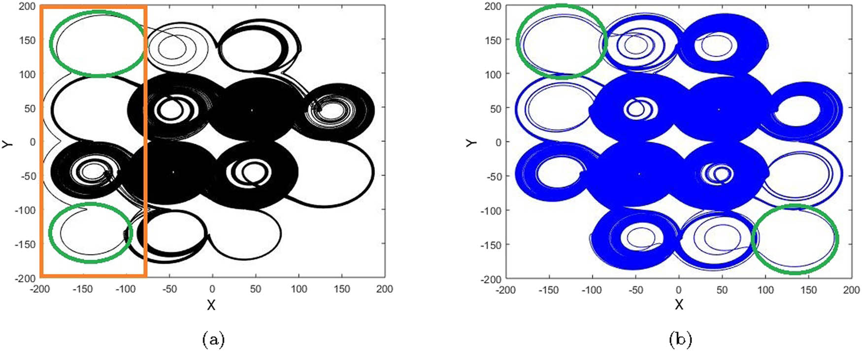
The comparison between the behavior of spirals of system (1-2-3) according to increasing
Remark 3
In our results, we noted that the coefficient harmonic linearization controlled the apparition behavior of hidden bifurcation, and in the case of two values for the coefficient harmonic linearization, we noted that it organized the apparition behavior of the hidden bifurcation better than the first case.
4 Conclusion
This article has initiated the behavior of hidden bifurcation in scroll via a saturated function series controlled by the coefficient harmonic linearization method, where a saturated function series approach is used for generating multi-scroll chaotic attractors, including 1D-scroll, 2D-grid scroll, and 3D-grid scroll attractors [9] from a given 1D-2D linear autonomic system with a saturated function series as the controller. In particular, a 2D Poincaré return map has been harshly structured to fulfill the chaotic behaviors of the double-scroll attractor. The method used is similar to the one presented by Leonov [10] and Leonov and Kuznetsov [11]. Such hidden bifurcations were first uncovered in 2016 for Chua multi-scroll attractors, which depend on a discrete parameter [14]. The novelties that this article introduces are (i) the model hidden bifurcation in a 2D scroll via saturated function series and (ii) controlling the behavior of a hidden bifurcation by the value of coefficient harmonic
-
Funding information: The authors state that there is no funding involved.
-
Author contributions: Zaamoune Faiza developed the code Matlab and simulations and wrote the article. Menacer Tidjani designed the experiments and corrected grammatical and stylistic errors.
-
Conflict of interest: The authors state no conflict of interest.
-
Informed consent: Informed consent has been obtained from all individuals included in this study.
-
Ethical approval: The conducted research is not related to either human or animals use.
-
Data availability statement: The datasets generated and/or analyzed during the current study are available from the corresponding author on reasonable request.
References
[1] J. Lü and G. Chen, Generating multiscroll chaotic attractors: Theories, methods and applications, Int J Bifurcat Chaos 16 (2006), no. 4, 775–858, DOI: https://doi.org/10.1142/S0218127406015179. 10.1142/S0218127406015179Search in Google Scholar
[2] X. Zhang and Ch. Wang, A novel multi-attractor period multi-scroll chaotic integrated circuit based on CMOS wide adjustable CCCII, IEEE Access 7 (2019), no. 1, 16336–16350, DOI: https://doi.org/10.1109/ACCESS.2019.2894853. 10.1109/ACCESS.2019.2894853Search in Google Scholar
[3] H. Lin, Ch. Wang, Y. Sun, and T. Wang, Generating n-scroll chaotic attractors from a memristor-based magnetized hopfield neural network, IEEE Trans. Circuits Syst II Express Briefs 70 (2023), no. 1, 311–315, DOI: https://doi.org/10.1109/TCSII.2022.3212394. 10.1109/TCSII.2022.3212394Search in Google Scholar
[4] H. Lin, Ch. Wang, C. Xu, and X. Zhang, A memristive synapse control method to generate diversified multi-structure chaotic attractors, IEEE Trans Computer-aided Design Integrated Circuits Syst. 42 (2022), no. 3, 942–955, DOI: https://doi.org/10.1109/TCSII.2022.3186516. 10.1109/TCAD.2022.3186516Search in Google Scholar
[5] L. Zhou, Ch. Wang, and L. Zhou, Generating hyperchaotic multi-wing attractor in a 4D memristive circuit, Nonlinear Dyn. 85 (2016), no. 4, 2653–2663, DOI: http://dx.doi.org/10.10072Fs11071-016-2852-8. 10.1007/s11071-016-2852-8Search in Google Scholar
[6] L. Zhou, Ch. Wang, and L. Zhou, A novel no-equilibrium hyperchaotic multi-wing system via introducing memristor, Int. J. Circuit Theory Appl. 46 (2018), no. 1, 84–98, DOI: https://doi.org/10.1002/cta.2339. 10.1002/cta.2339Search in Google Scholar
[7] Q. Deng and C. Wang, Multi-scroll hidden attractors with two stable equilibrium points, Chaos 29 (2019), no. 9, 093112, DOI: https://doi.org/10.1063/1.5116732. 10.1063/1.5116732Search in Google Scholar PubMed
[8] G. A. Leonov, N. V. Kuznetsov, and V. I. Vagaitsev, Hidden attractor in smooth Chua systems, Physica D 241 (2012), no. 18, 1482–1486, DOI: https://doi.org/10.1016/j.physd.2012.05.016. 10.1016/j.physd.2012.05.016Search in Google Scholar
[9] J. Lü, G. Chen, X. Yu, and H. Leung, Design and analysis of multiscroll chaotic attractors from saturated function series, IEEE Trans. Circuits Syst. 51 (2004), no. 12, 2476–2490, DOI: https://doi.org/10.1109/TCSI.2004.838151. 10.1109/TCSI.2004.838151Search in Google Scholar
[10] G. A. Leonov, Effective methods for periodic oscillations search in dynamical systems, Appl. Math. Mech. 74 (2010), no. 1, 37–73, DOI: http://dx.doi.org/10.1016/j.jappmathmech.2010.03.004. 10.1016/j.jappmathmech.2010.03.004Search in Google Scholar
[11] G. A. Leonov and N. V. Kuznetsov, Localization of hidden Chua’s attractors, Phys. Lett. A 375 (2011), no. 23, 2230–2233, DOI: https://doi.org/10.1016/j.physleta.2011.04.037. 10.1016/j.physleta.2011.04.037Search in Google Scholar
[12] G. A. Leonov and N. V. Kuznetsov, Analytical numerical methods for investigation of hidden oscillations in nonlinear control systems, Proc. 18th IFAC World Congress, Milano, Italy 18 (2011), no. 1, 2494–2505, DOI: http://dx.doi.org/10.3182/20110828-6-IT-1002.03315. 10.3182/20110828-6-IT-1002.03315Search in Google Scholar
[13] G. A. Leonov and N. V. Kuznetsov, Hidden attractors in dynamical systems. From hidden oscillations in Hilbert-Kolmogrov, Aizerman, and Kalman problems to hidden chaotic attractor in Chua circuits, Int. J. Bifurcat. Chaos 23 (2013), no. 1, 1330002–13300071, DOI: https://doi.org/10.1142/S0218127413300024. 10.1142/S0218127413300024Search in Google Scholar
[14] T. Menacer, R. Lozi, and L. O. Chua, Hidden bifurcations in the multispiral Chua attractor, Int. J. Bifurcat. Chaos 16 (2016), no. 4, 1630039–1630065, DOI: https://dx.doi.org/10.1142/S0218127416300391. 10.1142/S0218127416300391Search in Google Scholar
[15] X. Zhang and C. Wang, Multiscroll hyperchaotic system with hidden attractors and its circuit implementation, Int. J. Bifurcat. Chaos 29 (2019), no. 9, 1950117, DOI: https://doi.org/10.1142/S0218127419501177. 10.1142/S0218127419501177Search in Google Scholar
[16] F. Zaamoune, T. Menacer, R. Lozi, and G. Chen, Symmetries in hidden bifurcation routes to multiscroll chaotic attractors generated by saturated function series, J. Adv. Eng. Comput. 3 (2019), no. 4, 511–522, DOI: https://doi.org/10.1142/S0218127419501177. 10.25073/jaec.201934.256Search in Google Scholar
© 2023 the author(s), published by De Gruyter
This work is licensed under the Creative Commons Attribution 4.0 International License.
Articles in the same Issue
- Regular Articles
- A novel class of bipolar soft separation axioms concerning crisp points
- Duality for convolution on subclasses of analytic functions and weighted integral operators
- Existence of a solution to an infinite system of weighted fractional integral equations of a function with respect to another function via a measure of noncompactness
- On the existence of nonnegative radial solutions for Dirichlet exterior problems on the Heisenberg group
- Hyers-Ulam stability of isometries on bounded domains-II
- Asymptotic study of Leray solution of 3D-Navier-Stokes equations with exponential damping
- Semi-Hyers-Ulam-Rassias stability for an integro-differential equation of order 𝓃
- Jordan triple (α,β)-higher ∗-derivations on semiprime rings
- The asymptotic behaviors of solutions for higher-order (m1, m2)-coupled Kirchhoff models with nonlinear strong damping
- Approximation of the image of the Lp ball under Hilbert-Schmidt integral operator
- Best proximity points in ℱ-metric spaces with applications
- Approximation spaces inspired by subset rough neighborhoods with applications
- A numerical Haar wavelet-finite difference hybrid method and its convergence for nonlinear hyperbolic partial differential equation
- A novel conservative numerical approximation scheme for the Rosenau-Kawahara equation
- Fekete-Szegö functional for a class of non-Bazilevic functions related to quasi-subordination
-
On local fractional integral inequalities via generalized
- On some geometric results for generalized k-Bessel functions
- Convergence analysis of M-iteration for 𝒢-nonexpansive mappings with directed graphs applicable in image deblurring and signal recovering problems
- Some results of homogeneous expansions for a class of biholomorphic mappings defined on a Reinhardt domain in ℂn
- Graded weakly 1-absorbing primary ideals
- The existence and uniqueness of solutions to a functional equation arising in psychological learning theory
- Some aspects of the n-ary orthogonal and b(αn,βn)-best approximations of b(αn,βn)-hypermetric spaces over Banach algebras
- Numerical solution of a malignant invasion model using some finite difference methods
- Increasing property and logarithmic convexity of functions involving Dirichlet lambda function
- Feature fusion-based text information mining method for natural scenes
- Global optimum solutions for a system of (k, ψ)-Hilfer fractional differential equations: Best proximity point approach
- The study of solutions for several systems of PDDEs with two complex variables
- Regularity criteria via horizontal component of velocity for the Boussinesq equations in anisotropic Lorentz spaces
- Generalized Stević-Sharma operators from the minimal Möbius invariant space into Bloch-type spaces
- On initial value problem for elliptic equation on the plane under Caputo derivative
- A dimension expanded preconditioning technique for block two-by-two linear equations
- Asymptotic behavior of Fréchet functional equation and some characterizations of inner product spaces
- Small perturbations of critical nonlocal equations with variable exponents
- Dynamical property of hyperspace on uniform space
- Some notes on graded weakly 1-absorbing primary ideals
- On the problem of detecting source points acting on a fluid
- Integral transforms involving a generalized k-Bessel function
- Ruled real hypersurfaces in the complex hyperbolic quadric
- On the monotonic properties and oscillatory behavior of solutions of neutral differential equations
- Approximate multi-variable bi-Jensen-type mappings
- Mixed-type SP-iteration for asymptotically nonexpansive mappings in hyperbolic spaces
- On the equation fn + (f″)m ≡ 1
- Results on the modified degenerate Laplace-type integral associated with applications involving fractional kinetic equations
- Characterizations of entire solutions for the system of Fermat-type binomial and trinomial shift equations in ℂn#
- Commentary
- On I. Meghea and C. S. Stamin review article “Remarks on some variants of minimal point theorem and Ekeland variational principle with applications,” Demonstratio Mathematica 2022; 55: 354–379
- Special Issue on Fixed Point Theory and Applications to Various Differential/Integral Equations - Part II
- On Cauchy problem for pseudo-parabolic equation with Caputo-Fabrizio operator
- Fixed-point results for convex orbital operators
- Asymptotic stability of equilibria for difference equations via fixed points of enriched Prešić operators
- Asymptotic behavior of resolvents of equilibrium problems on complete geodesic spaces
- A system of additive functional equations in complex Banach algebras
- New inertial forward–backward algorithm for convex minimization with applications
- Uniqueness of solutions for a ψ-Hilfer fractional integral boundary value problem with the p-Laplacian operator
- Analysis of Cauchy problem with fractal-fractional differential operators
- Common best proximity points for a pair of mappings with certain dominating property
- Investigation of hybrid fractional q-integro-difference equations supplemented with nonlocal q-integral boundary conditions
- The structure of fuzzy fractals generated by an orbital fuzzy iterated function system
- On the structure of self-affine Jordan arcs in ℝ2
- Solvability for a system of Hadamard-type hybrid fractional differential inclusions
- Three solutions for discrete anisotropic Kirchhoff-type problems
- On split generalized equilibrium problem with multiple output sets and common fixed points problem
- Special Issue on Computational and Numerical Methods for Special Functions - Part II
- Sandwich-type results regarding Riemann-Liouville fractional integral of q-hypergeometric function
- Certain aspects of Nörlund ℐ-statistical convergence of sequences in neutrosophic normed spaces
- On completeness of weak eigenfunctions for multi-interval Sturm-Liouville equations with boundary-interface conditions
- Some identities on generalized harmonic numbers and generalized harmonic functions
- Study of degenerate derangement polynomials by λ-umbral calculus
- Normal ordering associated with λ-Stirling numbers in λ-shift algebra
- Analytical and numerical analysis of damped harmonic oscillator model with nonlocal operators
- Compositions of positive integers with 2s and 3s
- Kinematic-geometry of a line trajectory and the invariants of the axodes
- Hahn Laplace transform and its applications
- Discrete complementary exponential and sine integral functions
- Special Issue on Recent Methods in Approximation Theory - Part II
- On the order of approximation by modified summation-integral-type operators based on two parameters
- Bernstein-type operators on elliptic domain and their interpolation properties
- A class of strongly convergent subgradient extragradient methods for solving quasimonotone variational inequalities
- Special Issue on Recent Advances in Fractional Calculus and Nonlinear Fractional Evaluation Equations - Part II
- Application of fractional quantum calculus on coupled hybrid differential systems within the sequential Caputo fractional q-derivatives
- On some conformable boundary value problems in the setting of a new generalized conformable fractional derivative
- A certain class of fractional difference equations with damping: Oscillatory properties
- Weighted Hermite-Hadamard inequalities for r-times differentiable preinvex functions for k-fractional integrals
- Special Issue on Recent Advances for Computational and Mathematical Methods in Scientific Problems - Part II
- The behavior of hidden bifurcation in 2D scroll via saturated function series controlled by a coefficient harmonic linearization method
- Phase portraits of two classes of quadratic differential systems exhibiting as solutions two cubic algebraic curves
- Petri net analysis of a queueing inventory system with orbital search by the server
- Asymptotic stability of an epidemiological fractional reaction-diffusion model
- On the stability of a strongly stabilizing control for degenerate systems in Hilbert spaces
- Special Issue on Application of Fractional Calculus: Mathematical Modeling and Control - Part I
- New conticrete inequalities of the Hermite-Hadamard-Jensen-Mercer type in terms of generalized conformable fractional operators via majorization
- Pell-Lucas polynomials for numerical treatment of the nonlinear fractional-order Duffing equation
- Impacts of Brownian motion and fractional derivative on the solutions of the stochastic fractional Davey-Stewartson equations
- Some results on fractional Hahn difference boundary value problems
- Properties of a subclass of analytic functions defined by Riemann-Liouville fractional integral applied to convolution product of multiplier transformation and Ruscheweyh derivative
- Special Issue on Development of Fuzzy Sets and Their Extensions - Part I
- The cross-border e-commerce platform selection based on the probabilistic dual hesitant fuzzy generalized dice similarity measures
- Comparison of fuzzy and crisp decision matrices: An evaluation on PROBID and sPROBID multi-criteria decision-making methods
- Rejection and symmetric difference of bipolar picture fuzzy graph