Comparison of fuzzy and crisp decision matrices: An evaluation on PROBID and sPROBID multi-criteria decision-making methods
-
Zhiyuan Wang
 ,
Željko Stević
,
Abdullah Özçil
,
Željko Stević
,
Abdullah Özçil

Abstract
The use of multi-criteria decision-making (MCDM) methods to select the most appropriate one from a range of alternatives considering multiple criteria is a suitable methodology for making informed decisions. When constructing a decision or objective matrix (DOM) for MCDM procedure, either crisp numerical values or fuzzy linguistic terms can be used. A review of relevant literature indicates that decision experts often prefer to give linguistic terms (instead of crisp numerical values) based on their domain knowledge, to establish a fuzzy DOM. However, previous research articles have not adequately studied the selection between fuzzy and crisp DOM in MCDM, especially under the context of assessing the financial performance (FP) of listed firms – a notably complex decision-making problem. As such, the primary motivation of this study is to bridge this research gap through comparative analyses of fuzzy and crisp DOM in MCDM. Along this path, and in order to handle fuzzy DOM, this work also proposes two new fuzzy MCDM methods: fuzzy preference ranking on the basis of ideal-average distance (PROBID) and fuzzy sPROBID (simpler PROBID), extending the applicability of the original crisp PROBID and sPROBID methods. Moreover, for the first time in the literature, this work compares the FP rankings obtained using fuzzy MCDM methods with an objective benchmark we have identified, i.e., the real-life stock return (SR)-based ranking. The case study of ranking the FP of 32 listed firms demonstrates that the fuzzy MCDM methods produce higher correlation results with the SR-based ranking. The results also suggest that the proposed fuzzy sPROBID method with triangular fuzzy DOM performs the best for assessing the FP of firms in terms of Spearman’s rank correlation coefficient with the SR-based ranking. Overall, the contributions of this work are three-fold: first, it proposes two new fuzzy MCDM methods (i.e., fuzzy PROBID and fuzzy sPROBID); second, it advances the application of fuzzy MCDM methods in assessing and ranking the FP of listed firms to make rational investment decisions in the financial market; third, it studies the selection between fuzzy and crisp DOM through comparisons with an objective benchmark.
1 Introduction
Using multi-criteria decision-making (MCDM) methods is an effective strategy for making well-informed decisions when choosing one alternative out of many, considering multiple criteria. This is particularly useful in complex problems such as evaluating and ranking the financial performance (FP) of listed firms. MCDM methods allow for the evaluation of trade-offs among many criteria since a single criterion is usually inadequate to provide a comprehensive understanding of a firm’s performance. MCDM methods consider multiple criteria that reflect the various aspects of firms and combine them into a single measurement for a fair comparison. As a result, they are widely adopted for the ranking and selection of alternatives [1–13].
On the other hand, choosing the most suitable MCDM method for a particular application from the numerous MCDM methods available in the literature has become a challenging task [14–16]. Wang and Rangaiah [17] led the effort to recommend several MCDM methods based on the number of user inputs required from decision-makers, simplicity, and applicability of the methods. However, due to the lack of an objective benchmark, it remains difficult to ascertain the superiority of one MCDM method over the rest. In this study, we adopt the real-life ranking of 32 listed firms based on stock return (SR) as the objective benchmark, given that SR is a direct reflection of the capital gains and losses made by investors. SR can be calculated as the difference between the current stock price and the prior stock price divided by the prior stock price. Thereafter, the FP rankings generated by different MCDM methods, considering multiple FP criteria (i.e., FP indicators), are compared with the SR-based ranking using Spearman’s rank correlation coefficient. It is generally accepted that the MCDM method, which produces the highest correlation, most accurately represents the real-life situation, thereby asserting its superiority over other methods.
It is common to use fuzzy MCDM methods, especially for the ranking and selection problems that require expert opinions in situations characterized by uncertainty or incomplete information [18]. From the literature review, it is observed that crisp numerical values of the criteria are sometimes converted to fuzzy linguistic terms, and fuzzy MCDM methods are then used in selecting the best alternative. For instance, Lam et al. [19] suggested that, when crisp data are less suitable to model an event due to vagueness, interval judgment with linguistic terms can be used for initial evaluation; and they then proposed an entropy-fuzzy technique for order reference based on similarity to the ideal solution (TOPSIS) model to evaluate the FP of companies based on liquidity, solvency, efficiency, and profitability ratios for portfolio investment. Raheja and Jain [20] designed an intuitionistic fuzzy-based system using the concept of intuitionistic fuzzy set theory and converting crisp data into fuzzy data. Kumar and Kalpana [21] focused on the construction of fuzzy expert system, an artificial intelligence tool tailored for decision-making problems; their approach involved the use of fuzzification to convert crisp values into fuzzy values, a process that reportedly simplified decision-making for practitioners.
Another reason highlighted in the literature for the conversion from crisp values to fuzzy values is that some FP indicators or criteria (e.g., current ratio, cash ratio, equity/debt ratio) do not fit into the conventional categories of larger-the-better (i.e., maximization or benefit) or smaller-the-better (i.e., minimization or cost). For instance, the equity/debt ratio measures the financial leverage of a firm. A higher equity/debt ratio does not always indicate better performance, as it indicates a more conservative capital structure, which can lead to lower financial risk but may also result in a lower return on investment. Conversely, a lower equity/debt ratio indicates a more aggressive capital structure, with a larger proportion of debt financing, which can result in higher financial risk but also potentially higher returns on investment. The ideal equity/debt ratio may differ depending on the industry and specific business goals, making it difficult to consider this FP indicator in the classic architecture of MCDM methods [22]. Therefore, financial experts’ interpretation of FP indicators, using fuzzy linguistic terms based on their domain knowledge and industry experience, is necessary.
Moreover, although each FP indicator is typically categorized as either cost- or benefit-oriented, real-life conditions do not always adhere to linearity. This nuanced situation, which presents a seeming contradiction to the conventional crisp MCDM methods, can be effectively addressed using fuzzy decision or objective matrix (DOM) made up of fuzzy linguistic terms. To handle such a DOM, this work proposes two new fuzzy MCDM methods: fuzzy preference ranking on the basis of ideal-average distance (PROBID) and fuzzy sPROBID (simpler PROBID), expanding upon the work of Wang et al. [23]. This expansion enhances the capabilities of the original PROBID and sPROBID methods, bringing their proven comprehensiveness, robustness, consistency, and stability [23–25] into the domain of fuzzy MCDM. Upon further examination of the literature, it is notable that there lacks a concrete recommendation regarding the choice of MCDM methods based on an objective benchmark [26–32]. Consequently, this work takes an unprecedented step in comparing the FP rankings obtained using fuzzy MCDM methods against an objective benchmark we have identified – the real-life SR-based ranking. The final outcomes of this study demonstrate that the fuzzy PROBID and fuzzy sPROBID methods lead to higher correlation results with the SR-based ranking than their crisp counterparts (i.e., the original PROBID and sPROBID methods).
Furthermore, crisp values of the FP indicators are typically derived from balance sheet and represent the performance of a firm at a specific time. However, the static values of FP indicators are insufficient to capture changes over time and address investor expectations. Therefore, dynamic FP indicators that evaluate the changes between two balance sheets across different times are necessary to provide a comprehensive view of a firm’s performance. For example, in investment analysis, it is essential to ensure that a good firm has a positive return on equity (ROE) for the current period. However, it may be more appealing if the ROE shows an increase compared to the base period. In this case, the dynamic ROE is as crucial as, or even more important than, the static ROE. In fact, as reported by Baydaş and Pamučar [15], dynamic FP indicators have been found to exhibit a stronger correlation with SR compared to static FP indicators. Thus, for interpreting with fuzzy linguistic terms, financial experts may consider both the values of the static and dynamic FP indicators.
Recently, Baydaş and Pamučar [15] and Baydaş et al. [33] studied the correlation between MCDM-based FP ranking with crisp data and the benchmark (i.e., SR-based ranking). This study aimed to push the boundary through benchmarking FP rankings by fuzzy MCDM methods (i.e., fuzzy PROBID and fuzzy sPROBID) coupled with two types of fuzzy linguistic terms (i.e., triangular and trapezoidal), against SR-based ranking. Besides, earlier scholarly publications have not adequately studied the selection between fuzzy and crisp DOM in MCDM. Thus, in this work, we not only make comparisons among the ranking results based on fuzzy DOM, but also cross-compare them with the ranking results derived from crisp DOM to identify the combination that best assesses the FP of firms. Overall, the primary motivation of this study is to bridge this research gap through comparative analyses of fuzzy and crisp DOM in MCDM. To facilitate this, fuzzy PROBID and fuzzy sPROBID methods are proposed to handle fuzzy DOM.
The contributions of this study are three-fold: first, it proposes two new fuzzy MCDM methods (i.e., fuzzy PROBID and fuzzy sPROBID); second, it advances the application of fuzzy MCDM methods in assessing and ranking the FP of listed firms to make rational investment decisions in the financial market; third, it studies the selection between fuzzy and crisp DOM through comparisons with an objective benchmark. The remainder of this article is organized as follows. Section 2 outlines the steps involved in the fuzzy PROBID and fuzzy sPROBID methods. Section 3 provides an illustration of the application of these methods in assessing the FP of 32 listed firms. Section 4 discusses the results of the comparative analyses and then presents the limitations of the current work. Finally, Section 5 summarizes the conclusions drawn from this study and suggests potential avenues for future research.
2 Fuzzy PROBID and fuzzy sPROBID methods
Wang et al. [23] proposed the original PROBID and sPROBID methods. This section builds upon these methods and advances toward the development of fuzzy PROBID and fuzzy sPROBID methods with triangular and trapezoidal fuzzy numbers. The methods take into consideration a DOM with m alternatives or solutions and n criteria or objectives. The n criteria may either be for maximization (i.e., a benefit criterion, larger-the-better) or be for minimization (i.e., a cost criterion, smaller-the-better). Some mathematical symbols that are used in the following descriptions are as follows: f
ij
refers to the original linguistic term of the jth criterion for the ith alternative in the DOM; a
ij
denotes the first fuzzy number of the jth criterion for the ith alternative after converting linguistic terms to fuzzy numbers; analogously, b
ij
denotes the second fuzzy number, c
ij
denotes the third fuzzy number, and so on; A
ij
, B
ij
, and C
ij
represent the value of a
ij
, b
ij
, and c
ij
after normalization, respectively; and w
j
is the weight of the jth criterion. In this paragraph and throughout this article,
2.1 Fuzzy PROBID with triangular fuzzy numbers
The eight steps of the fuzzy PROBID method, using triangular fuzzy numbers, are as follows.
Step 1. For the DOM with m alternatives and n criteria, first convert the original linguistic terms (f ij ) to triangular fuzzy numbers using Table 1. For instance, a linguistic term f ij = Low can be represented by three fuzzy numbers (1, 3, 5), in which a ij = 1, b ij = 3, and c ij = 5.
Triangular fuzzy numbers for representing linguistic terms
| Linguistic terms | Triangular fuzzy numbers | ||
|---|---|---|---|
| a | b | c | |
| Very low | 1 | 1 | 3 |
| Low | 1 | 3 | 5 |
| Average | 3 | 5 | 7 |
| High | 5 | 7 | 9 |
| Very high | 7 | 9 | 9 |
Step 2. Construct the normalized DOM by applying the following normalization equations:
where
Step 3. Construct the weighted normalized DOM by multiplying the normalized values
If all the assigned weights are numerical values, apply the following equation to obtain the weighted normalized values,
If all the assigned weights are linguistic terms, first convert them to triangular fuzzy numbers using Table 1, similar to Step 1; each linguistic
Step 4. Find the spectrum of fuzzy positive-ideal solutions (FPISs), which encompasses the most FPIS
where
Euclidean distance from the ith alternative to the kth FPIS is denoted as
where
Step 5. Find the spectrum of fuzzy negative-ideal solutions (FNISs), which encompasses the most FNIS
where
Euclidean distance from the ith alternative to the kth FNIS is denoted as
where
Step 6. Find the average solution for each criterion using equation (9) and denote it as
where
Step 7. Determine the overall positive-ideal distance using equation (11), which is essentially the weighted sum distance of one alternative to the first half of the FPISs:
Likewise, determine the overall negative-ideal distance using equation (12), which is essentially the weighted sum distance of one alternative to the first half of the FNISs:
Step 8. Calculate the positive-ideal/negative-ideal ratio (R i ) and then performance score (P i ) of each alternative as follows:
The recommended alternative is that with the highest
2.2 Fuzzy sPROBID with triangular fuzzy numbers
As stated in Wang et al. [23], the sPROBID method is a simplified version of the PROBID method. In this study, we maintain the same principle and develop a simpler variant of the fuzzy PROBID method, referred to as the fuzzy sPROBID method. The first five steps of the fuzzy sPROBID are identical to Steps 1–5 outlined in Section 2.1, and Step 6 of finding the average solution for each criterion is omitted in the fuzzy sPROBID. The key difference lies in Steps 7 and 8, where instead of using the first half of the FPISs to determine
Step 7. Determine the overall positive-ideal distance using equation (15), which is essentially the weighted sum distance of one alternative to the first quarter of the FPISs:
Likewise, determine the overall negative-ideal distance using equation (16), which is essentially the weighted sum distance of one alternative to the first quarter of the FNISs:
In both equations (15) and (16),
Step 8. The performance score (P i ) is simplified to the ratio of the negative-ideal distance to the positive-ideal distance, expressed as follows:
The recommended alternative is that with the highest
2.3 Fuzzy PROBID with trapezoidal fuzzy numbers
The eight steps of the fuzzy PROBID method, using trapezoidal fuzzy numbers, are as follows:
Step 1. For the DOM with m alternatives and n criteria, first convert the original linguistic terms (f ij ) to trapezoidal fuzzy numbers using Table 2. For instance, a linguistic term f ij = Average can be represented by four fuzzy numbers (4, 5, 5, 6), in which a ij = 4, b ij = 5, c ij = 5, and d ij = 6.
Trapezoidal fuzzy numbers for representing linguistic terms
| Linguistic terms | Trapezoidal fuzzy numbers | |||
|---|---|---|---|---|
| a | b | c | d | |
| Very low | 1 | 1 | 1 | 2 |
| Low | 1 | 2 | 2 | 3 |
| Fairly low | 2 | 3 | 4 | 5 |
| Average | 4 | 5 | 5 | 6 |
| Fairly high | 5 | 6 | 7 | 8 |
| High | 7 | 8 | 8 | 9 |
| Very high | 8 | 9 | 10 | 10 |
Step 2. Construct the normalized DOM by applying the following normalization equations:
where
Step 3. Construct the weighted normalized DOM by multiplying the normalized values
If all the assigned weights are numerical values, apply the following equation to obtain the weighted normalized values,
If all the assigned weights are linguistic terms, first convert them to trapezoidal fuzzy numbers using Table 2, similar to Step 1; each linguistic
Step 4. Find the spectrum of FPISs, which encompasses the most FPIS
where
Euclidean distance from the ith alternative to the kth FPIS is denoted as
where
Step 5. Find the spectrum of FNISs, which encompasses the most FNIS
where
Euclidean distance from the ith alternative to the kth FNIS is denoted as
where
Step 6. Find the average solution for each criterion using equation (26) and denote it as
where
Step 7. Determine the overall positive-ideal distance using equation (28), which is essentially the weighted sum distance of one alternative to the first half of the FPISs:
Likewise, determine the overall negative-ideal distance using equation (29), which is essentially the weighted sum distance of one alternative to the first half of the FNISs:
Step 8. Calculate the positive-ideal/negative-ideal ratio (R i ) and then performance score (P i ) of each alternative as follows:
The recommended alternative is that with the highest
2.4 Fuzzy sPROBID with trapezoidal fuzzy numbers
The first five steps of the fuzzy sPROBID are identical to Steps 1–5 outlined in Section 2.3, and Step 6 is omitted in the fuzzy sPROBID. Next, to determine the performance score (P
i
) of each alternative based on
2.5 Program development and descriptions
The fuzzy PROBID and sPROBID methods discussed in the previous sections have been implemented in a program using visual basic application (VBA) in Microsoft Excel. The choice of Excel was made due to its widespread availability and popularity among academics and professionals alike. As a result, researchers and practitioners from any field with an interest in MCDM and familiarity with Microsoft Excel can use the program with ease.
The main interface of the program is shown in Figure 1. Decision makers simply need to follow the five steps outlined in the figure. The “Overview” sheet provides a brief guide on how to use the program, and the “Results from MOO” sheet is where decision makers should enter their DOM. This program for fuzzy PROBID and sPROBID methods (referred to as F-EMCDM) is built upon our well-received EMCDM program [17,34]. Readers who are interested in these programs (i.e., EMCDM for crisp DOM and F-EMCDM for fuzzy DOM), as well as other related programs that are listed on https://blog.nus.edu.sg/rangaiah/free-optimisation-software/, can obtain a copy by approaching the first author wangzhiyuan@u.nus.edu) or Professor Rangaiah chegpr@nus.edu.sg).

Main interface of the F-EMCDM program implementing fuzzy PROBID and sPROBID methods.
3 Application to assess FP of firms
Inspired by the various numerical examples used in explaining mathematical steps [35], in this section, we first collect the crisp data on several FP indicators for 32 firms listed in the metal-goods sub-sector of the BIST (Borsa Istanbul, the main stock exchange in Turkey) manufacturing sector. Specifically, we gather the crisp data on ROE, Altman Z-score, Market Value Added (MVA) spread, Tobin’s Q, and SR from a commercial FINNET database. The crisp data for ROE, Altman Z-score, MVA spread, and Tobin’s Q are obtained for both December 2019 and December 2020, as shown in Table 3. On the other hand, SR represents the calculated SR for December 2020 based on the stock price in December 2019 and is included in the last column of Table 3. As studied and reported by Baydaş and Pamučar [15], the changes in the FP indicators (e.g., ΔROE, the difference in ROE between December 2019 and December 2020) are of more interest to investors and statistically have a stronger correlation with SR, compared to static values of the FP indicators (e.g., ROE in December 2020). Therefore, we proceed to calculate the changes (Δ) in ROE, Altman Z-score, MVA spread, and Tobin’s Q between December 2019 and December 2020, and they are presented in Table 4 and will be used as the crisp DOM.
Collected crisp data on FP indicators (ROE, Altman Z-score, MVA spread, Tobin’s Q, and SR) for 32 listed firms
| Firm | December 2019 | December 2020 | SR | ||||||
|---|---|---|---|---|---|---|---|---|---|
| ROE | Altman Z-score | MVA spread | Tobin’s Q | ROE | Altman Z-score | MVA spread | Tobin’s Q | ||
| ALCAR | 0.041 | 4.002 | 0.567 | 1.797 | 0.136 | 10.897 | 7.586 | 6.113 | 5.082 |
| ARCLK | 0.097 | 1.657 | −0.604 | 0.943 | 0.205 | 1.743 | −0.155 | 0.827 | 0.459 |
| ASUZU | 0.039 | 1.515 | 0.536 | 0.748 | 0.024 | 1.388 | 1.067 | 1.013 | 0.479 |
| AYES | 0.051 | 3.518 | −0.226 | 0.439 | 0.282 | 5.182 | 1.504 | 1.516 | 4.183 |
| BALAT | −0.142 | 0.48 | 0.619 | 0.702 | 0.147 | 3.132 | 14.894 | 4.456 | 5.645 |
| BFREN | 0.405 | 13.876 | 9.543 | 7.197 | 0.346 | 29.209 | 44.369 | 22.913 | 3.274 |
| BNTAS | 0.105 | 6.069 | 0.09 | 1.492 | 0.115 | 6.902 | 0.665 | 1.9 | 0.861 |
| DITAS | 0.041 | 2.429 | 1.844 | 1.466 | 0.175 | 2.396 | 2.798 | 1.375 | 0.363 |
| EGEEN | 0.292 | 6.851 | 1.062 | 2.161 | 0.371 | 11.532 | 6.632 | 5.653 | 1.976 |
| EMKEL | −0.026 | 0.48 | −1.092 | 0.321 | −0.015 | 0.953 | 0.676 | 0.997 | 2.723 |
| FMIZP | 0.529 | 46.975 | 10.912 | 10.914 | 0.533 | 80.338 | 29.931 | 25.599 | 1.492 |
| FORMT | −0.315 | 1.91 | 2.598 | 1.973 | 0.096 | 2.776 | 4.671 | 2.239 | 0.583 |
| FROTO | 0.42 | 4.163 | 3.666 | 1.796 | 0.596 | 4.373 | 4.592 | 2.224 | 0.778 |
| GEREL | −0.329 | 1.49 | 0.977 | 1.297 | 0.075 | 2.769 | 2.651 | 2.2 | 0.925 |
| IHEVA | 0.108 | 9.753 | 1.71 | 2.85 | 0.087 | 6.945 | 0.46 | 1.884 | −0.399 |
| JANTS | 0.289 | 5.288 | 1.297 | 2.018 | 0.403 | 14.56 | 8.789 | 7.018 | 4.690 |
| KARSN | 0.031 | 1.124 | 0.395 | 0.727 | 0.028 | 1.72 | 1.803 | 1.564 | 1.057 |
| KATMR | −0.12 | 1.192 | −3.311 | 1.544 | −0.156 | 1.309 | −0.524 | 1.661 | −0.198 |
| KLMSN | 0.354 | 2.285 | 0.612 | 1.442 | 0.142 | 1.724 | −0.632 | 1.293 | −0.231 |
| MAKTK | 0.085 | 5.454 | 1.844 | 2.631 | 0.049 | 6.895 | 3.905 | 3.944 | 0.814 |
| OTKAR | 0.551 | 2.862 | 3.413 | 2.137 | 0.614 | 2.817 | 5.394 | 2.283 | 1.003 |
| PARSN | 0.013 | 0.965 | −0.105 | 0.988 | 0.119 | 1.159 | −0.031 | 0.997 | 0.434 |
| PRKAB | 0.097 | 2.82 | 0.475 | 0.953 | 0.105 | 4.51 | 5.443 | 2.728 | 3.654 |
| SAFKR | 0.091 | 3.441 | 0.241 | 1.22 | 0.169 | 7.41 | 4.142 | 4.007 | 3.991 |
| SAYAS | −0.031 | 2.878 | 1.923 | 1.686 | 0.531 | 3.024 | 4.903 | 1.818 | 2.799 |
| SILVR | −0.149 | 2.06 | 0.362 | 0.703 | 0.207 | 3 | 5.799 | 1.412 | 2.981 |
| TMSN | −0.047 | 1.234 | −0.162 | 0.831 | 0.071 | 2.499 | 0.757 | 1.403 | 1.195 |
| TOASO | 0.342 | 2.88 | 1.559 | 1.298 | 0.399 | 2.319 | 1.872 | 1.183 | 0.263 |
| TTRAK | 0.146 | 2.6 | 1.487 | 1.665 | 0.539 | 4.274 | 4.985 | 2.726 | 2.298 |
| ULUSE | 0.232 | 12.249 | 4.429 | 4.738 | 0.019 | 11.09 | 9.229 | 6.71 | 0.930 |
| VESBE | 0.315 | 2.589 | 1.169 | 0.896 | 0.396 | 2.804 | 1.189 | 1.134 | 0.893 |
| VESTL | 0.093 | 0.787 | −0.15 | 0.011 | 0.257 | 1.099 | −0.389 | 0.231 | 0.669 |
Crisp DOM: changes (Δ) in ROE, Altman Z-score, MVA spread, and Tobin’s Q between December 2019 and December 2020
| Firm | ΔROE | ΔAltman Z-score | ΔMVA spread | ΔTobin’s Q |
|---|---|---|---|---|
| ALCAR | 0.095 | 6.895 | 7.019 | 4.316 |
| ARCLK | 0.108 | 0.086 | 0.449 | −0.116 |
| ASUZU | −0.015 | −0.127 | 0.531 | 0.265 |
| AYES | 0.231 | 1.664 | 1.73 | 1.077 |
| BALAT | 0.289 | 2.652 | 14.275 | 3.754 |
| BFREN | −0.059 | 15.333 | 34.826 | 15.716 |
| BNTAS | 0.01 | 0.833 | 0.575 | 0.408 |
| DITAS | 0.134 | −0.033 | 0.954 | −0.091 |
| EGEEN | 0.079 | 4.681 | 5.57 | 3.492 |
| EMKEL | 0.011 | 0.473 | 1.768 | 0.676 |
| FMIZP | 0.004 | 33.363 | 19.019 | 14.685 |
| FORMT | 0.411 | 0.866 | 2.073 | 0.266 |
| FROTO | 0.176 | 0.21 | 0.926 | 0.428 |
| GEREL | 0.404 | 1.279 | 1.674 | 0.903 |
| IHEVA | −0.021 | −2.808 | −1.25 | −0.966 |
| JANTS | 0.114 | 9.272 | 7.492 | 5 |
| KARSN | −0.003 | 0.596 | 1.408 | 0.837 |
| KATMR | −0.036 | 0.117 | 2.787 | 0.117 |
| KLMSN | −0.212 | −0.561 | −1.244 | −0.149 |
| MAKTK | −0.036 | 1.441 | 2.061 | 1.313 |
| OTKAR | 0.063 | −0.045 | 1.981 | 0.146 |
| PARSN | 0.106 | 0.194 | 0.074 | 0.009 |
| PRKAB | 0.008 | 1.69 | 4.968 | 1.775 |
| SAFKR | 0.078 | 3.969 | 3.901 | 2.787 |
| SAYAS | 0.562 | 0.146 | 2.98 | 0.132 |
| SILVR | 0.356 | 0.94 | 5.437 | 0.709 |
| TMSN | 0.118 | 1.265 | 0.919 | 0.572 |
| TOASO | 0.057 | −0.561 | 0.313 | −0.115 |
| TTRAK | 0.393 | 1.674 | 3.498 | 1.061 |
| ULUSE | −0.213 | −1.159 | 4.8 | 1.972 |
| VESBE | 0.081 | 0.215 | 0.02 | 0.238 |
| VESTL | 0.164 | 0.312 | −0.239 | 0.22 |
Subsequently, we seek the expertise and domain knowledge of a financial expert to create two separate sets of fuzzy DOMs using triangular and trapezoidal linguistic terms, respectively, based on the crisp data pertaining to ROE, Altman Z-score, MVA spread, and Tobin’s Q from Tables 3 and 4. The created triangular and trapezoidal fuzzy DOMs are shown in Table 5.
Fuzzy DOMs: created by financial expert using triangular and trapezoidal linguistic terms, respectively
| Firm | Triangular fuzzy DOM | Trapezoidal fuzzy DOM | ||||||
|---|---|---|---|---|---|---|---|---|
| ROE | Altman Z-score | MVA spread | Tobin’s Q | ROE | Altman Z-score | MVA spread | Tobin’s Q | |
| ALCAR | Average | Very high | Very high | Very high | Average | Very high | Very high | Very high |
| ARCLK | Average | Low | Average | Low | Average | Fairly low | Fairly low | Fairly low |
| ASUZU | Low | Low | Average | Low | fairly low | Fairly low | Average | Fairly low |
| AYES | Very high | Average | Average | Average | Very high | Fairly low | Fairly high | Average |
| BALAT | Very high | High | Very high | Very high | Very high | High | Very high | Very high |
| BFREN | Very high | Very high | Very high | Very high | Very high | Very high | Very high | Very high |
| BNTAS | Average | Average | Low | Average | Average | Fairly high | Fairly Low | Average |
| DITAS | Average | Average | Average | Average | Fairly high | Average | Fairly low | Average |
| EGEEN | Very high | High | High | Very high | Very high | High | High | Very high |
| EMKEL | Low | Low | Average | Average | Fairly low | Fairly low | Fairly low | Average |
| FMIZP | Very high | Very high | Very high | Very high | Very high | Very high | Very high | Very high |
| FORMT | High | Average | Average | Average | High | Average | Average | Average |
| FROTO | Very high | Average | Average | Average | Very high | Average | Average | Average |
| GEREL | High | Average | Average | Average | High | Average | Average | Average |
| IHEVA | Low | Average | Low | Low | Low | Fairly Low | Fairly Low | Fairly Low |
| JANTS | Very high | Very high | High | Very high | Very high | Very high | High | Very high |
| KARSN | Average | Average | Average | Average | Average | Average | Average | Average |
| KATMR | Very Low | Average | Low | Average | Very low | Average | Fairly low | Average |
| KLMSN | Low | Low | Low | Average | fairly low | Fairly low | Fairly low | Average |
| MAKTK | Average | Average | Average | High | Average | Fairly high | Average | Fairly high |
| OTKAR | Very high | Average | Average | Average | Very high | Average | Fairly high | Average |
| PARSN | Average | Low | Low | Average | Fairly low | Average | fairly low | Average |
| PRKAB | Average | High | High | Average | Average | Fairly high | High | Fairly high |
| SAFKR | Average | Very high | High | High | Fairly high | Very high | High | High |
| SAYAS | Very high | High | High | Average | Very high | High | High | Average |
| SILVR | High | High | High | Average | High | High | High | Average |
| TMSN | Average | Average | Average | Average | Fairly high | Average | Average | Average |
| TOASO | Very High | Average | Average | Average | Very high | Average | Average | Average |
| TTRAK | Very high | High | High | Average | Very high | Fairly high | High | Average |
| ULUSE | Low | High | High | High | Fairly low | High | High | High |
| VESBE | Very high | Average | Average | Average | Very high | Average | Average | Average |
| VESTL | Average | Average | Low | Low | Fairly high | Average | Fairly low | Fairly low |
Next, MCDM analyses are carried out using our EMCDM program for the crisp DOM (Table 3) and F-EMCDM program for the fuzzy DOMs (Table 5). In this process, the four benefit (i.e., maximization) criteria, namely, ROE, Altman Z-score, MVA spread, and Tobin’s Q, are assigned equal weights (i.e., 0.25 for each) to assess the MCDM-based FP of the 32 firms and rank them accordingly. SR serves as the benchmark, and the FP ranking based solely on SR is used as the ground truth. Finally, we calculate Spearman’s rank correlation coefficient (ρ) to evaluate the correlation between each MCDM-based FP ranking and the SR-based FP ranking. ρ ranges from −1 to +1, where −1 indicates a perfect negative correlation, +1 represents a perfect positive correlation, and 0 suggests no correlation between the two. Figure 2 effectively summarizes the abovementioned steps. Spearman’s rank correlation coefficient of +1 is generally desirable.
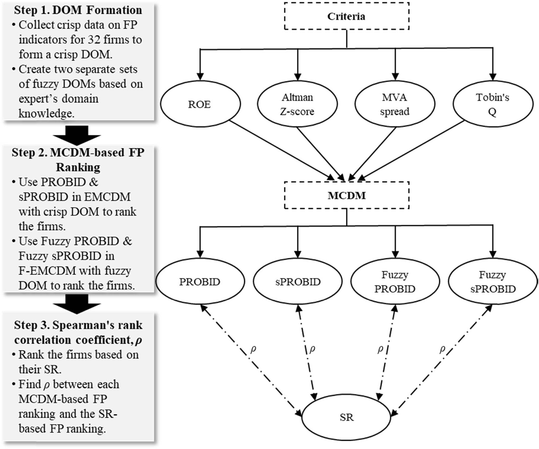
Flowchart illustrating the systematic approach to determine MCDM-based FP rankings using crisp and fuzzy DOMs, and find their Spearman’s rank correlation coefficient (ρ) with SR-based FP ranking.
4 Discussions and limitations
The calculated Spearman’s rank correlation coefficients between each MCDM-based FP ranking and the SR-based FP ranking are presented in a descending order in Figure 3. It is worth mentioning that the p-values of all Spearman’s rank correlation coefficients are less than 0.001, indicating high statistical significance and providing strong evidence to support the calculated correlation coefficients. These results reveal important insights regarding the performance of MCDM methods tested and different types of DOMs in this application. Specifically, first, when using the crisp DOM, sPROBID outperforms PROBID by leading to a higher correlation coefficient with the SR-based FP ranking (i.e., 0.655 vs 0.569). Second, fuzzy sPROBID performs better than fuzzy PROBID for both triangular and trapezoidal fuzzy DOMs. Third, the correlation results based on the fuzzy DOMs are consistently higher than those based on the crisp DOM. Fourth, fuzzy sPROBID provides slightly better correlation result with the triangular fuzzy DOM than with the trapezoidal fuzzy DOM (i.e., 0.770 vs 0.769), whereas fuzzy PROBID gives better correlation result with the trapezoidal fuzzy DOM than with the triangular fuzzy DOM (i.e., 0.704 vs 0.674). Finally and notably, fuzzy sPROBID with triangular fuzzy DOM performs the best overall, yielding a high Spearman’s rank correlation coefficient of 0.770 with the SR-based FP ranking.
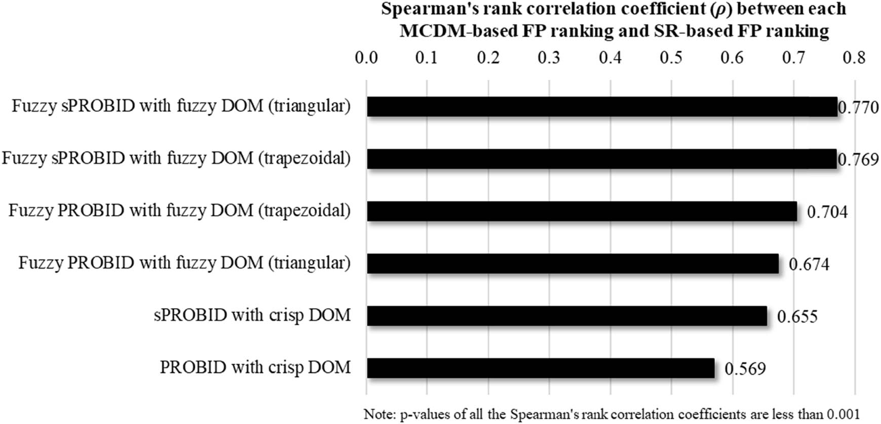
Descending order of Spearman’s rank correlation coefficient (ρ) between each MCDM-based FP ranking and SR-based FP ranking.
In addition, Sałabun and Urbaniak [36] recently proposed a new coefficient, termed the WS coefficient, to measure the similarity between two rankings. The key innovation of this coefficient is that positions at the top of the ranking have a more significant impact on the similarity than those at the bottom of the ranking. For instance, a reversal of alternatives between the first and second positions would be regarded as more impactful than a reversal between the fourth and fifth positions, during the similarity measurement process. On the other hand, Spearman’s rank correlation coefficient is indifferent to whether the reversals occur at the top or bottom of the ranking, treating each position with equal impact.
In this study, WS coefficient is also adopted to supplement the findings derived from the more commonly used Spearman’s rank correlation coefficient. Note that, in the present application, the WS coefficient values obtained are significantly higher than the Spearman’s rank correlation coefficient values, and the range of the former is less than that of the latter. This is because the top-ranked alternatives do not fluctuate significantly among the different rankings; these alternatives weigh more heavily when calculating the WS coefficient and lead to the overall higher WS coefficient values. Additionally, as seen from Figure 4, even when we account for the varied impacts of different positions using WS coefficient, the principal observation underscored by Spearman’s rank correlation coefficient from Figure 3 remains intact, i.e., the correlations (or similarities) based on the fuzzy DOMs are still consistently higher than those based on the crisp DOM. The remaining findings are largely congruent with those from Figure 3. For instance, when using crisp DOM, sPROBID outperforms PROBID by generating a slightly higher WS coefficient (i.e., 0.8552 vs 0.8543). Fuzzy sPROBID also performs slightly better than fuzzy PROBID for both triangular and trapezoidal fuzzy DOMs (i.e., 0.8823 vs 0.8821, and 0.8869 vs 0.8864).
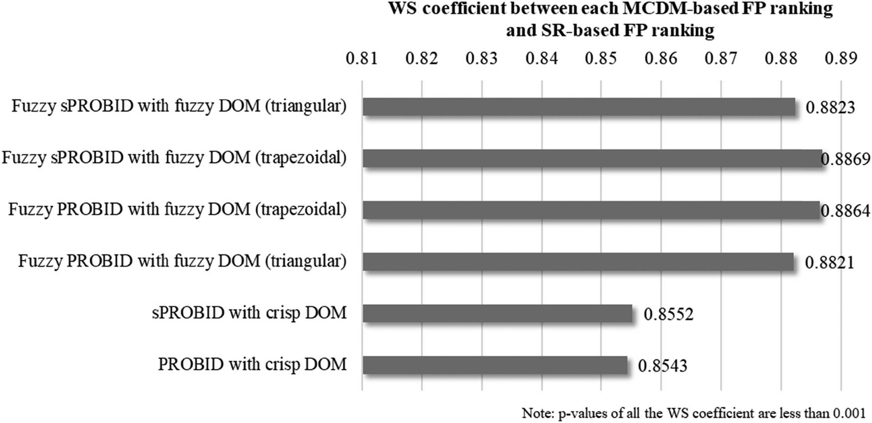
WS coefficient between each MCDM-based FP ranking and SR-based FP ranking.
The findings demonstrate the effectiveness of fuzzy DOM, not only under conditions of fuzzy information, but also in contexts where crisp numerical information is present. Indeed, financial experts interpret numerical information from balance sheets using their domain knowledge to form linguistic assessments. For instance, the financial expert consulted in this study prioritizes dynamic, time-varying ratios over static ones. Furthermore, financial experts are also acutely aware of the implications and significance of any increases or decreases in the FP criteria. The use of crisp DOM, however, does not always successfully navigate these complex and nonlinear cases. Implementing fuzzy techniques leads to a more flexible linguistic interpretation that incorporates the insights of decision makers/experts, thus facilitating the assessment of nonlinear situations. This flexibility is observed from the results obtained in the present study and is a key factor contributing to the superior performance of fuzzy MCDM methods coupled with fuzzy DOM in better representing real-world financial market situations.
Regarding limitations, this study is grounded in some static dimensions for financial data, including the use of MCDM methods, normalization technique, assigned weights, time range, criteria, and alternatives; any change in these may affect the final results to some extent. However, the focus of this study revolves around the proposed exploration of the selection between fuzzy and crisp DOM through comparisons with an identified objective benchmark, and the introduction of the new fuzzy PROBID and fuzzy sPROBID methods for fuzzy MCDM. The comparison between crisp and fuzzy DOM can be expanded to more MCDM methods, more objective benchmarks, and more problem scenarios.
5 Conclusions
In conclusion, accurate assessment of FP is crucial for informed decision-making in the financial market. MCDM methods are useful in evaluating trade-offs among multiple criteria and making informed decisions. Nonetheless, selecting the most appropriate MCDM method for a specific application remains a challenge. In this study, we took real-life SR-based ranking as the objective benchmark to compare FP rankings generated by different MCDM methods. We observed from the literature review that decision makers/experts, based on their domain knowledge, prefer to give fuzzy linguistic terms (instead of crisp numerical values) of criteria, to establish a fuzzy DOM. Fuzzy MCDM methods are then used to rank and select the best alternative. Moreover, previous publications have not adequately studied the selection between fuzzy and crisp DOM in MCDM. This work bridged the research gap through comparative analyses of fuzzy and crisp DOM in MCDM and also proposed two new fuzzy MCDM methods, namely, fuzzy PROBID and fuzzy sPROBID. These fuzzy methods coupled with fuzzy DOM produced higher correlation results with the SR-based FP ranking than their crisp counterparts. Fuzzy sPROBID with triangular fuzzy DOM produces a high Spearman’s rank correlation coefficient of 0.770 with the SR-based FP ranking. Our study advanced the investigation into the application of fuzzy MCDM methods and provided insights into the performance of MCDM methods tested with different types of DOMs (triangular fuzzy, trapezoidal fuzzy, and crisp). For future research, the proposed methodology in this work can be expanded to more MCDM methods, more objective benchmarks, and more problem scenarios.
-
Conflict of interest: Dr. Željko Stević is the Guest Editor of the “Special Issue on Development of Fuzzy Sets and Their Extensions”, but was not involved in the review process of this article.
References
[1] M. Baydaş, The effect of pandemic conditions on financial success rankings of BIST SME industrial companies: a different evaluation with the help of comparison of special capabilities of MOORA, MABAC and FUCA methods, Bus Manag Stud An Int J. 10 (2022), no. 1, 245–260.10.15295/bmij.v10i1.1997Search in Google Scholar
[2] O. Pala, A mixed-integer linear programming model for aggregating multi–criteria decision making methods, Decis Making Appl Manag Eng. 5 (2022), no. 2, 260–286.10.31181/dmame0318062022pSearch in Google Scholar
[3] M. Park, Z. Wang, L. Li, and X. Wang, Multi-objective building energy system optimization considering EV infrastructure, Appl Energy. 332 (2023), 120504.10.1016/j.apenergy.2022.120504Search in Google Scholar
[4] Ž Stević, D. K. Das, R. Tešić, M. Vidas, and D. Vojinović, Objective criticism and negative conclusions on using the fuzzy SWARA method in multi-criteria decision making, Mathematics 10 (2022), no. 4, 635.10.3390/math10040635Search in Google Scholar
[5] T. Turhan and E. Aydemir, A financial ratio analysis on BIST information and technology index (XUTEK) Using AHP-weighted grey relational analysis, Düzce Üniversitesi Bilim ve Teknoloji Derg. 9 (2021), no. 6, 195–209.10.29130/dubited.1011252Search in Google Scholar
[6] W. Zhang, X. Liu, W. Yu, C. Cui and A. Zheng, Spatial-temporal sensitivity analysis of flood control capability in china based on MADM-GIS model, Entropy 24 (2022), no. 6, 772.10.3390/e24060772Search in Google Scholar PubMed PubMed Central
[7] C. Zopounidis, E. Galariotis, M. Doumpos, S. Sarri and K. AndriosopouloS, Multiple criteria decision aiding for finance: An updated bibliographic survey, Eur J Operational Res. 247 (2015), no. 2, 339–348.10.1016/j.ejor.2015.05.032Search in Google Scholar
[8] Z. Wang, J. Li, G. P. Rangaiah and Z. Wu, Machine learning aided multi-objective optimization and multi-criteria decision making: Framework and two applications in chemical engineering, Comput Chem Eng. 165 (2022), 107945.10.1016/j.compchemeng.2022.107945Search in Google Scholar
[9] S. R. Nabavi, Z. Wang and G. P. Rangaiah, Sensitivity analysis of multi-criteria decision-making methods for engineering applications, Ind & Eng Chem Res. 62 (2023), no. 17, 6707–6722.10.1021/acs.iecr.2c04270Search in Google Scholar
[10] Z. Wang, S. R. Nabavi and G. P. Rangaiah, Selected multi-criteria decision-making methods and their applications to product and system design, Optimization Methods for Product and System Design, Springer, Singapore, 2023, 107–13810.1007/978-981-99-1521-7_7Search in Google Scholar
[11] S. Moslem, A novel parsimonious best worst method for evaluating travel mode choice, IEEE Access. 11 (2023), 16768–16773.10.1109/ACCESS.2023.3242120Search in Google Scholar
[12] Z. Wang, W. G. Y. Tan, G. P. Rangaiah and Z. Wu, Machine learning aided model predictive control with multi-objective optimization and multi-criteria decision making, Comput Chem Eng. 179 (2023), 108414, DOI: https://doi.org/10.1016/j.compchemeng.2023.108414.10.1016/j.compchemeng.2023.108414Search in Google Scholar
[13] S. R. Nabavi, M. J. Jafari and Z. Wang, Deep learning aided multi-objective optimization and multi-criteria decision making in thermal cracking process for olefines production, J Taiwan Inst Chem Eng. 152 (2023), 105179, DOI: 10.1016/j.jtice.2023.105179.10.1016/j.jtice.2023.105179Search in Google Scholar
[14] D. Danesh, M. J. Ryan and A. Abbasi, A systematic comparison of multi-criteria decision making methods for the improvement of project portfolio management in complex organisations, Int J Manag Decis Mak. 16 (2017), no. 3, 280–320.10.1504/IJMDM.2017.085638Search in Google Scholar
[15] M. Baydaş and D. Pamučar, Determining objective characteristics of MCDM methods under uncertainty: an exploration study with financial data, Mathematics 10 (2022), no. 7, 1115.10.3390/math10071115Search in Google Scholar
[16] A. Jusufbašić and Ž Stević, Measuring logistics service quality using the SERVQUAL model, J Intell Manag Decis. 2 (2023), 1–10.10.56578/jimd020101Search in Google Scholar
[17] Z. Wang and G. P. Rangaiah, Application and analysis of methods for selecting an optimal solution from the Pareto-optimal front obtained by multiobjective optimization, Ind & Eng Chem Res. 56 (2017), no. 2, 560–574.10.1021/acs.iecr.6b03453Search in Google Scholar
[18] S. Moslem, Ž Stević, I. Tanackov and F. Pilla, Sustainable development solutions of public transportation: An integrated IMF SWARA and Fuzzy Bonferroni operator, Sustain Cities Soc. 93 (2023), 104530.10.1016/j.scs.2023.104530Search in Google Scholar
[19] W. H. Lam, W. S. Lam, K. F. Liew and P. F. Lee, Decision analysis on the financial performance of companies using integrated entropy-fuzzy TOPSIS model, Mathematics 11 (2023), no. 2, 397.10.3390/math11020397Search in Google Scholar
[20] S. Raheja and V. Jain, Designing of a new intuitionistic fuzzy based diabetic diagnostic system, Int J Fuzzy Syst Appl (IJFSA). 7 (2018), no. 1, 32–45.10.4018/IJFSA.2018010103Search in Google Scholar
[21] A. S. Kumar and M. Kalpana, Emerging application of fuzzy expert system in medical domain, Fuzzy Expert Systems for Disease Diagnosis, IGI Global, Hershey, Pennsylvania, 2015, 1–20.10.4018/978-1-4666-7240-6.ch001Search in Google Scholar
[22] M. Baydaş and T. Eren, Finansal performans Ölçümünde ÇKKV Yöntem Seçimi Problemine Objektif Bir Yaklaşım: Borsa İstanbul’da Bir Uygulama, Eskişeh Osman Üniv İktis ve İdari Bilim Derg. 16 (2021), no. 3, 664–687.10.17153/oguiibf.947593Search in Google Scholar
[23] Z. Wang, G. P. Rangaiah and X. Wang, Preference ranking on the basis of ideal-average distance method for multi-criteria decision-making, Ind & Eng Chem Res 60 (2021), no. 30, 11216–11230.10.1021/acs.iecr.1c01413Search in Google Scholar
[24] A. P. Darko, C. O. Antwi, K. O. Asamoah, E. Opoku-Mensah and J. Ren, A probabilistic reliable linguistic PROBID method for selecting electronic mental health platforms considering users’ bounded rationality, Eng Appl Artif Intell. 125 (2023), 106716.10.1016/j.engappai.2023.106716Search in Google Scholar
[25] M. Dai, H. Yang, J. Wang, F. Yang, Z. Zhang, Y. Yu, et al., Energetic, economic and environmental (3E) optimization of hydrogen production process from coal-biomass co-gasification based on a novel method of Ordering Preference Targeting at Bi-Ideal Average Solutions (OPTBIAS), Comput Chem Eng. 169 (2023), 108084.10.1016/j.compchemeng.2022.108084Search in Google Scholar
[26] M. Yurdakul and Y. T. İç, Comparison of fuzzy and crisp versions of an AHP and TOPSIS model for nontraditional manufacturing process ranking decision, J Adv Manuf Syst. 18 (2019), no. 2, 167–192.10.1142/S0219686719500094Search in Google Scholar
[27] B. Kizielewicz and A. Bączkiewicz, Comparison of Fuzzy TOPSIS, Fuzzy VIKOR, Fuzzy WASPAS and Fuzzy MMOORA methods in the housing selection problem, Procedia Comput Sci. 192 (2021), 4578–4591.10.1016/j.procs.2021.09.236Search in Google Scholar
[28] G. Petrović, J. Mihajlović, Ž Ćojbašić, M. Madić and D. Marinković, Comparison of three fuzzy MCDM methods for solving the supplier selection problem, Facta Universitatis, Series: Mech Eng. 17 (2019), no. 3, 455–469.10.22190/FUME190420039PSearch in Google Scholar
[29] R. Zamani, A. M. A. Ali and A. Roozbahani, Evaluation of adaptation scenarios for climate change impacts on agricultural water allocation using fuzzy MCDM methods, Water Resour Manag. 34 (2020), 1093–1110,10.1007/s11269-020-02486-8Search in Google Scholar
[30] S. Kumar, S. R. Maity and L. Patnaik, Optimization of wear parameters for Duplex-TiAlN coated MDC-K tool steel using fuzzy mcdm techniques, Oper Res Eng Sci Theory Appl. 5 (2022), no. 3, 40–67.10.31181/110722105kSearch in Google Scholar
[31] S. Ahmad, S. Masood, N. Z. Khan, I. A. Badruddin, A. Ahmadian, Z. A. Khan, et al., Analysing the impact of COVID-19 pandemic on the psychological health of people using fuzzy MCDM methods, Oper Res Perspect. 10 (2023), 100263.10.1016/j.orp.2022.100263Search in Google Scholar
[32] E. A. Adalı, T. Öztaş, A. Özçil, G. Z. Öztaş and A. Tuş, A new multi-criteria decision-making method under neutrosophic environment: ARAS method with single-valued neutrosophic numbers, Int J Inf Technol & Decis Mak. 22 (2023), no. 1, 57–87.10.1142/S0219622022500456Search in Google Scholar
[33] M. Baydaş, T. Eren, Ž Stević, V. Starčević and R. Parlakkaya, Proposal for an objective binary benchmarking framework that validates each other for comparing MCDM methods through data analytics, PeerJ Comput Sci. 9 (2023), e1350.10.7717/peerj-cs.1350Search in Google Scholar PubMed PubMed Central
[34] Z. Wang, S. S. Parhi, G. P. Rangaiah and A. K. Jana, Analysis of weighting and selection methods for pareto-optimal solutions of multiobjective optimization in chemical engineering applications, Ind & Eng Chem Res. 59 (2020), no. 33, 14850–14867.10.1021/acs.iecr.0c00969Search in Google Scholar
[35] Z. Wang, S. A. Irfan, C. Teoh and P. H. Bhoyar, Numerical Machine Learning, Bentham Science Publishers, Singapore, 2023. DOI: https://doi.org/10.2174/9789815136982123010001.10.2174/97898151369821230101Search in Google Scholar
[36] W. Sałabun and K. Urbaniak, A new coefficient of rankings similarity in decision-making problems, Computational Science–ICCS 202020th International Conference, Amsterdam, The Netherlands, June 3–5, 2020, Proceedings, Part II 20, 2020, Springer, pp. 632–64510.1007/978-3-030-50417-5_47Search in Google Scholar
© 2023 the author(s), published by De Gruyter
This work is licensed under the Creative Commons Attribution 4.0 International License.
Articles in the same Issue
- Regular Articles
- A novel class of bipolar soft separation axioms concerning crisp points
- Duality for convolution on subclasses of analytic functions and weighted integral operators
- Existence of a solution to an infinite system of weighted fractional integral equations of a function with respect to another function via a measure of noncompactness
- On the existence of nonnegative radial solutions for Dirichlet exterior problems on the Heisenberg group
- Hyers-Ulam stability of isometries on bounded domains-II
- Asymptotic study of Leray solution of 3D-Navier-Stokes equations with exponential damping
- Semi-Hyers-Ulam-Rassias stability for an integro-differential equation of order 𝓃
- Jordan triple (α,β)-higher ∗-derivations on semiprime rings
- The asymptotic behaviors of solutions for higher-order (m1, m2)-coupled Kirchhoff models with nonlinear strong damping
- Approximation of the image of the Lp ball under Hilbert-Schmidt integral operator
- Best proximity points in ℱ-metric spaces with applications
- Approximation spaces inspired by subset rough neighborhoods with applications
- A numerical Haar wavelet-finite difference hybrid method and its convergence for nonlinear hyperbolic partial differential equation
- A novel conservative numerical approximation scheme for the Rosenau-Kawahara equation
- Fekete-Szegö functional for a class of non-Bazilevic functions related to quasi-subordination
-
On local fractional integral inequalities via generalized
- On some geometric results for generalized k-Bessel functions
- Convergence analysis of M-iteration for 𝒢-nonexpansive mappings with directed graphs applicable in image deblurring and signal recovering problems
- Some results of homogeneous expansions for a class of biholomorphic mappings defined on a Reinhardt domain in ℂn
- Graded weakly 1-absorbing primary ideals
- The existence and uniqueness of solutions to a functional equation arising in psychological learning theory
- Some aspects of the n-ary orthogonal and b(αn,βn)-best approximations of b(αn,βn)-hypermetric spaces over Banach algebras
- Numerical solution of a malignant invasion model using some finite difference methods
- Increasing property and logarithmic convexity of functions involving Dirichlet lambda function
- Feature fusion-based text information mining method for natural scenes
- Global optimum solutions for a system of (k, ψ)-Hilfer fractional differential equations: Best proximity point approach
- The study of solutions for several systems of PDDEs with two complex variables
- Regularity criteria via horizontal component of velocity for the Boussinesq equations in anisotropic Lorentz spaces
- Generalized Stević-Sharma operators from the minimal Möbius invariant space into Bloch-type spaces
- On initial value problem for elliptic equation on the plane under Caputo derivative
- A dimension expanded preconditioning technique for block two-by-two linear equations
- Asymptotic behavior of Fréchet functional equation and some characterizations of inner product spaces
- Small perturbations of critical nonlocal equations with variable exponents
- Dynamical property of hyperspace on uniform space
- Some notes on graded weakly 1-absorbing primary ideals
- On the problem of detecting source points acting on a fluid
- Integral transforms involving a generalized k-Bessel function
- Ruled real hypersurfaces in the complex hyperbolic quadric
- On the monotonic properties and oscillatory behavior of solutions of neutral differential equations
- Approximate multi-variable bi-Jensen-type mappings
- Mixed-type SP-iteration for asymptotically nonexpansive mappings in hyperbolic spaces
- On the equation fn + (f″)m ≡ 1
- Results on the modified degenerate Laplace-type integral associated with applications involving fractional kinetic equations
- Characterizations of entire solutions for the system of Fermat-type binomial and trinomial shift equations in ℂn#
- Commentary
- On I. Meghea and C. S. Stamin review article “Remarks on some variants of minimal point theorem and Ekeland variational principle with applications,” Demonstratio Mathematica 2022; 55: 354–379
- Special Issue on Fixed Point Theory and Applications to Various Differential/Integral Equations - Part II
- On Cauchy problem for pseudo-parabolic equation with Caputo-Fabrizio operator
- Fixed-point results for convex orbital operators
- Asymptotic stability of equilibria for difference equations via fixed points of enriched Prešić operators
- Asymptotic behavior of resolvents of equilibrium problems on complete geodesic spaces
- A system of additive functional equations in complex Banach algebras
- New inertial forward–backward algorithm for convex minimization with applications
- Uniqueness of solutions for a ψ-Hilfer fractional integral boundary value problem with the p-Laplacian operator
- Analysis of Cauchy problem with fractal-fractional differential operators
- Common best proximity points for a pair of mappings with certain dominating property
- Investigation of hybrid fractional q-integro-difference equations supplemented with nonlocal q-integral boundary conditions
- The structure of fuzzy fractals generated by an orbital fuzzy iterated function system
- On the structure of self-affine Jordan arcs in ℝ2
- Solvability for a system of Hadamard-type hybrid fractional differential inclusions
- Three solutions for discrete anisotropic Kirchhoff-type problems
- On split generalized equilibrium problem with multiple output sets and common fixed points problem
- Special Issue on Computational and Numerical Methods for Special Functions - Part II
- Sandwich-type results regarding Riemann-Liouville fractional integral of q-hypergeometric function
- Certain aspects of Nörlund ℐ-statistical convergence of sequences in neutrosophic normed spaces
- On completeness of weak eigenfunctions for multi-interval Sturm-Liouville equations with boundary-interface conditions
- Some identities on generalized harmonic numbers and generalized harmonic functions
- Study of degenerate derangement polynomials by λ-umbral calculus
- Normal ordering associated with λ-Stirling numbers in λ-shift algebra
- Analytical and numerical analysis of damped harmonic oscillator model with nonlocal operators
- Compositions of positive integers with 2s and 3s
- Kinematic-geometry of a line trajectory and the invariants of the axodes
- Hahn Laplace transform and its applications
- Discrete complementary exponential and sine integral functions
- Special Issue on Recent Methods in Approximation Theory - Part II
- On the order of approximation by modified summation-integral-type operators based on two parameters
- Bernstein-type operators on elliptic domain and their interpolation properties
- A class of strongly convergent subgradient extragradient methods for solving quasimonotone variational inequalities
- Special Issue on Recent Advances in Fractional Calculus and Nonlinear Fractional Evaluation Equations - Part II
- Application of fractional quantum calculus on coupled hybrid differential systems within the sequential Caputo fractional q-derivatives
- On some conformable boundary value problems in the setting of a new generalized conformable fractional derivative
- A certain class of fractional difference equations with damping: Oscillatory properties
- Weighted Hermite-Hadamard inequalities for r-times differentiable preinvex functions for k-fractional integrals
- Special Issue on Recent Advances for Computational and Mathematical Methods in Scientific Problems - Part II
- The behavior of hidden bifurcation in 2D scroll via saturated function series controlled by a coefficient harmonic linearization method
- Phase portraits of two classes of quadratic differential systems exhibiting as solutions two cubic algebraic curves
- Petri net analysis of a queueing inventory system with orbital search by the server
- Asymptotic stability of an epidemiological fractional reaction-diffusion model
- On the stability of a strongly stabilizing control for degenerate systems in Hilbert spaces
- Special Issue on Application of Fractional Calculus: Mathematical Modeling and Control - Part I
- New conticrete inequalities of the Hermite-Hadamard-Jensen-Mercer type in terms of generalized conformable fractional operators via majorization
- Pell-Lucas polynomials for numerical treatment of the nonlinear fractional-order Duffing equation
- Impacts of Brownian motion and fractional derivative on the solutions of the stochastic fractional Davey-Stewartson equations
- Some results on fractional Hahn difference boundary value problems
- Properties of a subclass of analytic functions defined by Riemann-Liouville fractional integral applied to convolution product of multiplier transformation and Ruscheweyh derivative
- Special Issue on Development of Fuzzy Sets and Their Extensions - Part I
- The cross-border e-commerce platform selection based on the probabilistic dual hesitant fuzzy generalized dice similarity measures
- Comparison of fuzzy and crisp decision matrices: An evaluation on PROBID and sPROBID multi-criteria decision-making methods
- Rejection and symmetric difference of bipolar picture fuzzy graph