Phase portraits of two classes of quadratic differential systems exhibiting as solutions two cubic algebraic curves

Rebiha Benterki; Ahlam Belfar

doi:10.1515/dema-2022-0218

Artikel Open Access

Phase portraits of two classes of quadratic differential systems exhibiting as solutions two cubic algebraic curves

Rebiha Benterki und Ahlam Belfar

Veröffentlicht/Copyright: 25. Mai 2023

Veröffentlicht von

Veröffentlichen auch Sie bei De Gruyter Brill

Informationen für Autor*innen Erkunden Sie dieses Fachgebiet

Aus der Zeitschrift Demonstratio Mathematica Band 56 Heft 1

Abstract

The classification of the phase portraits is one of the classical and difficult problems in the qualitative theory of polynomial differential systems in R 2 , particularly for quadratic systems. Even with the hundreds of studies on the topology of real planar quadratic vector fields, fully characterizing their phase portraits is still a difficult problem. This paper is devoted to classifying the phase portraits of two polynomial vector fields with two usual invariant algebraic curves, by investigating the geometric solutions within the Poincaré disc. One can notice that these systems yield 26 topologically different phase portraits.

Keywords: polynomial vector fields; phase portrait; invariant curve

MSC 2010: 34C07; 34C29; 34A26

1 Introduction and statement of the main results

A differential system on the plane is called a polynomial vector field if the following equations hold:

(1) x ˙ = P ( x , y ) , y ˙ = Q ( x , y ) ,

where P and Q are two polynomials depending on variables x and y over R , and the degree of system (1) is the integer n = max { deg ( P ) , deg ( Q ) } . If n = 2 , the system is called a quadratic differential system, which will be denoted in our article by QS. This type of differential system is used in modeling many natural phenomena described in several disciplines of science, as well as in biological and physical applications. In addition to their use, quadratic differential systems also attracted the attention of mathematicians. It is well known that there is a relation between the theory of polynomial differential systems and algebraic curves. The existence of a certain number of algebraic curves enables the determination of the differential system’s first integral.

We define an algebraic invariant curve h ( x , y ) = 0 of system (1), with h ( x , y ) ∈ R [ x , y ] , as an algebraic curve satisfying the following partial differential equation:

P ( x , y ) ∂ h ∂ x + Q ( x , y ) ∂ h ∂ y = k ( x , y ) h ( x , y ) ,

where k ( x , y ) is a polynomial depending on two variables x and y with degree 0 or 1, which is the cofactor of h ( x , y ) = 0 , for more details see [1].

The papers studying the QS have been extensively investigated, and the literature about them is abundant, see [2,3,4, 5,6]. The first articles came to light in 1960 interested in the classification of global dynamics of QS, the fact that these systems depend on 12 parameters made them difficult to study. For this reason, the authors studied and classified the global phase portraits of some particular classes of QS. The first class studied is the classification of quadratic centers and their first integrals, which began with the works of Dulac [7], Kapteyn [8,9], Bautin [10], Lunkevich and Sibirskii [11], Ye and Ye [12], Artès et al. [13]. For the class of the homogeneous quadratic systems, see for example the works of Lyagina [14], Sibirskii and Vulpe [15], and Newton [16].

Recently, Benterki and Llibre [17] classified the global dynamics of 14 QS exhibiting some relevant classical algebraic curves of degree 4 and provided 31 topologically different phase portraits in the Poincaré disc for these systems. In another study, Belfar and Benterki [18] classified the global dynamics of five QS with at most two parameters, exhibiting five well-known algebraic curves of degree three and proved that these systems exhibit 29 topologically different phase portraits.

This article is a continuation of the study done by Belfar and Benterki [18], where we classified the phase portraits in the Poincaré disk of two QS with at most four parameters, exhibiting two classical invariant algebraic curves of degree 3, and it is easily perceived that these differential systems possess 26 topologically non-equivalent phase portraits. More precisely, we analyze the quadratic differential systems having usual cubic invariant curves.

In the following theorem we present a normal form for any differential quadratic polynomial systems possessing Cubical Hyperbola or Semicubical Parabola invariant curves.

Theorem 1

The cubic algebraic curve Cubical Hyperbola h 1 ( x , y ) = x y 2 − ( x + 1 ) 2 , having a cofactor k 1 ( x , y ) = 2 a x , is invariant of the QS
(2) x ˙ = a x + a x 2 − 2 x y , y ˙ = − 2 − 2 x − a y 2 + a x y 2 + y 2 .
The cubic algebraic curve Semicubical Parabola h 2 ( x , y ) = y 2 − a x 3 , where a ≠ 0 , with cofactor k 2 ( x , y ) = c + x + b y , is invariant of the QS
(3) x ˙ = c x 3 + d y + x 2 3 + b x y 3 , y ˙ = c y 2 + 3 a d x 2 2 + x y 2 + b y 2 2 .
For more details about invariant cubic curves realizable by quadratic differential systems see [19].

Remark 2

Rather than studying the systems mentioned in Theorem 1 for all their parameter values, we restrict ourselves by carrying out the next symmetries.

Systems (2) are invariant over the change ( x , y , t , a ) → ( x , − y , − t , − a ) , then we can study these systems only for a ⩾ 0 .
Systems (3) are invariant over the change ( x , y , t , a , b , c , d ) → ( x , − y , t , a , − b , c , − d ) , then we can study these systems only for b > 0 or ( b = 0 and d ⩾ 0 ).

The following theorem presents the geometric solutions of the two systems mentioned in Theorem 1.

Theorem 3

The global dynamics in the Poincaré disc of the two vector fields given in Theorem 1 are given in Figures 1–3. More precisely, we have the phase portrait

for systems (2) when a = 0 .
for systems (2) when a ∈ ( 0 , ∞ ) .
for systems (3) when d = 0 , b = 0 , and c ∈ R .
for systems (3) when d = 0 , b ≠ 0 , and c ∈ R .
for systems (3) when d ≠ 0 , b = 0 , and c = 0 .
for systems (3) when 1 − 36 a b d > 0 , a d < 0 , b c ≠ 0 , and δ 1 = ( − 27 a 2 b 2 c 2 − 9 a 2 d 2 ( 12 a b d − 1 ) − a c ( 4 − 54 a b d ) ) > 0 .
for systems (3) when 1 − 36 a b d > 0 , a d < 0 , b c ≠ 0 , and δ 1 = 0 .
for systems (3) when 1 − 36 a b d > 0 , a d < 0 , b c ≠ 0 , and δ 1 < 0 .
for systems (3) when 1 − 36 a b d > 0 , a d > 0 , b c ≠ 0 , and δ 1 > 0 .
for systems (3) when 1 − 36 a b d > 0 , a d > 0 , b c ≠ 0 , and δ 1 = 0 .
for systems (3) when 1 − 36 a b d > 0 , a d > 0 , b c ≠ 0 , and δ 1 < 0 .
for systems (3) when 1 − 36 a b d = 0 , b c ≠ 0 , and δ 2 = ( 1 / 216 ) b 2 − ( 5 a c ) / 2 − 27 a 2 b 2 c 2 > 0 .
for systems (3) when 1 − 36 a b d = 0 , b c ≠ 0 , and δ 2 = 0 .
for systems (3) when 1 − 36 a b d = 0 , b c ≠ 0 , and δ 2 < 0 .
for systems (3) when 1 − 36 a b d < 0 , b c ≠ 0 , and δ 1 > 0 .
for systems (3) when 1 − 36 a b d < 0 , b c ≠ 0 , and δ 1 = 0 , or 1 − 36 a b d < 0 , b ≠ 0 , c = 0 , and δ 3 > 0 .
for systems (3) when 1 − 36 a b d < 0 , b c ≠ 0 , and δ 1 < 0 .
for systems (3) when 1 − 36 a b d > 0 , a d > 0 , b ≠ 0 , c = 0 , and δ 3 = 1 − 12 a b d > 0 .
for systems (3) when 1 − 36 a b d > 0 , a d < 0 , b ≠ 0 , c = 0 , and δ 3 > 0 .
for systems (3) when 1 − 36 a b d < 0 , b ≠ 0 , c = 0 , and δ 3 > 0 .
for systems (3) when 1 − 36 a b d < 0 , b ≠ 0 , c = 0 , and δ 3 = 0 .
for systems (3) when 1 − 36 a b d < 0 , b ≠ 0 , c = 0 , and δ 3 < 0 .
for systems (3) when 1 − 36 a b d = 0 , b ≠ 0 , c = 0 , and δ 4 = 121 216 ( a 2 b 2 ) > 0 .
for systems (3) when b = 0 , d c ≠ 0 , and δ 5 = 9 a d 2 − 4 c > 0 .
for systems (3) when b = 0 , d c ≠ 0 , and δ 5 = 0 .
for systems (3) when b = 0 , d c ≠ 0 , and δ 5 < 0 .

Figure 1

Geometric solutions of systems (2) and (3).

Figure 2

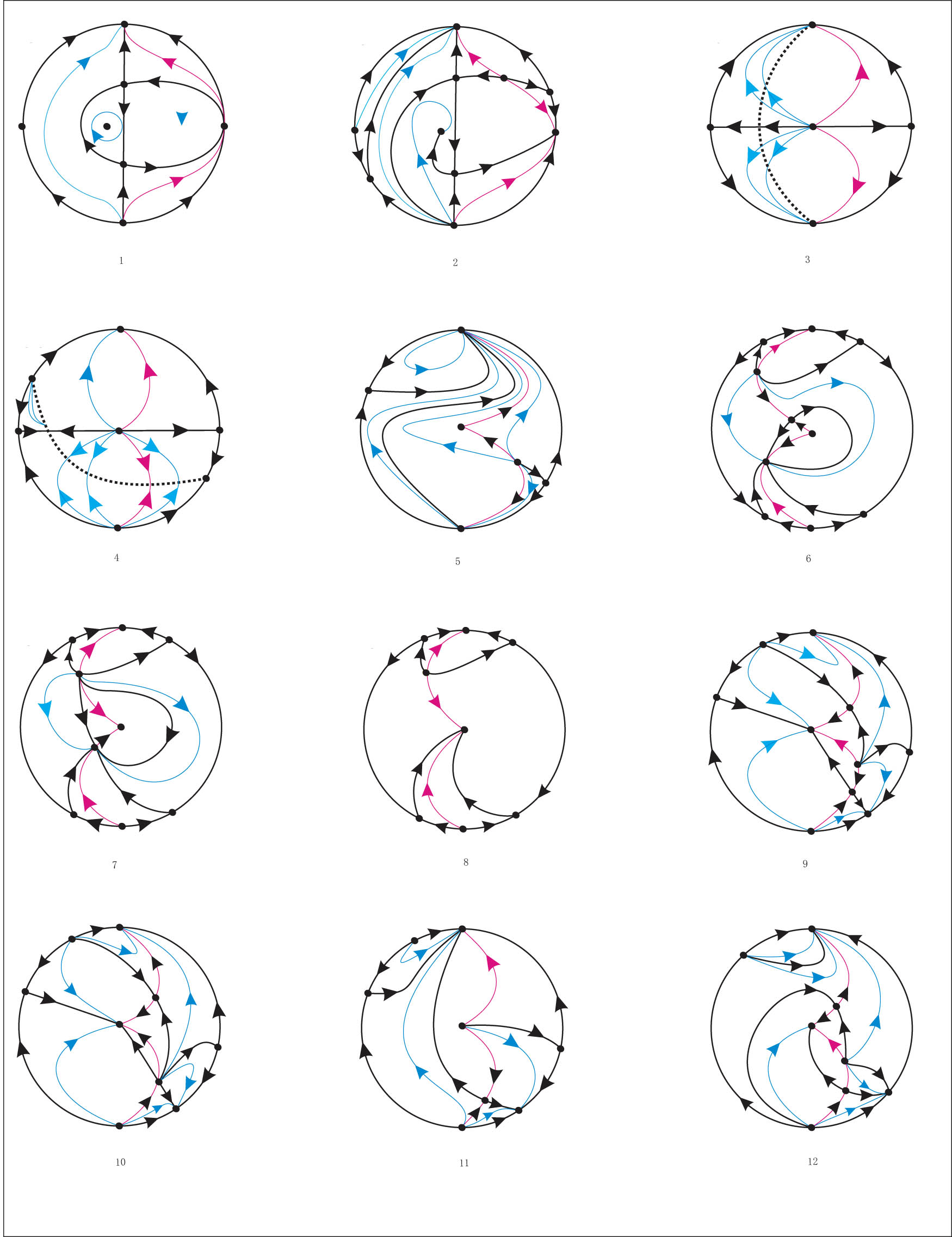
Continuation of Figure 1.

Figure 3

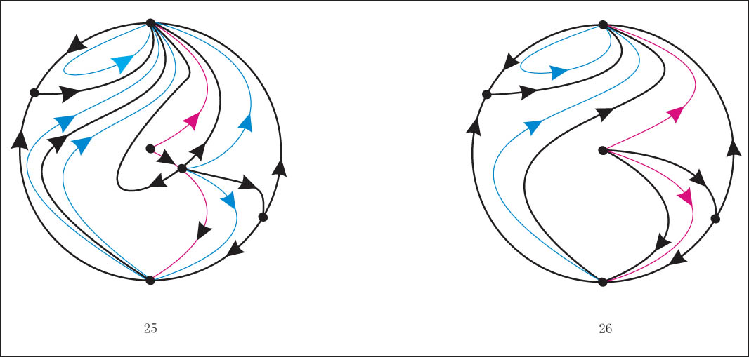
Continuation of Figure 1.

2 Preliminaries and fundamental results

In this section, we present some fundamental tools we need to analyze the behavior of the trajectories of planar vector fields.

2.1 Geometric solutions within the Poincaré disc

In this part, we present some fundamental findings that are essential for understanding how a planar polynomial differential system’s trajectories behave when it approaches infinity. Let X ( x , y ) = ( P ( x , y ) , Q ( x , y ) ) be a polynomial vector field of degree n . We consider the Poincaré sphere S 2 = { ( y 1 , y 2 , y 3 ) ∈ R 3 : y 1 2 + y 2 2 + y 3 2 = 1 } . We identify the plane R 2 , where we have defined the polynomial vector field X , with the tangent plane T ( 0 , 0 , 1 ) S 2 to the sphere S 2 at the north pole ( 0 , 0 , 1 ) . We consider the central projection f : T ( 0 , 0 , 1 ) S 2 ⟶ S 2 such that, to each point of the plane q ∈ T ( 0 , 0 , 1 ) S 2 , f associates the two intersection points of the straight line that connects the points q and ( 0 , 0 , 0 ) with the sphere S 2 .

The equator S 1 = { ( y 1 , y 2 , y 3 ) ∈ S 2 : y 3 = 0 } corresponds to the infinity points of the plane R 2 ≡ T ( 0 , 0 , 1 ) S 2 . In conclusion, a vector field is obtained as follows X ′ which is defined in S 2 ⧹ S 1 , and created from two symmetric copies of X , one in the northern hemisphere and the other in the southern hemisphere. By scaling the vector field X by y 3 n , we can extend it to a vector field p ( X ) on S . We may determine the dynamics of p ( X ) close to infinity by looking at the dynamics of p ( X ) near S .

Since we need to do calculations on the Poincaré sphere, we consider the local charts U i = { ( y 1 , y 2 , y 3 ) ∈ S 2 : y i > 0 } and V i = { ( y 1 , y 2 , y 3 ) ∈ S 2 : y i < 0 } for i = 1 , 2 , 3 , with the associated diffeomorphisms F k : U i ⟶ R 2 and G k : V i ⟶ R 2 for k = 1 , 2 , 3 , where F k ( y 1 , y 2 , y 3 ) = − G k ( y 1 , y 2 , y 3 ) = ( y m / y k , y n / y k ) for m < n and m , n ≠ k . Let z = ( u , v ) be the value of F k ( y 1 , y 2 , y 3 ) or G k ( y 1 , y 2 , y 3 ) for any k ; note that the coordinates ( u , v ) play different roles depending on the local chart with which we are working. In the local charts U 1 , U 2 , V 1 , and V 2 , the points ( u , v ) corresponding to the infinity have its coordinate v = 0 .

After a scaling of the independent variable in the local chart ( U 1 , F 1 ) , the expression for p ( X ) is

u ˙ = v n − u P 1 v , u v + Q 1 v , u v , v ˙ = − v n + 1 P 1 v , u v ;

in the local chart ( U 2 , F 2 ) , the expression for p ( X ) is

u ˙ = v n P u v , 1 v − u Q u v , 1 v , v ˙ = − v n + 1 Q u v , 1 v ;

and for the local chart ( U 3 , F 3 ) the expression for p ( X ) is

u ˙ = P ( u , v ) , v ˙ = Q ( u , v ) .

Note that for studying the singular points at infinity, we only need to study the infinite singular points of the chart U 1 and the origin of the chart U 2 because the singular points at infinity appear in pairs diametrically opposite.

For more details on the Poincaré compactification, see Chapter 5 of [1].

An orbit that is a singular point, limit cycle, or a trajectory that lies in the boundary of a hyperbolic sector at a singular point is a separatrix of p ( X ) . The set formed by all separatrices of p ( X ) , designated by S ( p ( X ) ) , is closed, according to Neumann’s proof in [20].

Canonical regions of p ( X ) refer to the open connected components of D 2 ⧹ S ( p ( X ) ) . One solution selected from each canonical region is added to the union of S ( p ( X ) ) to form the separatrix configuration. It is argued that two separatrix configurations S ( p ( X ) ) and S ( p ( Y ) ) are topologically identical if an orientation-preserving or -reversing homeomorphism converts the trajectories of S ( p ( X ) ) into the trajectories of S ( p ( Y ) ) .

The following result was achieved by Neumann [20], Markus [21], and Peixoto [22].

Theorem 4

The phase portraits in the Poincaré disc of the two compactified polynomial differential systems p ( X ) and p ( Y ) are topologically equivalent if and only if their separatrix configurations S ( p ( X ) ) and S ( p ( Y ) ) are topologically equivalent.

Finally, for a precise definition of the index of singular points, see Chapter 6 of [1], but, for our intents, the next theorems known as the Poincaré formula give sufficient information about the subject. Then, to know the nature of a singular point, we can calculate its index, which is given in the following theorem.

Theorem 5

[Poincaré index formula] Let q be an isolated singular point having the finite sectorial decomposition property. Let e, h, and p denote the number of elliptic, hyperbolic, and parabolic sectors of q, respectively, and suppose that e + h + p > 0 Then, i q = ( e − h ) / 2 + 1 .

Theorem 6

[Poincaré-Hopf theorem] For every tangent vector field on S 2 with a finite number of singular points, the sum of their indices is 2.

3 Finite and infinite singularities

The singular points (or simply SP) of the two quadratic systems mentioned in Theorem 1 are given in the following proposition.

Proposition 7

The next assertions are valid for systems (2) and (3).

If a ∈ ( 0 , ∞ ) , systems (2) have four hyperbolic singularities: a stable focus at q 1 = ( − 1 , 0 ) , an unstable node at q 2 = ( 4 / a 2 , 2 / a + a / 2 ) , and two saddles at q 3 , 4 = ( 0 , ( a ± a 2 + 32 ) / 4 ) . If a = 0 , systems (2) have three finite SP: a centre at q 1 and two hyperbolic saddles at q 3 , 4 = ( 0 , ± 2 ) .
In U 1 and if a ≠ 0 , systems (2) have two hyperbolic singularities: a stable node at p 1 = ( 0 , 0 ) and a saddle at p 2 = ( a / 6 , 0 ) . If a = 0 , it has one nilpotent SP at the origin, where its local geometric solution is formed by two parabolic, two elliptic, and two hyperbolic sectors. The origin of U 2 is an hyperbolic stable node for a ⩾ 0 .
Assume a d < 0 and c ≠ 0 . In this case we have 1 − 36 a b d > 0 and systems (3) in the local chart U 1 have two hyperbolic saddles at p 1 , 2 = ( ( ± 1 − 36 a b d − 1 ) / ( 2 b ) , 0 ) . The origin of the local chart U 2 is an hyperbolic stable node for all a d ≠ 0 .
If δ 1 = − 27 a 2 b 2 c 2 − 9 a 2 d 2 ( 12 a b d − 1 ) − a c ( 4 − 54 a b d ) > 0 , systems (3) have four hyperbolic finite SP: the origin which is a node, a saddle, and two nodes.
If δ 1 = 0 , the systems have in addition to the origin, which is a node, two other SP: a node and a saddle-node.
If δ 1 < 0 , the systems have further to the node at q 1 = ( 0 , 0 ) , a second node that is stable when c ∈ ( − ∞ , 0 ) .
Assume 1 − 36 a b d > 0 , c ≠ 0 , and a d > 0 , systems (3) in the local chart U 1 have two hyperbolic SP: a saddle at p 1 = ( ( 1 − 36 a b d − 1 ) / ( 2 b ) , 0 ) and a stable node at p 2 = ( ( − 1 − 36 a b d − 1 ) / ( 2 b ) , 0 ) .
If δ 1 > 0 , the systems have further to the hyperbolic node at q 1 = ( 0 , 0 ) three hyperbolic singularities: a node and two saddles.
If δ 1 = 0 , the systems have in addition to the hyperbolic node at q 1 = ( 0 , 0 ) two singularities: a saddle-node and an hyperbolic saddle.
If δ 1 < 0 , the systems have two hyperbolic finite SP: a node at q 1 = ( 0 , 0 ) and a saddle.
Assume 1 − 36 a b d < 0 and c ≠ 0 , the systems have no singularity in the chart U 1 and the origin of U 2 is a stable-node.
If δ 1 > 0 , systems (3) have four hyperbolic finite SP: two nodes and two saddles.
If δ 1 = 0 , the systems have three finite SP: a node at q 1 = ( 0 , 0 ) , a saddle, and a semi-hyperbolic saddle node.
If δ 1 < 0 , systems (3) have two hyperbolic finite SP: a node at q 1 = ( 0 , 0 ) and a saddle.
Assume 1 − 36 a b d = 0 and c ≠ 0 , systems (3) have a semi-hyperbolic saddle-node at p 1 = p 2 = ( − 1 / ( 2 b ) , 0 ) and the origin of U 2 is a stable node.
If δ 2 = ( 1 / ( 216 b 2 ) − 27 a 2 b 2 c 2 − ( 5 a c ) / 2 ) > 0 , the systems have four hyperbolic finite SP: two nodes one at q 1 = ( 0 , 0 ) and two saddles.
If δ 2 = 0 , the systems have in addition to the hyperbolic node at q 1 = ( 0 , 0 ) two singularities: a saddle-node, and an hyperbolic saddle.
If δ 2 < 0 , the systems have two hyperbolic finite SP: a node at q 1 = ( 0 , 0 ) and a saddle.
Assume 1 − 36 a b d > 0 , c = 0 , and a d < 0 , systems (3) in the local chart U 1 have two hyperbolic saddles at p 1 , 2 = ( ( ± 1 − 36 a b d − 1 ) / ( 2 b ) , 0 ) and the origin of U 2 is an hyperbolic stable node for a d ≠ 0 . Since δ 3 = 1 − 12 a b d > 0 , the systems have three finite SP: the origin that is a cusp and two hyperbolic nodes.
Assume 1 − 36 a b d > 0 , c = 0 , and a d > 0 , systems (3) in the local chart U 1 have two hyperbolic SP: a saddle at p 1 = ( ( 1 − 36 a b d − 1 ) / ( 2 b ) , 0 ) and a stable node at p 2 = ( ( − 1 − 36 a b d − 1 ) / ( 2 b ) , 0 ) . Since δ 3 > 0 , the systems have in addition to the origin two hyperbolic finite singularities: a node and a saddle.
If 1 − 36 a b d = 0 and c = 0 , the systems in the chart U 1 have a semi-hyperbolic saddle-node at p 1 = p 2 = ( − 1 / ( 2 b ) , 0 ) and the origin of U 2 is a stable node. Since δ 4 = ( 121 a 2 b 6 ) / 216 > 0 , the systems have in addition to the origin two finite singularities: q 2 = ( ( 5 − 2 6 ) / ( 12 a b 2 ) , ( 11 6 − 27 ) / ( 72 a b 3 ) ) , which is an unstable node when a ∈ ( 0 , ∞ ) and a stable node when a ∈ ( − ∞ , 0 ) , and a saddle at q 3 = ( 5 + 2 6 ) / ( 12 a b 2 ) , ( − 27 − 11 6 ) / ( 72 a b 3 ) .
Assume 1 − 36 a b d < 0 and c = 0 , systems (3) have no singularity in the chart U 1 and the origin of the chart U 2 is a stable node.
If δ 3 > 0 , systems (3) have three finite SP: q 1 = ( 0 , 0 ) as in the previous case, one hyperbolic node, and one hyperbolic saddle.
If δ 3 = 0 , in addition to the origin, the systems have a semi-hyperbolic saddle-node at the point q 4 = ( 1 / ( 4 a b 2 ) , − 1 / ( 8 a b 3 ) ) .
If δ 3 < 0 , the systems have one finite cusp at the origin.
If d = 0 , b ≠ 0 , and c ∈ R , systems (3) have x + b y + c = 0 as a line of singularities, and by doing the change of variables ( x + b y + c ) d t = d s , we know that systems (3) have an unstable node at q 1 = ( 0 , 0 ) .
In U 1 , the systems have two SP: an hyperbolic saddle at ( 0 , 0 ) and a semi-hyperbolic saddle at p 2 = ( − 1 / b , 0 ) , while the origin of U 2 is a stable node.
Assume d ≠ 0 , b = 0 , and c ≠ 0 , systems (3) in the chart U 1 have an hyperbolic saddle at p 3 = ( − 9 a d , 0 ) and the origin of U 2 is a nilpotent SP: where its local geometric solution is formed by two parabolic, two elliptic, and two hyperbolic sectors.
If δ 5 = 9 a 2 d 2 − 4 a c > 0 , the systems have three finite hyperbolic SP: the origin of which is an unstable node if c ∈ ( 0 , ∞ ) and a stable node if c ∈ ( − ∞ , 0 ) ; the second singularity is a node or a focus, and the third singularity is a saddle.
If δ 5 = 0 , further to the node at q 1 = ( 0 , 0 ) , the systems have a semi-hyperbolic saddle-node at q 5 = ( ( 9 a d 2 ) / 2 , ( − 27 a 2 d 3 ) / 8 ) .
If δ 5 < 0 , the systems have one finite node at q 1 = ( 0 , 0 ) .
Assume d ≠ 0 , b = 0 , and c = 0 , systems (3) have one nilpotent SP, which is a cusp, and an hyperbolic singularity at q 6 = ( 9 a d 2 , − 27 a 2 d 3 ) , which is an unstable node if a ∈ ( 0 , ∞ ) and a stable node if a ∈ ( − ∞ , 0 ) . For the infinite SP in U 1 , the systems have an hyperbolic saddle at p 3 = ( − 9 a d , 0 ) , and the origin of U 2 is a nilpotent SP, where its local geometric solution consists of two parabolic, two elliptic, and two hyperbolic sectors.
Assume d = 0 , b = 0 , and c ∈ R , systems (3) have x = − c as a line of singularities, and by doing the change of variables ( x + c ) d t = d s , we know that systems (3) have an unstable node at q 1 = ( 0 , 0 ) . In U 1 , systems (3) have one hyperbolic saddle at ( 0 , 0 ) , and the origin of U 2 is a stable node.

Proof

If a ∈ ( 0 , ∞ ) , systems (2) have four hyperbolic singularities: q 1 = ( − 1 , 0 ) with eigenvalues ( − a − 2 i ) and 2 i − a . Hence, according to [1, Theorem 2.15], we obtain that q 1 is a stable focus; q 2 = ( 4 / a 2 , 2 / a + a / 2 ) with eigenvalues 8 / a and ( a 2 + 4 ) / ( 2 a ) , which is an unstable node; and two saddles at q 3 = ( 0 , ( a + a 2 + 32 ) / 4 ) with eigenvalues ( a − a 2 + 32 ) / 2 < 0 and a 2 + 32 / 2 > 0 and q 4 = ( 0 , ( a − a 2 + 32 ) / 4 ) with eigenvalues ( a 2 + 32 + a ) / 2 > 0 and ( − a 2 + 32 ) / 2 < 0 .

If a = 0 , systems (2) have three finite SP: q 1 = ( − 1 , 0 ) with eigenvalues ( − 2 i ) and 2 i . Hence its a focus or a center, but due to the fact that systems (2) are symmetric with respect to the x -axis, we know that q 1 is a center and the systems also have two hyperbolic saddles at q 3 = ( 0 , 2 ) with eigenvalues ( − 2 2 ) and 2 2 and q 4 = ( 0 , − 2 ) with eigenvalues 2 2 and ( − 2 2 ) .

Systems (2) in U 1 are written as follows:
(4) u ˙ = ( 6 u 2 − a ( 3 u v + u ) − 4 v ( v + 1 ) ) / 2 , v ˙ = v ( 2 u − a v − a ) .
These systems have two hyperbolic singularities if a ≠ 0 : a stable node at p 1 = ( 0 , 0 ) , with eigenvalues ( − a ) and ( − a / 2 ) and a saddle at p 2 = ( a / 6 , 0 ) with eigenvalues ( − 2 a ) / 3 and a / 2 .

If a = 0 , systems (4) become
(5) u ˙ = 3 u 2 − 2 v ( v + 1 ) , v ˙ = 2 u v .
This system has one nilpotent singularity at ( 0 , 0 ) . By using [1, Theorem 3.5], we obtain that its local behavior consists of two parabolic, two hyperbolic, and two elliptic sectors.

The expression of systems (2) in U 2 takes the form
(6) u ˙ = u 2 ( a ( u + 3 v ) + 4 u v + 4 v 2 − 6 ) , v ˙ = v 2 ( a ( v − u ) + 4 u v + 4 v 2 − 2 ) .
The origin is an equilibrium point of systems (6). The eigenvalues of its associated Jacobian matrix are ( − 3 ) and ( − 1 ) . Then, the origin is a stable node for all a ⩾ 0 .
Now we are going to prove proposition 7 for the second statement.
Since it is very difficult to calculate the finite singularities of systems (3), we will study the nature of their infinite singular points, and then, using Theorem 6 of Poincaré-Hopf, we know the number and the nature of their finite singularities.

Systems (3) in U 1 take the form

(7) u ˙ = 1 6 ( 9 a d + u ( b u + c v − 6 d u v + 1 ) ) , v ˙ = − v 3 ( b u + c v + 3 d u v + 1 ) .

Assume d ≠ 0 , b ≠ 0 , and c ∈ R , we distinguish three cases.

If 1 − 36 a b d > 0 , the systems have two hyperbolic singularities: (i) p 1 = ( ( 1 − 36 a b d − 1 ) / ( 2 b ) , 0 ) with eigenvalues − ( 1 + 1 − 36 a b d ) / 6 and 1 − 36 a b d / 6 . So, p 1 is a saddle if a d ≠ 0 . (ii) p 2 = ( ( − 1 − 36 a b d − 1 ) / ( 2 b ) , 0 ) with eigenvalues ( − 1 + 1 − 36 a b d ) / 6 and ( − 1 − 36 a b d ) / 6 . So, p 2 is a saddle if a d < 0 and a stable node if a d > 0 .
If 1 − 36 a b d = 0 , systems (7) are written as follows:
(8) u ˙ = 1 72 a b ( 3 a ( 4 b 2 u 2 + 4 b u ( c v + 1 ) + 1 ) − 2 u 2 v ) , v ˙ = − v 36 a b ( 12 a b ( b u + c v + 1 ) + u v ) .
These systems have one semi-hyperbolic singularity at p 1 = ( − 1 / ( 2 b ) , 0 ) with eigenvalues ( − 1 / 6 ) and 0 . In order to obtain the local geometric solution at this point, we use Theorem 2.19 of [1], and we obtain that p 1 is a saddle-node.
If 1 − 36 a b d < 0 , the systems have no singularity.

In U 2 , systems (3) become

(9) u ˙ = 1 6 ( − 9 a d u 3 − b u − c u v + 6 d v − u 2 ) , v ˙ = − v 2 ( 3 a d u 2 + c v + u + b ) .

The origin of these systems is an hyperbolic stable node having eigenvalues ( − b / 2 ) and ( − b / 6 ) .

For the finite SP of systems (3), we distinguish six cases.

If 1 − 36 a b d > 0 and c ≠ 0 , systems (3) have an hyperbolic node at q 1 = ( 0 , 0 ) , with the corresponding eigenvalues c / 3 and c / 2 , then it is an hyperbolic stable node if c ∈ ( − ∞ , 0 ) and an unstable node if c ∈ ( 0 , ∞ ) . The y component of the other three probable SP specified the solutions of the equation a b 3 y 3 + ( 3 a b 2 c − 9 a b d + 1 ) y 2 + 3 a ( 9 a d 3 + b c 2 − 3 c d ) y + a c 3 = 0 . . . ( α ) .
The number of real solutions of this equation is determined by △ 1 = ( 9 a d 2 ( 3 a b d − 1 ) + c ) 2 ( − 27 a 2 b 2 c 2 − 9 a 2 d 2 ( 12 a b d − 1 ) − a c ( 4 − 54 a b d ) ) .
By supposing b > 0 , we can have three cases as follows.
If δ 1 = − 27 a 2 b 2 c 2 − 9 a 2 d 2 ( 12 a b d − 1 ) − a c ( 4 − 54 a b d ) < 0 , the equation has one real solution, then the systems have, further to the node at q 1 = ( 0 , 0 ) , another singularity, which is a node if a d < 0 and a saddle if a d > 0 .
If δ 1 = 0 , equation ( α ) has two real solutions. In order to know the local phase portrait at these singularities, we apply Theorem 6. Within the Poincaré sphere, the compactified systems (3) have 12 isolated SP. For a d < 0 , we know that the index of the two infinite SP in the chart U 1 is − 1 , and the index of the origin of the chart U 2 is + 1 ; we also know the index of the finite singular point at the origin, which is i 1 = 1 . We have to determine the indices i 2 and i 3 of the two other finite singularities. Applying Theorem 6, the next equality holds: 2 ( − 1 ) + 2 ( − 1 ) + 2 ( 1 ) + 2 ( i 1 + i 2 + i 3 ) = 2 , then i 2 + i 3 = 1 , which implies that one of these SP is saddle-node and the other one is a node.
Now, if a d > 0 , we have the index of the two infinite SP in U 1 is − 1 and 1, and the index of the origin of U 2 is + 1 ; we also have the index of the finite singular point at the origin, which is i 1 = 1 . Then, we should determine the indices i 2 and i 3 of the two other finite singularities. By using Theorem 6, the next equality holds: 2 ( − 1 ) + 2 ( 1 ) + 2 ( 1 ) + 2 ( i 1 + i 2 + i 3 ) = 2 , then i 2 + i 3 = − 1 , this implies that one of these SP is saddle-node and the other one is a saddle.
If δ 1 > 0 , equation ( α ) has three real solutions. Then, three finite SP for systems (3) were added to the origin. Due to the fact that the system has a node at the origin and that the remaining three SP have real eigenvalues, we deduce from Berlinskii [23, Theorem 7] that two SP are nodes or focus and the third one is a saddle, or that two of the SP are saddles and the third one is a node or focus. To know which one of these two cases, holds, we need to apply Theorem 6. In the Poincaré sphere, the compactified systems (3) have 14 isolated SP.
For a d < 0 , we know that the index of the two infinite SP in U 1 is − 1 , and the index of the origin of U 2 is + 1 ; the index of the finite SP at the origin is i 1 = 1 . We have to determine the indices i 2 , i 3 , and i 4 of the three other finite singularities. By applying Theorem 6, the next equality holds 2 ( − 1 ) + 2 ( − 1 ) + 2 ( 1 ) + 2 ( i 1 + i 2 + i 3 + i 4 ) = 2 , then i 2 + i 3 + i 4 = 1 , which implies that two of these SP are nodes or focus and the third one is a saddle.
Now, if a d > 0 , we have the index of the two infinite SP in U 1 is − 1 and + 1 , the index of the origin of U 2 is + 1 ; the index of the finite SP at the origin is i 1 = 1 . To determine the indices i 2 , i 3 and i 4 of the three other finite singularities we use Theorem 6 and we know that 2 ( − 1 ) + 2 ( 1 ) + 2 ( 1 ) + 2 ( i 1 + i 2 + i 3 + i 4 ) = 2 , then i 2 + i 3 + i 4 = − 1 , this implies that two of these SP are saddles and the third one is a node or focus.
If 1 − 36 a b d < 0 and c ≠ 0 systems (3) have further to the node at q 1 = ( 0 , 0 ) three other finite SP. The y component of the other three probable SP specified the solutions of the equations ( α ) . The number of real solutions of these equations is determined by △ 1 . By supposing that b > 0 , we can have three cases:
If δ 1 < 0 equations ( α ) have one real solution. Then systems (3) have further to the node at q 1 = ( 0 , 0 ) another singularity which is a saddle.
If δ 1 = 0 equation ( α ) has two real solutions. To know the local phase portrait at these singularities we use Theorem 6. Within the Poincaré sphere, the compactified systems (3) have 10 isolated singular points, where the index of the singularity on U 1 is 0, the index of the origin of U 2 is + 1 , and the index of the finite singular point at the origin is i 1 = 1 . We have to determine the indices i 2 and i 3 of the two other finite singularities, and we obtain the equality: 2 ( 0 ) + 2 ( 1 ) + 2 ( i 1 + i 2 + i 3 ) = 2 , then i 2 + i 3 = − 1 . This implies that one of these SP is a saddle-node and the other one is a saddle.
If δ 1 > 0 equation ( α ) has three real simple solutions. Then, four real SP for the systems. According to the Berlinskii theorem (see [23, Theorem 7]), and since all the eigenvalues of the SP are real, and due to the fact that the origin is a node; we know two of these three points are saddles and the third one is a node or a focus, or two of them are nodes or focus and the third one is a saddle. To comprehend which one of these two cases holds we apply Theorem 6. Within the Poincaré sphere, the compactified systems (3) have 14 isolated SP, where the index of the singularity on U 1 is 0, the index of the origin of U 2 is + 1 , and the index of the finite SP at the origin is i 1 = 1 . Then, the indices i 2 , i 3 , and i 4 of the remained singularities satisfy the equation 2 ( 0 ) + 2 ( 1 ) + 2 ( i 1 + i 2 + i 3 + i 4 ) = 2 , then i 2 + i 3 + i 4 = − 1 . This implies that two of these SP are saddles and the third one is a node or focus.
If 1 − 36 a b d = 0 and c ≠ 0 , systems (3) have further to the node at q 1 = ( 0 , 0 ) three other singularities. The y components of the other probable SP specified the solutions of the equation a c 3 + 3 a ( 1 / ( 5184 a 2 b 3 ) − c / ( 12 a b ) + b c 2 ) y + ( 3 a b 2 c + 3 / 4 ) y 2 + a b 3 y 3 = 0 ....( β ).
The number of real solutions of this equation is determined by △ 2 = ( c − 11 / ( 1728 a b 2 ) ) 2 ( 1 / ( 216 b 2 ) − ( 5 a c ) / 2 − 27 a 2 b 2 c 2 ) . By supposing that b > 0 , we can have three cases.
If δ 2 = ( 1 / ( 216 b 2 ) − ( 5 a c ) / 2 − 27 a 2 b 2 c 2 ) < 0 , equation ( β ) has one real solution. The systems have a second singular point, which is a saddle further to the node at q 1 = ( 0 , 0 ) .
If δ 2 = 0 , equation ( β ) has two real solutions. To know the local phase portrait at these singularities, we use Theorem 6. Within the Poincaré sphere, the compactified systems (3) have 10 isolated singular points, where the index of the infinite SP in U 1 is 0, the index of the origin of U 2 is + 1 , and the index of the finite singular point at the origin is i 1 = 1 . We have to determine the indices i 2 and i 3 of the two other finite singularities, and we obtain that these indices satisfy: 2 ( 0 ) + 2 ( 1 ) + 2 ( i 1 + i 2 + i 3 ) = 2 , then i 2 + i 3 = − 1 , this implies that one of these SP is saddle-node and the second one is a saddle.
If δ 2 > 0 equation ( β ) has three real solutions. Then, three finite SP for the systems added to the origin. According to the Berlinskii theorem (see [23, Theorem 7]), and since all the eigenvalues of the SP are real, and due to the fact that the origin is a node; we know that two of these three points are saddles and the third one is a node or a focus, or two of them are nodes or focus and the third one is a saddle. To know which one of these two cases holds we apply Theorem 6. In the Poincaré sphere, the compactified systems (3) have 12 isolated singular points, where the index of the infinite SP in U 1 is 0, the index of the origin of U 2 is + 1 , and the index of the finite SP at the origin is i 1 = 1 . We have to determine the indices i 2 , i 3 and i 4 of the three other finite singularities, where we obtain the following equation: 2 ( 0 ) + 2 ( 1 ) + 2 ( i 1 + i 2 + i 3 + i 4 ) = 2 , then i 2 + i 3 + i 4 = − 1 . This implies that two of these SP are saddles and the third one is a node or focus.
If 1 − 36 a b d > 0 and c = 0 systems (3) have a nilpotent SP at q 1 with eigenvalues 0 and 0. By [1, Theorem 3.5], we obtain that the origin is a cusp. The y component of the other two probable SP specified the solutions of the equation a b 3 y 2 + ( 1 − 9 a b d ) y + 27 a 2 d 3 = 0 . The number of real solutions of this equation is determined by △ 3 = a 2 d 2 ( 1 − 3 a b d ) 2 ( 1 − 12 a b d ) . Since δ 3 = ( 1 − 12 a b d ) > 0 the quadratic equation has two real solutions. To know the local phase portrait at these singularities we use Theorem 6. Within the Poincaré sphere, the compactified systems (3) have 12 isolated SP. For a d < 0 we know that the index of the two infinite SP in U 1 is − 1 , the index of the origin of U 2 is + 1 , and the index of the finite singular point ( 0 , 0 ) is i 1 = 1 . We have to determine the indices i 2 , i 3 of the two other finite singularities, and we get the equation: 2 ( − 1 ) + 2 ( − 1 ) + 2 ( 1 ) + 2 ( i 1 + i 2 + i 3 ) = 2 , then i 2 + i 3 = 2 , this implies that two SP are nodes or focus.
Now if a d > 0 we have the index of the two infinite SP in U 1 is − 1 and + 1 , and the index of the origin of U 2 is + 1 ; the index of the finite SP at the origin is i 1 = 0 . Then, we obtain the equation 2 ( − 1 ) + 2 ( 1 ) + 2 ( 1 ) + 2 ( i 1 + i 2 + i 3 ) = 2 , so i 2 + i 3 = 0 . Then, one of these SP is a saddle and the second one is a node or a focus.
If 1 − 36 a b d = 0 and c = 0 , systems (3) have in addition to the cusp at the origin two other singularities. The y component of the other two probable SP satisfied the equation 1 / ( 1728 a b 3 ) + ( 3 / 4 ) y + a b 3 y 2 = 0 . The number of real solutions of this equation is determined by δ 4 = ( 121 a 2 b 6 ) / 216 . Since δ 4 > 0 , we have that the quadratic equation has two real solutions. Then, two finite SP for the system add to the cusp at the origin. Then, systems (3) have a cusp at the origin, a node at q 2 = ( ( 5 − 2 6 ) / ( 12 a b 2 ) , ( 11 6 − 27 ) / ( 72 a b 3 ) ) with eigenvalues ( 5 6 − 12 ) / ( 216 a b 2 ) and ( 6 − 3 ) / ( 72 a b 2 ) , which is unstable if a > 0 and stable if a < 0 , and a saddle at q 3 = ( ( 5 + 2 6 ) / ( 12 a b 2 ) , ( − 27 − 11 6 ) / ( 72 a b 3 ) ) with eigenvalues − ( 5 6 + 12 ) / ( 216 a b 2 ) and ( 3 + 6 ) / ( 72 a b 2 ) .
If 1 − 36 a b d < 0 and c = 0 , systems (3) have in addition to the cusp at the origin other singularities. The y component of the other two probable SP specified the solutions of the equation a b 3 y 2 + ( 1 − 9 a b d ) y + 27 a 2 d 3 = 0 . The number of real solutions of this equation depends on △ 3 = a 2 d 2 ( 1 − 3 a b d ) 2 ( 1 − 12 a b d ) . By supposing b > 0 , we can distinguish three cases.
If δ 3 < 0 the quadratic equation has no singularity. Then, the systems have a cusp at the origin.
If δ 3 = 0 , the quadratic equation has one real solution. Then, one finite SP for systems (3) is added to the origin. Then, systems (3) have a cusp at the origin and a semi-hyperbolic point at q 4 = ( 1 / ( 4 a b 2 ) , − 1 / ( 8 a b 3 ) ) with eigenvalues 1 / ( 8 a b 2 ) and 0. By using [1, Theorem 2.19], we obtain that q 4 is a saddle-node.
If δ 3 > 0 , the quadratic equation has two real simple solutions. To know the local phase portrait at these singularities, we use Theorem 6 and conclude that it affects one saddle and one node or one focus.

Assume d = 0 and b ≠ 0 and c ∈ R , then systems (3) have x + b y + c = 0 as a line of singularities, and by doing the change of variables ( x + b y + c ) d t = d s , we know that the systems have an hyperbolic unstable node at q 1 = ( 0 , 0 ) with eigenvalues 1/2 and 1/3.

In U 1 , systems (7) are written as u ˙ = u ( b u + c v + 1 ) / 6 , v ˙ = − v ( b u + c v + 1 ) / 3 . Therefore, the systems have two singularities: a saddle at the origin with eigenvalues 1/6 and ( − 1 / 3 ) and a semi-hyperbolic saddle at p 2 = ( − 1 / b , 0 ) with eigenvalues ( − 1 / 6 ) and 0 .

In U 2 , systems (9) become

(10) u ˙ = − u 6 ( b + c v + u ) , v ˙ = − v 2 ( b + c v + u ) .

The origin of these systems is a stable node with eigenvalues ( − b / 6 ) and ( − b / 2 ) .

Assume d ≠ 0 , b = 0 and c ≠ 0 , then, in U 1 , systems (2) are given as follows:

u ˙ = ( 9 a d + c u v − 6 d u 2 v + u ) / 6 , v ˙ = − v ( c v + 3 d u v + 1 ) / 3 .

These systems have one hyperbolic saddle at p 3 = ( − 9 a d , 0 ) with eigenvalues ( − 1 / 3 ) and 1/6.

In U 2 , systems (9) are given as follows:

(11) u ˙ = 1 6 ( 6 d v − 9 a d u 3 − c u v − u 2 ) , v ˙ = − v 2 ( 3 a d u 2 + c v + u ) .

The origin of these systems is a nilpotent singular point with eigenvalues 0 and 0. By [1, Theorem 3.5], we obtain that its local phase portrait consists of two parabolic, two hyperbolic, and two elliptic sectors.

For the finite SP, systems (3) have further to the node at q 1 = ( 0 , 0 ) other singularities, where the y composites of the other two probable SP specified the solutions of the quadratic equation a c 3 + ( 27 a 2 d 3 − 9 a c d ) y + y 2 = 0 . The number of real solutions of this equation is determined by △ 3 = ( c − 9 a d 2 ) 2 ( 9 a 2 d 2 − 4 a c ) .

If δ 5 = 9 a 2 d 2 − 4 a c < 0 , the quadratic equation has no singularity, then systems (3) have only a node at the origin.

If δ 5 = 0 , the quadratic equation has one real solution. Then, systems (3) have two singularities: an hyperbolic node at q 1 = ( 0 , 0 ) with eigenvalues ( 3 a d 2 ) / 4 and ( 9 a d 2 ) / 8 and a semi–hyperbolic saddle-node at q 5 = ( ( 9 a d 2 ) / 2 , ( − 27 a 2 d 3 ) / 8 ) .

If δ 5 > 0 , the quadratic equation has two real solutions. To know the local phase portrait at these singularities, we use Theorem 6. Within the Poincaré sphere, the compactified systems (3) has 10 isolated SP, where the index of the two infinite SP in U 1 is − 1 , the index of the origin of U 2 is + 1 , and the index of the finite SP at the origin is i 1 = 1 . We have to determine the indices i 2 and i 3 of the two other finite singularities, satisfying 2 ( − 1 ) + 2 ( 1 ) + 2 ( i 1 + i 2 + i 3 ) = 2 , then i 2 + i 3 = 0 . This implies that one of these SP is a saddle and the second one is a node or a focus.

Assume d ≠ 0 , b = 0 and c = 0 , systems (3) have two singularities, a nilpotent SP at the origin with eigenvalues 0 and 0. By [1, Theorem 3.5], we obtain that the origin is a cusp and an hyperbolic node at q 6 = ( 9 a d 2 , − 27 a 2 d 3 ) with eigenvalues ( 3 a d 2 ) / 2 and 9 a d 2 , which is unstable if a > 0 and stable if a < 0 .

In U 1 , systems (7) are given as follows:

u ˙ = ( 9 a d − 6 d u 2 v + u ) / 6 , v ˙ = − v ( 3 d u v + 1 ) / 3 .

These systems have one hyperbolic saddle at p 3 = ( − 9 a d , 0 ) with eigenvalues ( − 1 / 3 ) and 1/6.

In U 2 , systems (9) are written as follows:

(12) u ˙ = 1 2 ( − 3 a d u 3 ) + d v − u 2 6 , v ˙ = − u v 2 ( 3 a d u + 1 ) .

The origin of these systems is a nilpotent SP with eigenvalues 0 and 0. By [1, Theorem 3.5], we know that its local phase portrait consists of two parabolic, two hyperbolic, and two elliptic sectors.

Assume d = 0 , b = 0 and c ∈ R , systems (3) have x + c = 0 as a line of singularities, and by doing the change of variables ( x + c ) d x = d s , we know that these systems have an unstable node at ( 0 , 0 ) with eigenvalues 1 / 2 and 1 / 3 .

In U 1 , systems (7) take the form u ˙ = u ( c v + 1 ) / 6 and v ˙ = − v ( c v + 1 ) / 3 . So, these systems have one saddle at the origin with eigenvalues 1/6 and ( − 1 / 3 ) .

The differential systems (9) in U 2 take the form

(13) u ˙ = − u ( c v + u ) / 6 , v ˙ = − v ( c v + u ) / 2 .

We do a change of variable ( c v + u ) d t = d s , and the differential systems (13) become

(14) u ˙ = − u / 6 , v ˙ = − v / 2 .

The origin of these systems is a stable node with eigenvalues ( − 1 / 2 ) and ( − 1 / 6 ) .□

4 Local and global geometric solutions

If a = 0 , systems (2) have three finite SP: a center at q 1 , belongs to the Cubical hyperbola and two saddles, and they have two infinite SP: a nilpotent and a stable node. Since x ˙ ∣ x = 0 = 0 and y ˙ ∣ y = 0 = − 2 − 2 x (look also at the local geometric solution 1 in Figure 4), it results from the geometric solution 1 of Figure 1.

Figure 4

Local geometric solutions of systems (2) and (3).

If a ∈ ( 0 , ∞ ) , systems (2) have four finite SP: a stable focus at q 1 and an unstable node at q 2 , which belongs to the Cubical Hyperbola, and two saddles. The systems have three infinite SP: two stable nodes and a saddle. Since x = 0 is an invariant straight line of systems (2) and taking into account the direction of the vector field of systems (2) in the y -axis, y ˙ ∣ y = 0 = − 2 − 2 x (look at the local geometric solution 2 of Figure 4). It results from the geometric solution 2 of Figure 1.

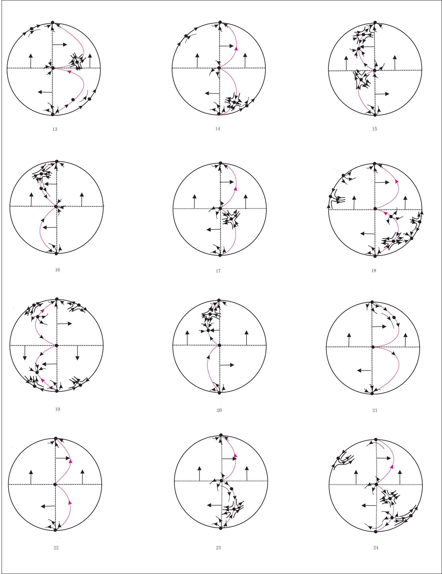
According to statement (ii) of Proposition 7 when c , d ∈ R , we get the local phase portrait from 3 to 26 of Figures 4, 5, 6, and since x ˙ ∣ x = 0 = d y and y ˙ ∣ y = 0 = ( 3 a d x 2 ) / 2 , it results from the global geometric solutions from 3 to 26 of Figures 1, 2, 3.

Figure 5

Continuation of Figure 4.

Figure 6

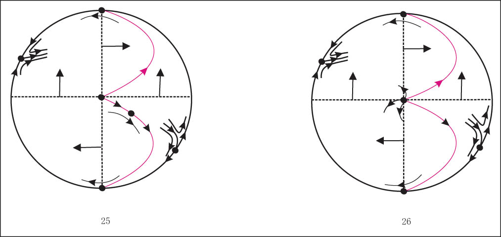
Continuation of Figure 4.

5 Conclusion

We classified the phase portraits in the Poincaré disk of two classes of quadratic systems. Our work is a continuation of the ones done in [18], in which the authors classified the phase portraits of four classes of quadratic differential systems with usual cubic invariant curves.

In this article, we analyzed two quadratic systems, the first with only one parameter, which provided six different phase portraits, and the second differential system with four parameters, and we proved by using the compactification of Poincaré that it has twenty topologically non-equivalent phase portraits.

Acknowledgements

The authors would like to express their gratitude to the managing editor and the referees for their interesting remarks and suggestions.

Funding information: The authors received no specific funding for this work.
Conflict of interest: The authors declare that there is no conflict of interest.
Data availability statement: The data sets analyzed during the current study are available from the corresponding author on reasonable request.

References

[1] F. Dumortier, J. Llibre, and J. C. Artés, Qualitative theory of planar differential systems, Springer-Verlag, Universitext (UTX), 2006, DOI: https://doi.org/10.1007/978-3-540-32902-2. 10.1007/978-3-540-32902-2Suche in Google Scholar

[2] J.C. Artés and J. Llibre, Quadratic Hamiltonian vector fields, J. Differential Equations 107 (1994), no. 1, 80–95, DOI: https://doi.org/10.1006/jdeq.1994.1004. 10.1006/jdeq.1994.1004Suche in Google Scholar

[3] J. C. Artés, J. Llibre, D. Schlomiuk, and N. Vulpe, Geometric Configurations of Singularities of Planar Polynomial Differential Systems, Birkhäuser Cham, Basel, 2021, DOI: https://doi.org/10.1007/978-3-030-50570-7. 10.1007/978-3-030-50570-7Suche in Google Scholar

[4] A. Belfar and R. Benterki, Qualitative dynamics of quadratic systems exhibiting reducible invariant algebraic curve of degree 3, Palestine J. Math. 11 (2021), no. II, 1–12, https://pjm.ppu.edu. Suche in Google Scholar

[5] A. Belfar and R. Benterki, Qualitative dynamics of quadratic polynomial differential system exhibiting an algebraic cubic first integral. Submitted (2022). Suche in Google Scholar

[6] I. V. Nikolaev and N. Vulpe, Topological classification of quadratic systems with a unique finite second order singularity with two zero eigenvalues, Bul. Acad. ŞtiinÅče Repub. Mold Mat. 11 (1993), no. 1, 3–8. Suche in Google Scholar

[7] H. Dulac, Détermination et integration d’une certaine classe d’équations différentielle ayant par point singulier un centre, Bull. Sci. Math. Sér. (2) 32 (1908), 230–252. Suche in Google Scholar

[8] W. Kapteyn, On the midpoints of integral curves of differential equations of the first degree (Dutch), Nederl. Akad. Wetensch. Verslag. Afd. Natuurk. Konikl. Nederland. 19 (1911), 1446–1457. Suche in Google Scholar

[9] W. Kapteyn, New investigations on the midpoints of integrals of differential equations of the first degree, (Dutch) Nederl. Akad. Wetensch. Verslag. Afd. Natuurk. Konikl. Nederland. 20 (1912), 1354–1365, 21 (1013), 27–33. Suche in Google Scholar

[10] N. N. Bautin, On the number of limit cycles which appear with the variation of coefficients from an equilibrium position of focus or center type, Mat. Sbornik. 30 (1952), 181–196. Amer. Math. Soc. Transl. 72 (1954), 1–19. Suche in Google Scholar

[11] V. A. Lunkevich and K. S. Sibirskii, Integrals of a general quadratic differential system in cases of a center, Differential Equations 18 (1982), no. 5, 563–568, www.mathnet.ru/eng/de/v18/i5/p786. Suche in Google Scholar

[12] W. Y. Ye and Y. Q. Ye, On the conditions of a center and general integrals of quadratic differential systems, Acta Math. Sin., Engl. Ser. 17 (2001), no. 2, 229–236, DOI: https://doi.org/10.1007/s101140100114. 10.1007/s101140100114Suche in Google Scholar

[13] J. C. Artés, J. Llibre, and N. Vulpe, Complete geometric invariant study of two classes of quadratic systems, Electron. J. Differential Equations 2012 (2012), no. 09, 1–35, http://ejde.math.txstate.edu or http://ejde.math.unt.edu. Suche in Google Scholar

[14] L. S. Lyagina, The integral curves of the equation y′=(ax2+bxy+cy2)∕(dx2+exy+fy2), (in Russian), Usp. Mat. Nauk. 42 (1951), 171–183. Suche in Google Scholar

[15] K. S. Sibirskii and N. Vulpe, Geometric classification of quadratic differential systems, Differ. Uravn. 13 (1977), 803–814. Suche in Google Scholar

[16] T. A. Newton, Two dimensional homogeneous quadratic differential systems, SIAM Review. 20 (1978), no. 1, 120–138, https://www.jstor.org/stable/2030141. 10.1137/1020007Suche in Google Scholar

[17] R. Benterki and J. Llibre, Phase portraits of quadratic polynomial differential systems having as solution some classical planar algebraic curves of degree 4, Electron. J. Differential Equations 2019 (2019), no. 15, 1–25, http://ejde.math.txstate.edu or http://ejde.math.unt.edu. Suche in Google Scholar

[18] A. Belfar and R. Benterki, Qualitative dynamics of five quadratic polynomial differential systems exhibiting five classical cubic algebraic curves, Rendiconti del Circolo Matematico di Palermo Series 2. 72 (2021), no. 1, 1–28, DOI: https://doi.org/10.1007/s12215-021-00675-x. 10.1007/s12215-021-00675-xSuche in Google Scholar

[19] J. Chavarriga, J. Giné, I. A. Garcia and E. Ribereau, Quadratic systems having third degree invariant algebraic curves, Rev. Roumaine Math. Pures Appl. 45 (2000), 93–106.Suche in Google Scholar

[20] D. A. Neumann, Classification of continuous flows on 2-manifolds, Proc. Amer. Math. Soc. 48 (1975), no. 1, 73–81, DOI: https://doi.org/10.1090/S0002-9939-1975-0356138-6. 10.1090/S0002-9939-1975-0356138-6Suche in Google Scholar

[21] L. Markus, Global structure of ordinary differential equations in the plane, Trans. Amer. Math Soc. 76 (1954), no. 1, 127–148, DOI: https://doi.org/10.2307/1990747. 10.1090/S0002-9947-1954-0060657-0Suche in Google Scholar

[22] M. M. Peixoto, Dynamical systems, Proceedings of a Symposium held at the University of Bahia, Academic Press, New York-London, A subsidiary of Harcourt Brace Jovanovich., 1973, pp. 389–420. Suche in Google Scholar

[23] W. A. Coppel, A survey of quadratic systems, J. Differential Equations 2 (1966), 293–304.10.1016/0022-0396(66)90070-2Suche in Google Scholar

Received: 2022-05-20

Revised: 2023-02-10

Accepted: 2023-03-04

Published Online: 2023-05-25

This work is licensed under the Creative Commons Attribution 4.0 International License.

Artikel in diesem Heft

https://doi.org/10.1515/dema-2022-0218

Schlagwörter für diesen Artikel

polynomial vector fields; phase portrait; invariant curve

Creative Commons

BY 4.0