New inertial forward–backward algorithm for convex minimization with applications

Kunrada Kankam; Watcharaporn Cholamjiak; Prasit Cholamjiak

doi:10.1515/dema-2022-0188

Article Open Access

New inertial forward–backward algorithm for convex minimization with applications

Kunrada Kankam , Watcharaporn Cholamjiak and Prasit Cholamjiak

Published/Copyright: February 15, 2023

Published by

Become an author with De Gruyter Brill

Author Information Explore this Subject

From the journal Demonstratio Mathematica Volume 56 Issue 1

Abstract

In this work, we present a new proximal gradient algorithm based on Tseng’s extragradient method and an inertial technique to solve the convex minimization problem in real Hilbert spaces. Using the stepsize rules, the selection of the Lipschitz constant of the gradient of functions is avoided. We then prove the weak convergence theorem and present the numerical experiments for image recovery. The comparative results show that the proposed algorithm has better efficiency than other methods.

Keywords: Tseng’s extragradient method; image recovery; inertial technique; minimization problem

MSC 2010: 65K05; 90C25; 90C30

1 Introduction and preliminaries

The forward–backward splitting (FBS) algorithm [1,2] was proposed for solving the convex minimization problem (MNP) of two objective functions in a real Hilbert space H . It is modeled as the following form:

(1.1) min { f ( k ) + g ( k ) : k ∈ H } ,

where f : H → ( − ∞ , + ∞ ] and g : H → R are two proper lower semicontinuous convex functions such that f is differentiable on H . The FBS generates an iterative sequence k 0 ∈ H and

(1.2) k n + 1 = prox λ n g ︸ backward step ( k n − λ n ∇ f ( k n ) ) ︸ forward step ,

where λ n > 0 , prox λ n g = ( I + λ n ∂ g ) − 1 is the proximal operator of g , and ∇ f is the gradient of f . The proximal operator is single-valued with full domain, and it is characterized by the relations

(1.3) k − prox λ g ( k ) λ ∈ ∂ g ( prox λ g ( k ) ) ,

for all k ∈ H and λ > 0 . The subdifferential of g is the set-valued operator ∂ g : H → 2 H , which is defined by

∂ g ( k ) = { u ∈ H ∣ g ( x ) − g ( k ) ≥ ⟨ u , x − k ⟩ , x ∈ H } .

The elements in ∂ g ( k ) are called the subgradient of g at k . The FBS includes, as a special case, the proximal point algorithm [3,4, 5,6,7, 8,9] and the gradient method [10,11,12]. Due to its wide applications, there have been modifications of (1.2) invented in the literature [13,14, 15,16].

In 2000, Tseng [17] introduced the forward–backward-forward splitting (FBFS) algorithm, also known as Tseng’s extragradient algorithm or Tseng’s method. FBFS is generated by k 0 ∈ H and

k n + 1 = prox α n g ( k n − α n ∇ f ( k n ) ) − α n ( ∇ f ( prox α n g ( k n − α n ∇ f ( k n ) ) ) − ∇ f ( k n ) ) ,

where ( α n ) is a real positive sequence. In 2005, Combettes and Wajs [1] proposed the relaxed version of FBS (FBS-CW), which is generated by k 0 = k 1 ∈ H , ε ∈ ( 0 , min { 1 , 1 / L } ) , and

(1.4) k n + 1 = k n + λ n ( prox α g ( k n − α n ∇ f ( k n ) ) − k n ) ,

where λ n ∈ [ ε , 1 ] , α n ∈ [ ε , ( 2 / L ) − ε ] , and L is the Lipschitz constant of ∇ f .

To improve the convergence of the algorithm, a popular technique is using inertial-type methods. For other inertial methods, we refer to [18,19,20, 21,22,23]. In this work, we consider the inertial forward–backward method [18,24] (IFB), which is generated by k 0 = k 1 ∈ H and

(1.5) x n = k n + θ n ( k n − k n − 1 ) , k n + 1 = prox α n g ( x n − α n ∇ f ( x n ) ) ,

where ( α n ) is a real positive sequence, θ n > 0 . Here, θ n is an extrapolation factor, and the inertial is represented by the term θ n ( k n − k n − 1 ) . In 2009, Beck and Teboulle [24] introduced a fast iterative shrinkage-thresholding algorithm method (FISTA-BT). This is similar to (1.5) with the condition α n = 1 / L and

(1.6) θ n = t n − 1 t n + 1 , where t n + 1 = 1 + 1 + 4 t n 2 2 and t 1 = 1 .

Many proximal gradient methods usually use the assumption that the gradient is Lipschitz continuous and the step size is bounded below the Lipschitz constant. This is somehow not known in practice. For this reason, Bello Cruz and Nghia [25] proposed the linesearch rule by setting α n = σ θ m n and m n is the smallest nonnegative integer such that

(1.7) α n ‖ ∇ f ( k n + 1 ) − ∇ f ( k n ) ‖ ≤ δ ‖ k n + 1 − k n ‖ .

A new version of the forward–backward method (FISTA-CN) based on (1.7) is generated by the following:

x n = k n + θ n ( k n − k n − 1 ) , y n = P Ω ( x n ) , k n + 1 = prox α n g ( y n − α n ∇ f ( y n ) ) ,

where the inertial parameter θ n is defined by (1.6). Recently, Verma and Shukla [26] introduced a new accelerated proximal gradient algorithm (NAGA), which is defined by k 0 = k 1 ∈ H and

x n = k n + θ n ( k n − k n − 1 ) , y n = ( 1 − α n ) x n + α n prox α n g ( x n − α n ∇ f ( x n ) ) , k n + 1 = prox α n g ( y n − α n ∇ f ( y n ) ) ,

where α n ∈ ( 0 , 2 / L ) and θ n is defined by (1.6).

Motivated by previous works, in this work, we are interested to introduce a new inertial proximal algorithm for solving the convex MNPs and provide a weak convergence theorem for the proposed algorithm without the Lipschitz continuity condition on the gradient. We provide numerical experiments for our algorithm to solve image recovery problems and show the efficiency of the proposed algorithms when compared with FBS-CW [1], FISTA-BT [24], FISTA-CN [25], FBFS [17], and NAGA [26].

2 Main theorem

Now, we assume that f : H → R ∪ { + ∞ } and g : H → R ∪ { + ∞ } are proper, lower semicontinuous, and convex functions, f is uniformly continuous on bounded sets, and ∇ f is bounded on bounded sets. The following is our algorithm.

Algorithm 2.1

The inertial modified FBS (IMFBS) algorithm.

Initialization: Given σ , θ , μ 1 > 0 , δ ∈ 0 , 1 2 , and ρ ∈ ( 0 , 1 ) .

Iterative step: Let k 0 = k 1 ∈ H and calculate k n + 1 as follows:

Step 1. Compute the inertial step:

x n = k n + θ n ( k n − k n − 1 ) ,

where ( θ n ) is a positive sequence.

Step 2. Compute the forward–backward step:

p n = prox α n g ( x n − α n ∇ f ( x n ) ) ,

where α n = σ θ m n and m n is the smallest nonnegative number such that:

(2.1) α n ‖ ∇ f ( p n ) − ∇ f ( x n ) ‖ ≤ δ ‖ p n − x n ‖ .

Step 3. Compute the forward–backward step:

r n = prox μ n g ( p n − μ n ∇ f ( p n ) ) .

Step 4. Compute the k n + 1 step:

k n + 1 = r n + μ n ( ∇ f ( p n ) − ∇ f ( r n ) )

and update

(2.2) μ n + 1 = min ρ ‖ p n − r n ‖ ‖ ∇ f ( p n ) − ∇ f ( r n ) ‖ , μ n if ‖ ∇ f ( p n ) − ∇ f ( r n ) ‖ ≠ 0 ; μ n otherwise .

Set n ≔ n + 1 and return to Step 1.

Remark 2.2

By [25], we know that the Linesearch (2.1) stops after finitely many steps.
By (2.2), we see that the sequence ( μ n ) is nonincreasing.

Theorem 2.3

Suppose that α n ≥ α for some α > 0 , θ n ≥ 0 , and ∑ n = 1 ∞ θ n < + ∞ . Then, the sequence ( k n ) generated by Algorithm 2.1 converges weakly to a minimizer of f + g .

Proof

Let k ∗ ∈ argmin ( f + g ) . Following the definition of r n , we have

(2.3) p n − r n − μ n ∇ f ( p n ) ∈ μ n ∂ g ( r n ) .

By definition of k n + 1 , we see that

(2.4) μ n ∇ f ( p n ) = k n + 1 − r n + μ n ∇ f ( r n ) .

From (2.3) and (2.4), we have

(2.5) p n − k n + 1 − μ n ∇ f ( r n ) ∈ μ n ∂ g ( r n ) .

Since k ∗ ∈ argmin ( f + g ) , we obtain − μ n ∇ f ( k ∗ ) ∈ μ n ∂ g ( k ∗ ) . Thus, by relation (2.5) and the monotonicity of ∂ g , we have

⟨ p n − k n + 1 − μ n ( ∇ f ( r n ) − ∇ f ( k ∗ ) ) , r n − k ∗ ⟩ ≥ 0 .

This, together with the monotonicity of ∇ f , implies that

⟨ p n − k n + 1 , r n − k ∗ ⟩ ≥ 0 .

Hence, we have

(2.6) ⟨ p n − k n + 1 , r n − k n + 1 ⟩ + ⟨ p n − k n + 1 , k n + 1 − k ∗ ⟩ ≥ 0 .

We know that ‖ x ± y ‖ 2 = ‖ x ‖ 2 ± 2 ⟨ x , y ⟩ + ‖ y ‖ 2 . So by (2.6), we obtain

1 2 [ ‖ p n − k n + 1 ‖ 2 + ‖ k n + 1 − r n ‖ 2 − ‖ p n − r n ‖ 2 ] + 1 2 [ ‖ p n − k ∗ ‖ 2 − ‖ p n − k n + 1 ‖ 2 − ‖ k n + 1 − k ∗ ‖ 2 ] ≥ 0 .

It implies that

(2.7) ‖ k n + 1 − k ∗ ‖ 2 ≤ ‖ p n − k ∗ ‖ 2 + ‖ k n + 1 − r n ‖ 2 − ‖ p n − r n ‖ 2 .

By definition of k n + 1 and (2.2), we have

(2.8) ‖ k n + 1 − r n ‖ 2 ≤ ‖ r n + μ n ( ∇ f ( p n ) − ∇ f ( r n ) ) − r n ‖ 2 = μ n 2 ‖ ∇ f ( p n ) − ∇ f ( r n ) ‖ 2 .

Note that

μ n + 1 = min ρ ‖ p n − r n ‖ ‖ ∇ f ( p n ) − ∇ f ( r n ) ‖ , μ n ≤ ρ ‖ p n − r n ‖ ‖ ∇ f ( p n ) − ∇ f ( r n ) ‖ .

It follows that

(2.9) ‖ ∇ f ( p n ) − ∇ f ( r n ) ‖ ≤ ρ μ n + 1 ‖ p n − r n ‖ .

Combining (2.8) and (2.9), we have

(2.10) ‖ k n + 1 − r n ‖ 2 ≤ ρ 2 μ n 2 μ n + 1 2 ‖ p n − r n ‖ 2 .

By definition of p n , we have

x n − p n α n − ∇ f ( x n ) ∈ ∂ g ( p n ) .

By the convexity of g , we obtain

(2.11) g ( k ∗ ) − g ( p n ) ≥ x n − p n α n − ∇ f ( x n ) , k ∗ − p n .

By the convexity of f , we see that

(2.12) f ( k ∗ ) − f ( x n ) ≥ ⟨ ∇ f ( x n ) , k ∗ − x n ⟩ .

Combining (2.1), (2.11), and (2.12), we have

(2.13) ( f + g ) ( k ∗ ) ≥ g ( p n ) + f ( x n ) + x n − p n α n − ∇ f ( x n ) , k ∗ − p n + ⟨ ∇ f ( x n ) , k ∗ − x n ⟩ = g ( p n ) + f ( x n ) + 1 α n ⟨ x n − p n , k ∗ − p n ⟩ + ⟨ ∇ f ( x n ) − ∇ f ( p n ) , p n − x n ⟩ + ⟨ ∇ f ( p n ) , p n − x n ⟩ ≥ g ( p n ) + f ( x n ) + 1 α n ⟨ x n − p n , k ∗ − p n ⟩ − ‖ ∇ f ( x n ) − ∇ f ( p n ) ‖ ‖ p n − x n ‖ + ⟨ ∇ f ( p n ) , p n − x n ⟩ ≥ g ( p n ) + f ( x n ) + 1 α n ⟨ x n − p n , k ∗ − p n ⟩ − δ α n ‖ p n − x n ‖ 2 + ⟨ ∇ f ( p n ) , p n − x n ⟩ .

By (2.13) and the convexity of f , we obtain

(2.14) 1 α n ⟨ x n − p n , p n − k ∗ ⟩ ≥ g ( p n ) + f ( x n ) − ( f + g ) ( k ∗ ) − δ α n ‖ p n − x n ‖ 2 + f ( p n ) − f ( x n ) = ( f + g ) ( p n ) − ( f + g ) ( k ∗ ) − δ α n ‖ p n − x n ‖ 2 .

We see that ‖ x n − k ∗ ‖ 2 = ‖ x n − p n ‖ 2 + 2 ⟨ x n − p n , p n − k ∗ ⟩ + ‖ p n − k ∗ ‖ 2 . By (2.14), we have

‖ x n − k ∗ ‖ 2 − ‖ x n − p n ‖ 2 − ‖ p n − k ∗ ‖ 2 ≥ 2 α n [ ( f + g ) ( p n ) − ( f + g ) ( k ∗ ) ] − 2 δ ‖ p n − x n ‖ 2 .

It implies that

(2.15) ‖ p n − k ∗ ‖ 2 ≤ ‖ x n − k ∗ ‖ 2 − ( 1 − 2 δ ) ‖ x n − p n ‖ 2 − 2 α n [ ( f + g ) ( p n ) − ( f + g ) ( k ∗ ) ] .

Hence, from (2.7), (2.10), and (2.15), we obtain

(2.16) ‖ k n + 1 − k ∗ ‖ 2 ≤ ‖ x n − k ∗ ‖ 2 − ( 1 − 2 δ ) ‖ x n − p n ‖ 2 − 2 α n [ ( f + g ) ( p n ) − ( f + g ) ( k ∗ ) ] − 1 − ρ 2 μ n 2 μ n + 1 2 ‖ p n − r n ‖ 2 .

Now, we will show that ( k n ) is bounded. From (2.16) and by definition of ( x n ) , we have

‖ k n + 1 − k ∗ ‖ ≤ ‖ x n − k ∗ ‖ = ‖ k n + θ n ( k n − k n − 1 ) − k ∗ ‖ ≤ ‖ k n − k ∗ ‖ + θ n ( ‖ k n − k ∗ ‖ + ‖ k n − 1 − k ∗ ‖ ) .

This shows that

‖ k n + 1 − k ∗ ‖ ≤ ( 1 + θ n ) ‖ k n − k ∗ ‖ + θ n ‖ k n − 1 − k ∗ ‖ .

By Lemma 5 in [27], we conclude that

‖ k n + 1 − k ∗ ‖ ≤ K ⋅ ∏ j = 1 n ( 1 + 2 θ j ) ,

where K = max { ‖ k 1 − k ∗ ‖ , ‖ k 2 − k ∗ ‖ } . Since ∑ n = 1 ∞ θ n < + ∞ , we have ( k n ) , which is bounded. From (2.16), we have

(2.17) ‖ k n + 1 − k ∗ ‖ 2 ≤ ‖ k n + θ n ( k n − k n − 1 ) − k ∗ ‖ 2 − ( 1 − 2 δ ) ‖ x n − p n ‖ 2 − 2 α n [ ( f + g ) ( p n ) − ( f + g ) ( k ∗ ) ] − 1 − ρ 2 μ n 2 μ n + 1 2 ‖ p n − r n ‖ 2 = ‖ k n − k ∗ ‖ 2 + 2 θ n ‖ k n − k ∗ ‖ ‖ k n − k n − 1 ‖ + θ n 2 ‖ k n − k n − 1 ‖ 2 − ( 1 − 2 δ ) ‖ x n − p n ‖ 2 − 2 α n [ ( f + g ) ( p n ) − ( f + g ) ( k ∗ ) ] − 1 − ρ 2 μ n 2 μ n + 1 2 ‖ p n − r n ‖ 2 .

Since lim n → ∞ θ n ‖ k n − k n − 1 ‖ = 0 , lim n → ∞ ‖ k n − k ∗ ‖ exists, and 1 − 2 δ > 0 , we have

lim n → ∞ ‖ x n − p n ‖ = 0 .

By definition of x n , we have lim n → ∞ ‖ x n − k n ‖ = 0 . Then,

‖ p n − k n ‖ ≤ ‖ x n − p n ‖ + ‖ x n − k n ‖ → 0 as n → ∞ .

Since lim n → ∞ 1 − μ n 2 ρ 2 μ n + 1 2 = 1 − ρ 2 > 0 , we have lim n → ∞ ‖ p n − r n ‖ = 0 . So, we have

‖ r n − k n ‖ ≤ ‖ p n − r n ‖ + ‖ p n − k n ‖ → 0 as n → ∞ .

Since the sequence ( k n ) is bounded, assume that k ∞ is a weak limit point of ( k n ) , i.e., there is a subsequence ( k n i ) of ( k n ) such that k n i ⇀ k ∞ . Since lim i → ∞ ‖ r n i − k n i ‖ = 0 , we also obtain r n i ⇀ k ∞ as i → ∞ . Since ( p n i ) is bounded, lim i → ∞ ‖ p n i − r n i ‖ = 0 , and ∇ f is uniformly continuous on H , we have

lim i → ∞ ‖ ∇ f ( p n i ) − ∇ f ( r n i ) ‖ = 0 .

From (1.3), we obtain

p n i − r n i α n i − ∇ f ( p n i ) = p n i − prox α n i g ( p n i − α n i ∇ f ( p n i ) ) − α n i ∇ f ( p n i ) α n i ∈ ∂ g ( p n i − α n i ∇ f ( p n i ) ) .

It follows that

p n i − r n i α n i + ∇ f ( r n i ) − ∇ f ( p n i ) ∈ ∇ f ( r n i ) + ∂ g ( r n i ) ⊆ ∂ ( f + g ) ( r n i ) .

By passing i → ∞ and using Fact 2.2 in [25], we have 0 ∈ ∇ f ( k ∞ ) + ∂ g ( k ∞ ) . Thus, k ∞ ∈ argmin ( f + g ) . Hence, by Theorem 5.5 in [28], we can conclude that ( k n ) converges weakly to a point in argmin ( f + g ) . We thus complete the proof.□

3 Numerical experiments

In this section, we apply Algorithm 2.1 to solve the image restoration problem and compare the efficiency of FBS-CW [1], FISTA-BT [24], FISTA-CN [25], FBFS [17], and NAGA [26]. The numerical experiments are performed by Matlab 2020b on a 64-bit MacBook Pro Chip Apple M1 and 8 GB of RAM.

The image restoration problem can be modeled as follows:

(3.1) b = A k + w ,

where b ∈ R m × 1 is the observed image, A ∈ R m × n is the blurring matrix, k ∈ R n × 1 is an original image, and w is additive noise. To solve problem (3.1), we aim to approximate the original image by transforming (3.1) to the following LASSO problem [29]:

(3.2) min k 1 2 ‖ b − A k ‖ 2 2 + λ ‖ k ‖ 1 ,

where ‖ ⋅ ‖ 1 is ℓ 1 -norm. In general, (3.2) can be formulated in a general form by estimating the minimizer of the sum of two functions when f ( k ) = 1 2 ‖ b − A k ‖ 2 2 and g ( k ) = λ ‖ k ‖ 1 .

To evaluate the quality of the restored images, we use the peak signal-to-noise ratio (PSNR) [30] and the structural similarity index (SSIM) [31], which are defined as follows:

(3.3) PSNR = 20 log ‖ k ‖ F ‖ k − k r ‖ F

and

(3.4) SSIM = ( 2 u k u k r + c 1 ) ( 2 σ k k r + c 2 ) ( u k 2 + u k r 2 + c 1 ) ( σ x 2 + σ k r 2 + c 2 ) ,

where k is the original image, k r is the restored image, u k and u k r are the mean values of the original image k and restored image k r , respectively, σ k 2 and σ k r 2 are the variances, σ k k r 2 is the covariance of two images, c 1 = ( K 1 L ) 2 and c 2 = ( K 2 L ) 2 with K 1 = 0.01 and K 2 = 0.03 , and L is the dynamic range of pixel values. SSIM ranges from 0 to 1, and 1 means perfect recovery.

All parameters are chosen as in Table 1. The initial point k 0 = k 1 are vectors of ones with the size of the original images for all algorithms. The parameter θ n of FISTA-BT, FISTA-CN, and NAGA is defined as (1.6). We also set θ n in Algorithm 2.1 (IMFBS) by

θ n = t n − 1 t n + 1 where t n + 1 = 1 + 1 + 4 t n 2 2 , if 1 ≤ n ≤ M ; 1 n 2 , otherwise .

Table 1

Chosen parameters of each algorithm

Algorithms	Chosen parameters
	t 1 = 1	α n = 1 / 2 ‖ A ‖ 2	λ n = 0.5	δ = θ = 0.4	σ = 0.2	ρ = μ 1 = 0.4
FBS-CW		√	√
FISTA-BT	√	√
FISTA-CN	√			√	√
NAGA	√	√
FBFS		√
IMFBS	√			√	√	√

The original images and three different blurring matrices types for the original images of sizes 448 × 298 and 240 × 320 are shown in Figures 1 and 2, respectively.

$Figure 1 The original image size 448 × 298 448\times 298 (Fig(A)) and the deblurred RGB images by out-of-focus blur matrices with radius 6 (BM-1.1), Gaussian blur with standard deviation 7 of the filter size [ 5 × 5 ] \left[5\times 5] (BM-1.2), and the deblurred images by motion blur specified with the motion length of 11 pixels and motion orientation 23 (BM-1.3), respectively.$

Figure 1

The original image size 448 × 298 (Fig(A)) and the deblurred RGB images by out-of-focus blur matrices with radius 6 (BM-1.1), Gaussian blur with standard deviation 7 of the filter size [ 5 × 5 ] (BM-1.2), and the deblurred images by motion blur specified with the motion length of 11 pixels and motion orientation 23 (BM-1.3), respectively.

$Figure 2 The original image size 240 × 320 240\times 320 (Fig(A)) and the deblurred RGB image by out-of-focus blur matrices with radius 6 (BM-1.1), Gaussian blur with standard deviation 7 of the filter size [ 5 × 5 ] \left[5\times 5] (BM-2.2), and the deblurred image by motion blur specified with the motion length of 11 pixels and motion orientation 23 (BM-2.3), respectively.$

Figure 2

The original image size 240 × 320 (Fig(A)) and the deblurred RGB image by out-of-focus blur matrices with radius 6 (BM-1.1), Gaussian blur with standard deviation 7 of the filter size [ 5 × 5 ] (BM-2.2), and the deblurred image by motion blur specified with the motion length of 11 pixels and motion orientation 23 (BM-2.3), respectively.

The results of the deblurred images with M iterations for each algorithm are shown in Tables 2 and 3. We provide some experiments of recovered images of Fig(A) for two cases and one case for Fig(B) to illustrate the convergence behavior of all algorithms in Figures 3, 4, and 5.

Table 2

The results of deblurred images for each algorithm

Fig(A)	M	Algorithms	Blurred type
			BM-1.1		BM-1.2		BM-1.3
			PSNR	SSIM	PSNR	SSIM	PSNR	SSIM
The original image size 448 × 298	500	FBS-CW	25.8764	0.7715	29.0112	0.8899	31.2942	0.9242
		FISTA-BT	35.5477	0.9446	38.3302	0.9621	40.5405	0.9835
		FISTA-CN	36.5491	0.9543	39.5388	0.9705	41.8671	0.9871
		NAGA	36.2057	0.9514	39.1270	0.9678	41.4341	0.9859
		FBFS	24.2054	0.7072	27.5600	0.8583	29.8552	0.8996
		IMFBS	38.7966	0.9702	41.6765	0.9816	44.6781	0.9930
	1,000	FBS-CW	26.1910	0.7837	29.2922	0.8957	31.5644	0.9286
		FISTA-BT	37.0305	0.9586	39.6679	0.9715	41.7964	0.9883
		FISTA-CN	38.1887	0.9664	40.9419	0.9780	43.1783	0.9911
		NAGA	37.7800	0.9641	40.5485	0.9759	42.6821	0.9901
		FBFS	24.6732	0.7225	27.8260	0.8662	30.1126	0.9053
		IMFBS	40.5491	0.9782	43.2354	0.9868	45.9856	0.9950
	1,500	FBS-CW	26.4418	0.7923	29.5205	0.8996	31.7869	0.9318
		FISTA-BT	38.0757	0.9664	40.6216	0.9765	42.6318	0.9906
		FISTA-CN	39.2981	0.9726	41.9730	0.9833	44.0774	0.9330
		NAGA	38.8771	0.9708	41.5473	0.9813	43.5755	0.9923
		FBFS	24.8915	0.7331	28.0377	0.8717	30.3250	0.9094
		IMFBS	41.7181	0.9828	44.4942	0.9901	47.3108	0.9964

Table 3

The results of deblurred images for each algorithm

Fig(B)	M	Algorithms	Blurred type
			BM-2.1		BM-2.2		BM-2.3
			PSNR	SSIM	PSNR	SSIM	PSNR	SSIM
The original image size 240 × 320	500	FBS-CW	28.1063	0.8764	33.3164	0.9479	32.8894	0.9503
		FISTA-BT	38.4144	0.9733	42.9090	0.9888	42.9989	0.9911
		FISTA-CN	39.3158	0.9779	43.9720	0.9910	44.3774	0.9932
		NAGA	39.0548	0.9767	43.6322	0.9904	43.9016	0.9926
		FBFS	26.7863	0.8427	31.5921	0.9344	31.3430	0.9354
		IMFBS	41.2504	0.9843	46.2374	0.9945	46.6263	0.9958
	1,000	FBS-CW	28.3151	0.8818	33.5886	0.9507	33.1323	0.9530
		FISTA-BT	39.1638	0.9772	43.9748	0.9912	44.0517	0.9931
		FISTA-CN	40.1671	0.9813	45.1091	0.9929	45.4008	0.9948
		NAGA	39.9064	0.9804	44.7171	0.9923	45.1169	0.9945
		FBFS	26.9618	0.8486	31.8549	0.9378	31.5693	0.9388
		IMFBS	42.2498	0.9874	47.3408	0.9957	47.6728	0.9968
	1,500	FBS-CW	28.5033	0.8862	33.8154	0.9526	33.3404	0.9549
		FISTA-BT	39.7800	0.9800	44.7409	0.9925	44.9116	0.9943
		FISTA-CN	40.8390	0.9836	45.9122	0.9941	46.2742	0.9957
		NAGA	40.4829	0.9825	45.5109	0.9936	45.8330	0.9953
		FBFS	27.1200	0.8534	32.0793	0.9402	31.7652	0.9412
		IMFBS	43.0213	0.9891	48.0766	0.9963	48.6282	0.9974

Figure 3

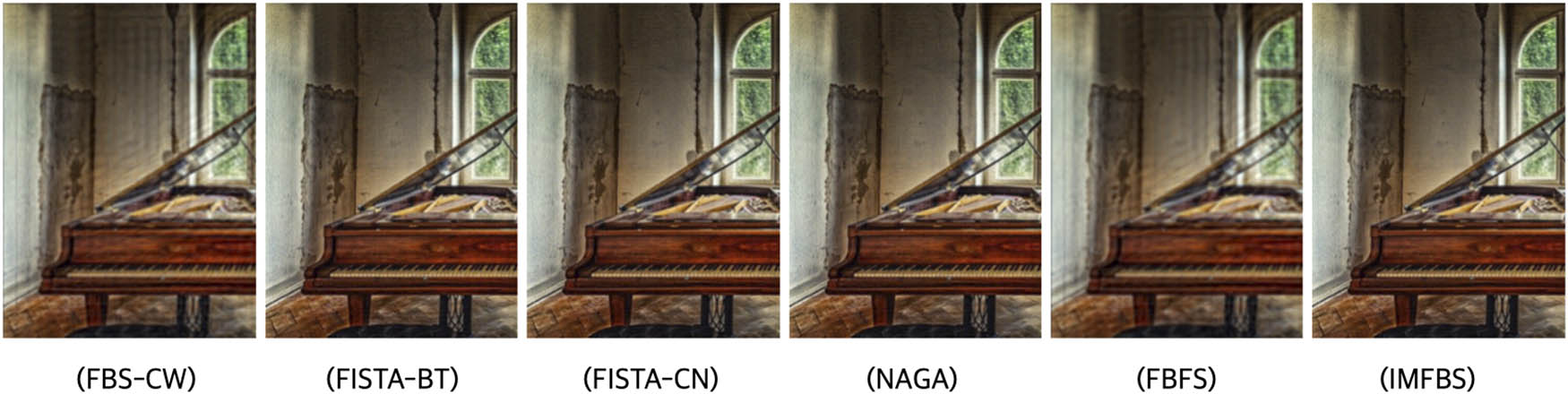
The restored images by BM-1.1 for FBS-CW (PSNR:26.07923, SSIM:0.7923), FISTA-BT (PSNR:38.9664, SSIM:0.9664), FISTA-CN (PSNR:39.2981, SSIM:0.9726), NAGA (PSNR:38.8771 SSIM:0.9708), FBFS (PSNR:24.8915 SSIM:0.7331), and IMFBS (PSNR:41.7181, SSIM:0.9828), respectively.

Figure 4

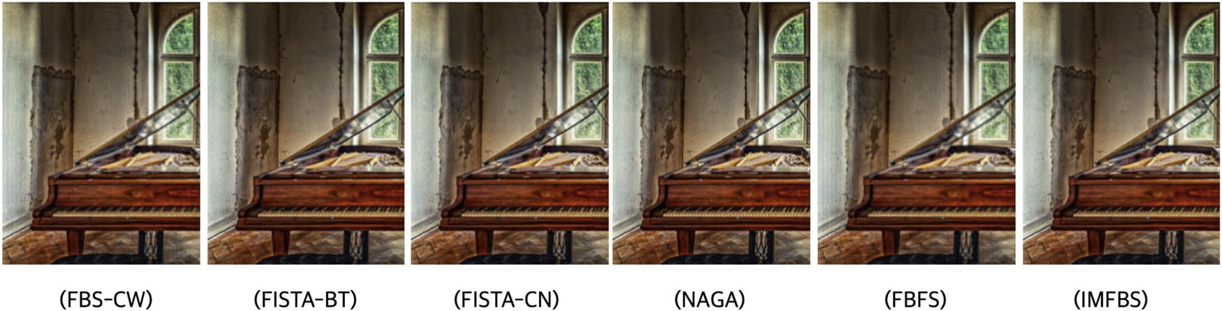
The restored images by BM-1.2 for FBS-CW (PSNR:29.5205, SSIM:0.8996), FISTA-BT (PSNR:40.6212, SSIM:0.9765), FISTA-CN (PSNR:41.9730, SSIM:0.9833), NAGA (PSNR:41.5473, SSIM:0.9813), FBFS (PSNR:28.0377, SSIM:0.8717), and IMFBS (PSNR:44.4942, SSIM:0.9901), respectively.

Figure 5

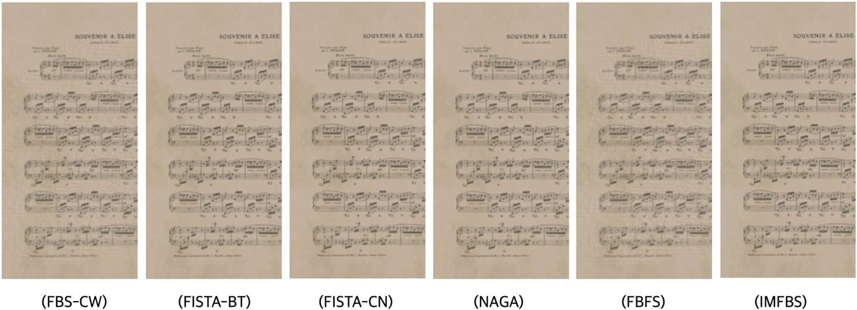
The restored images by BM-2.3 for FBS-CW (PSNR:33.3404, SSIM:0.9549), FISTA-BT (PSNR:44.9116, SSIM:0.9943), FISTA-CN (PSNR:46.2742, SSIM:0.9957), NAGA (PSNR:45.8330, SSIM:0.9953), FBFS (PSNR:31.7652, SSIM:0.9412), and IMFBS (PSNR:48.6282, SSIM:0.9974), respectively.

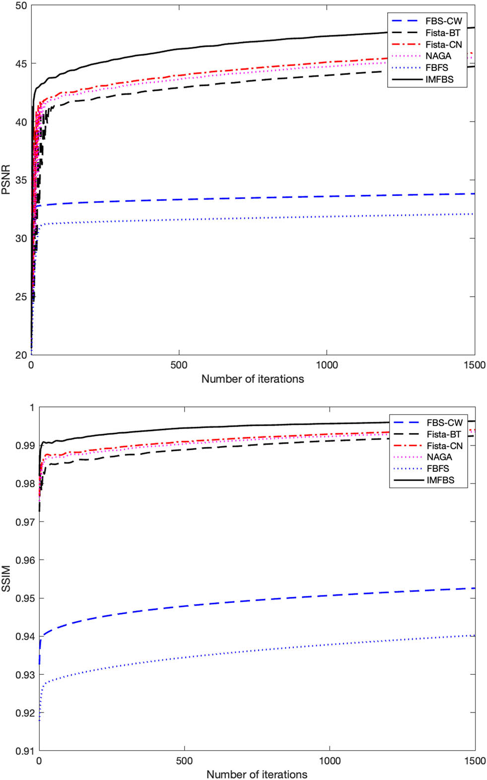
In Figures 6, 7, and 8, we plot the number of iterations versus the PSNR [30] and the SSIM [31].

Figure 6

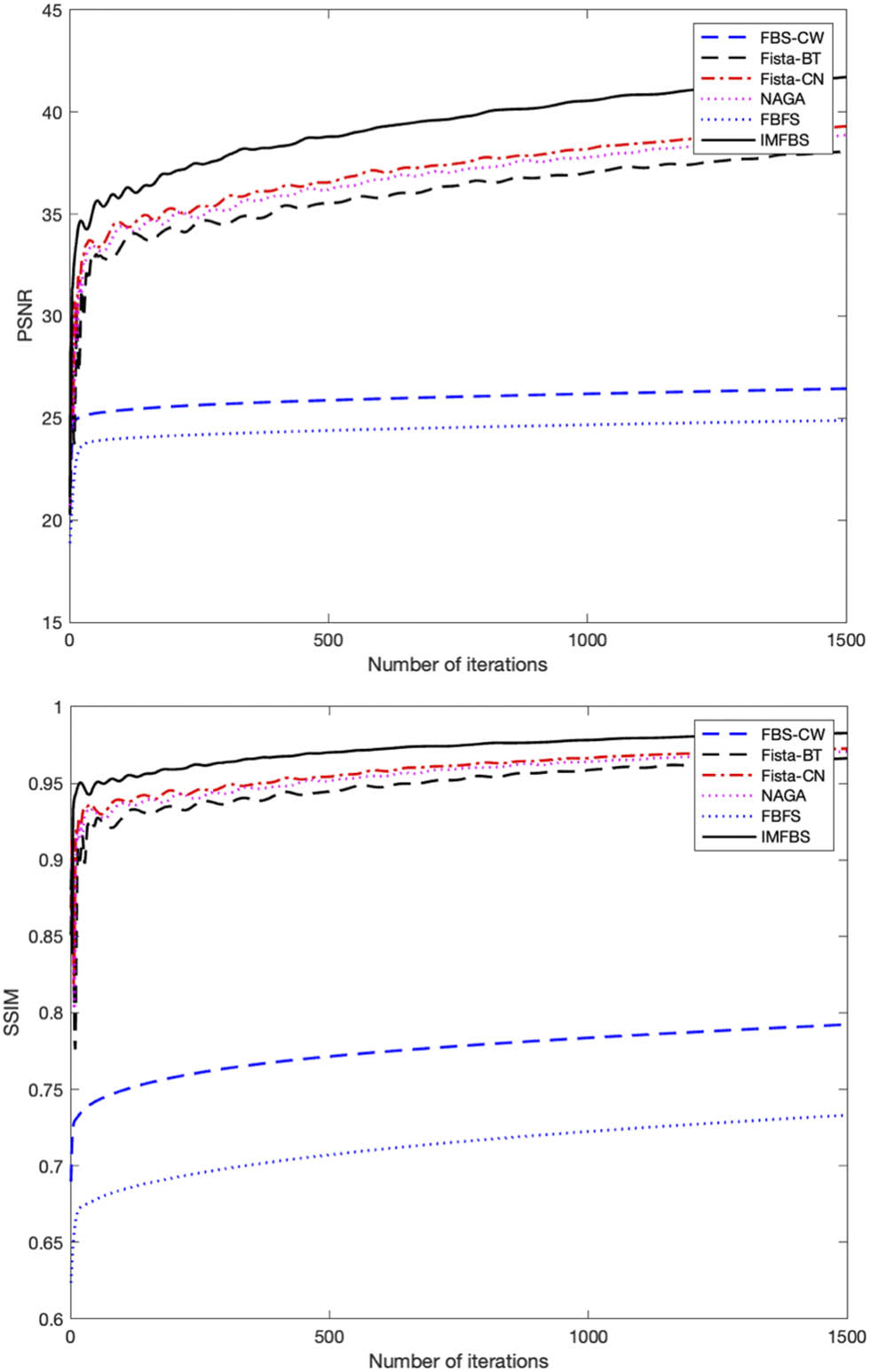
Graphs of PSNR and SSIM for FIG(A) by out of focusing, respectively.

Figure 7

Graphs of PSNR and SSIM for FIG(A) by Gaussian blur matrices, respectively.

Figure 8

Graphs of PSNR and SSIM for Fig(B) by motion blurring, respectively.

4 Conclusion

In this work, we have introduced a new inertial proximal gradient algorithm for solving the convex MNPs and have proved a weak convergence theorem without the Lipschitz continuity conditions on the gradient of functions. We provided some numerical experiments and applied our algorithm to the image recovery problem. We also compared our algorithm with FBS-CW [1], FISTA-BT [24], FISTA-CN [25], FBFS [17], and NAGA [26]. It was shown that our algorithm has better efficiency than other algorithms in terms of PSNR and SSIM for all blurred types.

Acknowledgement

The authors sincerely thank the anonymous reviewers for their careful reading, constructive comments, and suggestions for some related references that improved the manuscript substantially.

Funding information: This work was supported by the National Research Council of Thailand under grant no. N41A640094 and the Thailand Science Research and Innovation Fund and the University of Phayao under the project FF66-UoE.
Author contributions: The authors conceived the study, participated in its design and coordination, drafted the manuscript, participated in the sequence alignment, and read and approved the final manuscript.
Conflict of interest: The authors declare that they have no competing interests.
Data availability statement: Data sharing is not applicable to this article as no datasets were generated or analyzed during this study.

References

[1] P. L. Combettes and V. R. Wajs, Signal recovery by proximal forward–backward splitting, Multiscale Model. Simul. 4 (2005), 1168–1200, DOI: https://doi.org/10.1137/050626090. 10.1137/050626090Search in Google Scholar

[2] P. L. Lions and B. Mercier, Splitting algorithms for the sum of two nonlinear operators, SIAM J. Numer. Anal. 16 (1979), 964–979, DOI: https://doi.org/10.1137/0716071. 10.1137/0716071Search in Google Scholar

[3] S. Khatoon, W. Cholamjiak, and I. Uddin, A modified proximal point algorithm involving nearly asymptotically quasi-nonexpansive mappings, J. Inequal. Appl. 2021 (2021), 1–20, DOI: https://doi.org/10.1186/s13660-021-02618-7. 10.1186/s13660-021-02618-7Search in Google Scholar

[4] S. Khatoon, I. Uddin, and M. Basarir, A modified proximal point algorithm for a nearly asymptotically quasi-nonexpansive mapping with an application, Comput. Appl. Math. 40 (2021), 1–19, DOI: https://doi.org/10.1007/s40314-021-01646-9. 10.1007/s40314-021-01646-9Search in Google Scholar

[5] C. Khunpanuk, C. Garodia, I. Uddin, and N. Pakkaranang, On a proximal point algorithm for solving common fixed point problems and convex minimization problems in Geodesic spaces with positive curvature, AIMS Math. 7 (2022), 9509–9523, DOI: https://doi.org/10.3934/math.2022529. 10.3934/math.2022529Search in Google Scholar

[6] C. Garodia, I. Uddin, and D. Baleanu, On constrained minimization, variational inequality and split feasibility problem via new iteration scheme in Banach spaces, Bull. Iran. Math. Soc. 48 (2022), 1493–1512, DOI: https://doi.org/10.1007/s41980-021-00596-6. 10.1007/s41980-021-00596-6Search in Google Scholar

[7] T. Kajimura and Y. Kimura, The proximal point algorithm in complete geodesic spaces with negative curvature, Adv. Theory Nonlinear Anal. Appl. 3 (2019), 192–200, DOI: https://doi.org/10.31197/atnaa.573972. 10.31197/atnaa.573972Search in Google Scholar

[8] M. A. Hajji, Forward-backward alternating parallel shooting method for multi-layer boundary value problems, Adv. Theory Nonlinear Anal. Appl. 4 (2020), 432–442, DOI: https://doi.org/10.31197/atnaa.753561. 10.31197/atnaa.753561Search in Google Scholar

[9] A. N. Iusem, B. F. Svaiter, and M. Teboulle, Entropy-like proximal methods in convex programming, Math. Oper. Res. 19 (1994), 790–814, DOI: https://doi.org/10.1287/moor.19.4.790. 10.1287/moor.19.4.790Search in Google Scholar

[10] J. C. Dunn, Convexity, monotonicity, and gradient processes in Hilbert space, J. Math. Anal. Appl. 53 (1976), 145–158, DOI: https://doi.org/10.1016/0022-247X(76)90152-9. 10.1016/0022-247X(76)90152-9Search in Google Scholar

[11] C. Wang and N. Xiu, Convergence of the gradient projection method for generalized convex minimization, Comput. Optim. Appl. 16 (2000), 111–120, DOI: https://doi.org/10.1023/A:1008714607737. 10.1023/A:1008714607737Search in Google Scholar

[12] H. K. Xu, Averaged mappings and the gradient-projection algorithm, J. Optim. Theory Appl. 150 (2011), 360–378, DOI: https://doi.org/10.1007/s10957-011-9837-z. 10.1007/s10957-011-9837-zSearch in Google Scholar

[13] K. Kankam, N. Pholasa, and P. Cholamjiak, On convergence and complexity of the modified forward-Řbackward method involving new linesearches for convex minimization. Math. Methods Appl. Sci. 42 (2019), 1352–1362, DOI: https://doi.org/10.1002/mma.5420. 10.1002/mma.5420Search in Google Scholar

[14] S. Suantai, M. A. Noor, K. Kankam, and P. Cholamjiak, Novel forward–backward algorithms for optimization and applications to compressive sensing and image inpainting, Adv. Difference Equ. 2021 (2021), 1–22, DOI: https://doi.org/10.1186/s13662-021-03422-9. 10.1186/s13662-021-03422-9Search in Google Scholar

[15] K. Kankam, N. Pholasa, and P. Cholamjiak, Hybrid forward–backward algorithms using linesearch rule for minimization problem, Thai J. Math. 17 (2019), 607–625. Search in Google Scholar

[16] K. Kankam and P. Cholamjiak, Strong convergence of the forward–backward splitting algorithms via linesearches in Hilbert spaces, Appl. Anal. 2021 (2021), 1–20, DOI: https://doi.org/10.1080/00036811.2021.1986021. 10.1080/00036811.2021.1986021Search in Google Scholar

[17] P. Tseng, A modified forward–backward splitting method for maximal monotone mappings, SIAM J. Control Optim. 38 (2000), 431–446, DOI: https://doi.org/10.1137/S0363012998338806. 10.1137/S0363012998338806Search in Google Scholar

[18] H. Attouch and J. Peypouquet, The rate of convergence of Nesterov’s accelerated forward–backward method is actually faster than 1∕k2, SIAM J. Control Optim. 26 (2016), 1824–1834, DOI: https://doi.org/10.1137/15M1046095. 10.1137/15M1046095Search in Google Scholar

[19] A. Moudafi and M. Oliny, Convergence of a splitting inertial proximal method for monotone operators, J. Comput. Appl. Math. 155 (2003), 447–454, DOI: https://doi.org/10.1016/S0377-0427(02)00906-8. 10.1016/S0377-0427(02)00906-8Search in Google Scholar

[20] Y. E. Nesterov, A method for solving the convex programming problem with convergence rate O(1∕k2), Dokl. Akad. Nauk SSR. 269 (1983), 543–547. Search in Google Scholar

[21] B. T. Polyak, Some methods of speeding up the convergence of iteration methods, USSR Comput. Math. Math. Phys. 4 (1964), 1–17, DOI: https://doi.org/10.1016/0041-5553(64)90137-5. 10.1016/0041-5553(64)90137-5Search in Google Scholar

[22] F. Akutsah, A. A. Mebawondu, G. C. Ugwunnadi, and O. K. Narain, Inertial extrapolation method with regularization for solving monotone bilevel variation inequalities and fixed point problems, J. Nonlinear Funct. Anal. 2022 (2022), 5, DOI: https://doi.org/10.23952/jnfa.2022.5. 10.23952/jnfa.2022.5Search in Google Scholar

[23] L. Liu, S. Y. Cho, and J. C. Yao, Convergence analysis of an inertial Tseng’s extragradient algorithm for solving pseudomonotone variational inequalities and applications, J. Nonlinear Var. Anal. 5 (2021), 627–644. Search in Google Scholar

[24] A. Beck and M. Teboulle, A fast iterative shrinkage-thresholding algorithm for linear inverse problems, SIAM J. Imaging Sci. 2 (2009), 183–202, DOI: https://doi.org/10.1137/080716542. 10.1137/080716542Search in Google Scholar

[25] J. Y. Bello Cruz and T. T. Nghia, On the convergence of the forward–backward splitting method with linesearches, Optim. Methods Softw. 31 (2016), 1209–1238, DOI: https://doi.org/10.1080/10556788.2016.1214959. 10.1080/10556788.2016.1214959Search in Google Scholar

[26] M. Verma and K. K. Shukla, A new accelerated proximal gradient technique for regularized multitask learning framework, Pattern Recognit. Lett. 95 (2017), 98–103, DOI: https://doi.org/10.1016/j.patrec.2017.06.013. 10.1016/j.patrec.2017.06.013Search in Google Scholar

[27] A. Hanjing and S. Suantai, A fast image restoration algorithm based on a fixed point and optimization method, Mathematics, 8 (2020), 378, DOI: https://doi.org/10.3390/math8030378. 10.3390/math8030378Search in Google Scholar

[28] H. H. Bauschke and P. L. Combettes, Convex Analysis and Monotone Operator Theory in Hilbert Spaces, Springer, New York, 2011. 10.1007/978-1-4419-9467-7Search in Google Scholar

[29] R. Tibshirani, Regression shrinkage and selection via the lasso, J. R. Stat. Soc. Series B. Stat. Methodol. 58 (1996), 267–288, DOI: https://doi.org/10.1111/j.2517-6161.1996.tb02080.x. 10.1111/j.2517-6161.1996.tb02080.xSearch in Google Scholar

[30] K. H. Thung and P. Raveendran, A survey of image quality measures. In 2009 International Conference for Technical Postgraduates (TECHPOS), IEEE; 2009, December. p. 1–4. 10.1109/TECHPOS.2009.5412098Search in Google Scholar

[31] Z. Wang, A. C. Bovik, and E. P. Simoncelli, Image quality assessment: from error visibility to structural similarity, IEEE Trans. Image Process. 13 (2004), 600–612, DOI: https://doi.org/10.1109/TIP.2003.819861. 10.1109/TIP.2003.819861Search in Google Scholar PubMed

Received: 2022-07-22

Revised: 2022-10-25

Accepted: 2022-11-27

Published Online: 2023-02-15

This work is licensed under the Creative Commons Attribution 4.0 International License.

Articles in the same Issue

https://doi.org/10.1515/dema-2022-0188

Keywords for this article

Tseng’s extragradient method; image recovery; inertial technique; minimization problem

Creative Commons

BY 4.0