The cross-border e-commerce platform selection based on the probabilistic dual hesitant fuzzy generalized dice similarity measures
-
Baoquan Ning


Abstract
Cross-border e-commerce platform (CBECP) plays a very important role in the development of a cross-border e-commerce (CBEC). How to select the best CBECP scientifically and reasonably is a very critical multi-attribute group decision-making (MAGDM) issue. With the uncertainty of people’s cognition of the objective world, the decision-making process is full of a lot of fuzzy information. In view of the great advantages of probabilistic dual hesitation fuzzy set (FS) in expressing decision-making information, and in combination with the very extensive use of the Dice similarity measure (DSM), a new MAGDM method is proposed for the optimal CBECP selection (CBECPS) under the probabilistic dual hesitation fuzzy (PDHF) environment. First, on the basis of reviewing a large number of documents on the CBECPS for CBEC, the evaluation index system for the CBECPS is constructed; second, several new DSMs are proposed in the PDHF environment; third, based on the two newly proposed probabilistic dual hesitant weighted generalized Dice similarity measures, two novel MAGDM methods are provided for CBECPS, which are used for CBECPS; finally, the two established MAGDM techniques are compared with the existing decision-making methods, and the parameter analysis is carried out to illustrate the effectiveness and superiority of the two established MAGDM techniques. The two established techniques can not only be used for CBECPS of CBEC, but also be extended to similar related research.
1 Introduction
In order to better implement the research work proposed in this article, we will systematically review the cross-border e-commerce platform selection (CBECPS) evaluation index system, the development process of fuzzy sets (FSs), and the research work of some MADM/multi-attribute group decision-making (MAGDM) methods. Through a large number of literature reviews, we will propose the research motivation, innovative work, and contributions of this article.
Despite the rapid development of China’s cross-border e-commerce (CBEC) in recent years, the application level of China’s CBECs is still not high enough, or copy other successful enterprise cases, or blindly follow the trend, lacking certain scientificity. Therefore, the research of this article becomes very meaningful. By analyzing the relevant factors affecting the CBECPS of CBECs, and starting from its platform characteristics, this study establishes a comprehensive assessment index system, which mainly serves the CBECPS for CBECs. As a high-tech field, there are some relevant theories and literature about CBECPS. We will extract useful information from the limited studies and finally establish the evaluation index system of CBECPS. Zhang et al. [1] analyzed the influencing factors of intelligent perception system of big data decision in CBEC. Zhang et al. [2] designed and studied a visitor information system of the cross-border e-commerce platform (CBECP) based on mobile edge computing. Wang and Li [3] studied the supply chain in detail under the term of centralized and decentralized decisions. Sun and Gu [4] proposed building a CBEC logistics supervision system and gave an evaluation index system. Rui [5] thought e-commerce platform (ECP) is the carrier of CBEC and developed a novel classification technology. Lu et al. [6] analyzed the influencing factors of consumers’ intention in CBEC shopping by fusing documents and empirical studies. Li et al. [7] analyzed the research status of content-based image retrieval algorithms, and the hierarchical commodity classification and retrieval system are designed. Chen [8] improved the technological and logical problems of CBEC in the operational procedure. Li [9] discussed the influence factors of the artificial intelligence system for CBEC. Ma et al. [10] proposed the framework that uses electronic word of mouth, perceived value, website design quality, trust, perceived risk, and the uncertainty avoidance index as the exogenous variables of cross-border shopping. From the perspective of literature analysis, there is little research on the CBECPS. This article establishes the evaluation index system of CBECPS by combining the existing literature and the common sense of relevant e-commerce platform selection. The details are as follows. By reviewing the literature at home and abroad, by analyzing the relevant factors affecting the CBECPS of CBECs, and starting from its platform characteristics, this article establishes a comprehensive evaluation index system, which mainly serves the CBECPS of CBECs. The index covers four dimensions, namely, platform and information quality, service quality, system function, and operating cost.
Most of the aforementioned problems and related MADM/MAGDM methods are researched under the condition of definite information, but in practical problems, when experts study related MAGDM problems, their opinions are often not very clear and uncertain. With the increasing frequency of similar issues, to tackle these uncertain issues, the famous concept of FS was built by Zadeh [11], which was then used in many practical issues and to play some good roles. In order to better meet people’s problems in dealing with some different situations in real life, some new FSs have been proposed one after another [12,13], such as multidimensional FSs, which have been fully developed and applied. Eminli and Guler [14] extended the multidimensional fuzzy subset to the premise fuzzy rule of Takagi and Sugeno’s model and used the model in the prediction performance, robustness, and initialization capabilities to examine the validity of the model. Husek [15] used the multidimensional FS to describe the parameter space and gave a novel algorithm. Manuel Martinez-Jimenez et al. [16] proposed several algorithms to overcome some defects in the perceptual properties of texture model and gave a novel approach that can transform the attributes with multidimensional FS into particular perception for a new user. Lima et al. [17] introduced the multidimensional FS for overcoming the defects of n-dimensional FS and the hesitant FS (HFS) and proposed two class of aggregation functions, and two MCDM approaches were built on these two aggregation functions. Although the FS has developed rapidly since it was put forward, it still has some disadvantages, that is, it can well express the approval attitude of decision-maker (DM), but cannot reflect the DM’s opposition attitude and cannot reflect the DM’s hesitation at the same time. Hence, the well-known intuitionistic FS (IFS) with the membership degree (MD) and non-membership degree (NMD) was proposed by Atanassov [18] and applied in various fields. Al-Kenani et al. [19] built the intuitionistic fuzzy prioritized aggregation and intuitionistic fuzzy prioritized geometric operators through considering the priority levels between two decision attributes and applied to the best choice problem. Pandey et al. [20] proposed a novel intuitionistic fuzzy (IF) entropy and used it to feature selection. Chen and Liu [21] proposed some novel similarity measures and a group of axioms, finally, and some pattern recognition examples were performed to testify the validity of these similarity measures. Ecer [22] built the intuitionistic fuzzy multi-attribute ideal-real comparative analysis approach by merging the IFS and multi-attribute ideal-real comparative analysis method and applied to evaluate five coronavirus vaccines for corona virus disease 2019. Gupta and Kumar [23] built the novel SMs in IF setting by analyzing the defects of the existing SMs and used in the pattern recognition and clustering analysis to testify the effectiveness of these novel SMs. To meet the needs of reality, the interval IFS (IVIFS) was built by Atanassov and Gargov [24] and applied in many fields. Wang et al. [25] put forward the Jenson–Shannon divergence under interval valued intuitionistic fuzzy (IVIF) setting and studied some valuable properties; a novel MADM technique was constructed and used in the medical diagnosis and network system selection. Wang and Li [26] defined a new MAGDM approach by merging the IVIFS and VIse kriterijumski optimizacioni racun approach and applied it in the project investment decision. Salimian et al. [27] used the IVIF–Shannon entropy to weight for decision attributes and constructed a new MCDM approach by merging the extended VIse kriterijumski optimizacioni racun and measurement alternatives and ranking according to the compromise solution methods; finally, the MCDM approach was used in the assessment of the sustainable suppliers and the parameters and comparative analysis were implemented to testify the validity of the MCDM technique. Ohlan [28] studied the entropy and distance measure under IVIF setting and constructed a new MCGDM approach that depends on the VIKOR and technique for order of preference by similarity to ideal solution approaches; finally, the proposed MCGDM technique was applied in the evaluation of four firms. Although IFS can reflect the MD, NMD, and hesitant degree of DM and although IFS can express the DM’s MD, NMD, and hesitation degree, it still cannot express the DM’s hesitation on multiple values. To better deliver the demands of DMs, HFS was constructed by Torra [29] and was used in various fields. Senapati et al. [30] defined the operations of Aczel-Alsina under HF setting and some novel aggregation operators, such as hesitant fuzzy aczel-alsina weighted averaging, hesitant fuzzy aczel-alsina ordered weighted averaging, hesitant fuzzy Aczel-Alsina hybrid averaging, hesitant fuzzy Aczel-Alsina weighted geometric, hesitant fuzzy Aczel-Alsina ordered weighted geometric, hesitant fuzzy aczel-alsina hybrid geometric, and hesitant fuzzy aczel-alsina weighted bonferroni mean operators, and investigated some precious properties of these operators, and a fresh MADM approach was constructed that depends on these operators and used in the cyclone disaster evaluation. Li et al. [31] proposed a novel MADM technique by merging the gray relational analysis technique and HFS and applied it in the selection of two equipment systems. Krishankumar et al. [32] built a novel entropy measure to weight for decision attributes and a novel decision-making model for CESs. Although HFS can express the MD of the DM on multiple values, it cannot express the opposition of the DM. The dual HFS (DHFS) with the MD and NMD for expressing approval and disapproval was developed by Zhu et al. [33] for tackling the situation and has been used in many MADM fields. Ni et al. [34] extended the projection technique to DHF environment, and a fresh MADM approach was built; then, the novel MADM technique was used in the practical problem and compared with four existing decision-making techniques. Wei and Wang [35] defined some novel distance measures and applied them in the clustering analysis. There are also some fuzzy MADM methods applied in many fields [36,37,38]. Although the MD and NMD of DHFS can allow DMs to choose from multiple values, it is still unable to express the size of each value; for tackling the issue, the probabilistic DHFS (PDHFS) [39] and q-rung PDHFS (q-RPDHFS) [40] were built; PDHFS perfectly solves the aforementioned problems and can better meet the needs of reality and has been used in various practical problems. Ren et al. [41] extended the tomada de decisaointerativa e multicritévio technique to probabilistic dual hesitation fuzzy (PDHF) setting and built a novel MADM technique; finally, the PDHF–TODIM method was used in the enterprise strategic evaluation; the biggest advantage of this method is that it can fully reflect the psychological behavior of DMs during the decision-making process. Garg and Kaur [42] defined some novel distance measures and operators, such as probabilistic dual hesitant fuzzy weighted Einstein average (PDHFWEA), probabilistic dual hesitant fuzzy ordered weighted Einstein average, probabilistic dual hesitant fuzzy weighted Einstein geometric (PDHFWEG), and probabilistic dual hesitant fuzzy ordered weighted Einstein geometric operators; finally, these operators were used in the evaluation of consumer’s buying behavior; the advantage of this method is that it can fully consider the supporting relationship between decision attributes during the decision-making process. Garg and Kaur [43] developed some new correlation coefficients under PDHF setting, which were used to select best candidate for a company; although this method can measure the correlation between two PDHFEs, the calculation process of the northwest corner method for determining probability proposed in this article is too complex and inconvenient to use in practical applications. Garg and Kaur [44] merged the maclaurin symmetric mean operator to PDHF setting and proposed PDHFMSMA and PDHFMSMG operators, and these operators were used in the medical diagnosis problem; the proposed operators can capture the correlation between decision attributes. Zhao et al. [45] defined the MADM approach by extending preference ranking organization method for enrichment of evaluations-II based on bivariate almost stochastic dominance technique to PDHF environment and used in the assessment of arctic geopolitics risk; this method can also reflect the psychological behavior of DMs. Garg and Kaur [46] built some distance measures and investigated some precious properties, a decision-making approach by merging the bipartite graph theory to PDHF setting, which was used in screening task of travelers. Wang et al. [47] constructed a new weighting method for decision attributes by merging the BWM and superiority and inferiority ranking method to PDHF environment and a fresh MAGDM technique was proposed; finally, the decision-making method was used in the selection of green suppliers. Li et al. [48] defined a Hamming distance measure for PDHFSs and extended the TODIM method to the PDHF setting; a fresh MADM approach was constructed and used in the assessment of supply chain credit risk. Ning et al. [49] developed some novel distance and entropy measures and extended the combinative distance-based assessment method to PDHF setting for MADM issue. Ning et al. [50] systematically proposed some distance measures in discrete and continuous cases under PDHF setting. Ning et al. [51] extended the power Maclaurin symmetric mean operator to PDHF setting and used it in the MADM issue. Ning et al. [52] extended the evaluation based on distance from average solution method to PDHF setting and developed a new MAGDM method, which was used in supplier selection.
When reviewing the studies in the PDHF environment, we found that there have been some studies on the score function, entropy measure, distance measure, decision-making method, and information aggregation operator of PDHFEs, but compared with other studies in other fuzzy environments, it is still slightly insufficient. At the same time, we also found that there is currently no measurement method for the similarity between two PDHFEs in the PDHF environment; therefore, studying similarity measurement methods in the PDHF environment is very meaningful research work.
The aforementioned CBECPS is obviously an MAGDM problem, so it is very critical to act a scientific and reasonable MAGDM technique to study the CBECPS problem. At present, there are many well-known methods for the research of MADM/MAGDM methods. One of the most important methods is to determine the optimal alternative from a limited number of alternatives by studying the similarity measure between the alternative and the positive ideal alternative. The Dice similarity measure (DSM) is a very important method for calculating the similarity between two variables. DSM was first proposed by Dice [53]; so far, it has been extended to many fuzzy environments. Garg et al. [54] proposed the generalized DSMs for complex q-rung orthopair fuzzy set and applied it to the medical diagnoses and pattern recognition. Jan et al. [55] extended the DSM to q-rung orthopair fuzzy set and applied in the election of the best company for dealing of business. Singh and Kumar [56] proposed a novel DSM for IFS, and it was applied to pattern and face recognition. Wang et al. [57] extended the generalized DSM to PyFS, an MAGDM method that was proposed and applied in the evaluation of potential enterprise resource planning systems. Wei and Gao [58] extended the generalized Dice similarity measure (GDSM) to PFS, an MAGDM method that was proposed and applied in building material recognition. Zhang et al. [59] proposed the generalized DSMs for picture 2-tuple linguistic set, an MAGDM approach that was proposed and used in practical MADM issue. Lei et al. [60] proposed an MAGDM method for PLS, which depends on the generalized DSMs to the MADM problem. Zhang et al. [61] proposed an evaluation method that depends on the generalized DSMs under 2-TLS information. Wei et al. [62] extended the DSM to PL setting and built some novel PLDSMs and applied them to location planning of electric vehicle charging station. There are too many applications of the DSM, which will not be listed here.
From the review of CBECPS, MAGDM/MADM method, and DSM in various fuzzy settings, the research targets of this article are as follows:
Through a review of the studies on the CBECPS of CBEC, we can find that although there have been some studies on the CBECPS of CBEC, there are different standards for the evaluation indicator system. After analyzing the evaluation indicators on the CBECPS of CBEC in a large number of studies, we find that the evaluation indicator system on the CBECPS of CBEC is not scientific; constructing a scientific and reasonable evaluation index system for CBECPS of CBEC is a crucial prerequisite;
The issue of CBECPS is a very important component in the development process of CBEC. Scientific and reasonable evaluation methods are crucial to the development of CBEC, and it is crucial to propose some novel evaluation methods for CBECPS.
We found that the concept of entropy of PDHFE proposed in document [33] requires the use of auxiliary functions during the use process, which adds artificial subjective factors, resulting in situations where the calculated results are inconsistent with the actual situation. It is a key scientific issue to propose a new PDHF entropy to scientifically and reasonably weight for indicators;
Since DSM was proposed, it has been extended to many fuzzy environments, and such excellent methods have not been involved in the PDHF environment. At the same time, in view of the lack of similarity research in the PDHF environment, it is obvious that both in enriching the decision-making methods of PDHFS and in the new extension research of DSM, it is very necessary to study DSM in the PDHF environment and the decision-making methods based on it.
The final witness of this article is to propose new MAGDM technique for CBECPS of CBEC. The innovative works of this study are as follows:
Through reviewing a large number of evaluation index systems of CBECPS, the evaluation index system of CBECPS has been systematically sorted out, and the evaluation index system of CBECPS has been reconstructed;
Since PDHFS can not only reflect the approval, disapproval, and hesitation attitudes of DMs, but also measure the degree of the three components, it has greater advantages in describing fuzzy decision information. PDHFS is first used in CBECPS issue;
Due to the advantages of PDHFS in describing decision information and the successful application of DSM in various fuzzy environments, DSM and PDHFS were integrated for the first time, and a DSM decision method in the PDHF environment was proposed. In the process of MAGDM, the main advantage of the proposed method is that it is more general and flexible than existing decision-making methods with PDHF information to meet practical needs;
The newly proposed PDHF entropy does not need to be calculated with the aid of auxiliary functions, which largely avoids the problem of artificially determining auxiliary functions that are inconsistent with the actual situation.
On the basis of the aforementioned innovative works, the main contributions of such study are as follows:
A geometric weighting operator (PDHFWG operator) for PDHFS is proposed, which provides a new operator for the aggregation of PDHF information;
Six forms of DSM in PDHF environment are proposed, providing a new method for measuring the similarity between two PDHFSs;
Two PDHF MAGDM models based on the generalized DSMs are proposed, which enriches MAGDM methods in PDHF environment and lays a theoretical foundation for the further development of PDHFS.
The whole article is mainly constituted of the following sections except the aforementioned section. Section 2 reviews the basic content of PDHFS, and the PDHFWG aggregation operator was first built; the traditional DSM and merged DSM to PDHF setting were reviewed in Section 3; some new PDHF DSMs are proposed; in Section 4, a new objective weight approach is constructed, which depends on the PDHF entropy; based on the PMII, the combined weight calculation approach was constructed, and a new MAGDM method was built, which depends on the PDHF DSMs; in Section 5, the new PDHF MAGDM approach is applied to the CBECPS and compared with several existing aggregation operators and MADM methods, and the effectiveness of the new PDHF MAGDM approach built in the article was investigated; Section 6 gives the conclusions and prospects of some next studies.
2 Preliminaries
In the next section, we review some classical FSs and the basic operations for PDHFSs.
2.1 Several classes of FSs
In order to better tackle some practical decision-making problems, in 1965, the famous FS was built by Zadeh [11].
Definition 1
[11]. An FS
where
Definition 2
[18]. An IFS
where
The HFS was constructed by Torra [29], which can better express the DM’s hesitation in multiple values.
Definition 3
[29]. An HFS
where
Definition 4
[33]. A DHFS
where
Definition 5
[63]. A PHFS
where
Xu and Zhou [63] called
where
2.2 PDHFS
Definition 6
[39]. A PDHFS on
The components
and
where
If
where
Let
Definition 7
[39].
The comparative approach for two PDHFEs is shown as [39]:
If
If
If
If
If
In order to measure the non-fuzziness of an FS, Dumitrescu [64] first introduced the concept of informational energy of FS; it can be regarded as a measure of the degree of non-fuzziness; since the concept was proposed, it was extended to other fuzzy settings.
Definition 8
[43]. Let
and
2.3 Probabilistic dual hesitant fuzzy aggregation operators
In the subsection, we introduce two classes of operators for PDHFE.
Definition 9
[39]. Let
Depending on the operations of PDHFEs, we can obtain the following result:
In view of practical need, we give the definition of PDHFWG operator as follows:
Definition 10
Let
Depending on the operations of PDHFEs, the aggregated value of PDHFWG operator is a PDHFE as well, shown as:
The probabilistic dual hesitant fuzzy weighted geometric (PDHFWG) operator has similar properties with the PDHFWA operator has in reference [39].
3 Some DSMs for PDHFSs
In the MADM problem, many researchers studied the similarity measures, but the more studied similarity measures are DSM and cosine similarity measure (CSM). However, DSM can better describe the similarity relationship between the two variables and overcome the defects of CSM. Therefore, in the next subsection, we will introduce the DSM probabilistic dual hesitant fuzzy environment.
Definition 8
[53]. Let
where
The value
3.1 DSMs for PDHFSs
In the subsection, we extend the DSM to PDHF setting; some DSM and weighted DSM (WDSM) for two PDHFSs depend on the definition of DSM. We reviewed the importance of informational energy in some fuzzy settings; it is obvious that informational energy of FS can measure the non-fuzziness of an FS; this study is inspired by several important studies [54,56,57,58,62], in the next subsection, we will propose the PDHF DSMs based on the informational energy in PDHF setting.
Definition 9
Let
where
Example 1
Let
The PDHFDSM between PDHFSs fulfills the following three properties:
If we consider the importance of the weight of each PDHFE in PDHFDSM, then the probabilistic dual hesitant fuzzy weighted DSM (PDHFWDSM) between
Let
Particularly, when
Example 2
We take the data in Example 1, where
It is obvious that the
3.2 Another form of DSM for PDHFSs
In the subsection, another form of DSM for PDHFSs is designed as follows.
Definition 10
Let
Example 3
We take the data in Example 1, then the
Another form of PDHFDSM between
If we consider the importance of the weight of each PDHFE in PDHFDSM, then the PDHFWDSM between
Let
Particularly, when
Example 4
We take the data in Example 1, where
It is obvious that
3.3 The generalized DSM for PDHFSs
In such subsection, the probabilistic dual hesitant fuzzy generalized DSM (PDHFGDSM) between
Definition 11
Let
where
Example 5
We take the data in Example 1, where
Then, the PDHFGDSM embodies some particular cases by adjusting the nonnegative real parameter
If
(26)(27)If
(28)(29)If
In light of the aforementioned detailed analysis, we can find that four proposed asymmetrical DSMs are the homologous expansion of the PDHF relative projection measure.
If we consider the importance of the weight of each PDHFE in PDHFGDSM, then the probabilistic dual hesitant fuzzy weighted generalized Dice similarity measure (PDHFWGDSM) between
Let
Particularly, when
Example 6
We take the data in Example 1, where
Then, the PDHFGDSM embodies some particular cases by adjusting the nonnegative real parameter
If
(34)(35)If
(36)(37)If
In light of the aforementioned detailed analysis, we can find that four proposed asymmetrical DSMs are the homologous expansion of the PDHF relative projection measure.
4 The PDHF MAGDM technique based on weighted GDSM
Assume an MAGDM issue with
4.1 Phase 1. Normalize and aggregate decision information matrices from different experts
Step
1. We use equations (38) and (39) to normalize attributes, then a new matrix can be obtained and shown as:
where
Step
2. Aggregate the PDHF decision information matrices from several experts to construct a fresh decision information matrix by equation (40). The aggregated PDHF decision information matrix is recorded as
4.2 Phase 2. Determine the weight
Step
3. Obtain
Determine the information energy
(41)Calculate the total entropy by the following equation:
(42)where
Calculate the weight
(43)Calculate combined weights by the MIIP.
(44)According to the Lagrange multiplier method, the combined weight is calculated as follows:
4.3 Phase 3. By the maximum DSM for acquiring the final ranking
Step 4. Obtain the PDHF positive-ideal solution (PIS) by equations (46) and (47).
where
Step 6: Calculate the similarity measure between each alternative and the PIS by equations (48) and (49).
or
Step 7: Obtain the ranking of all alternatives by
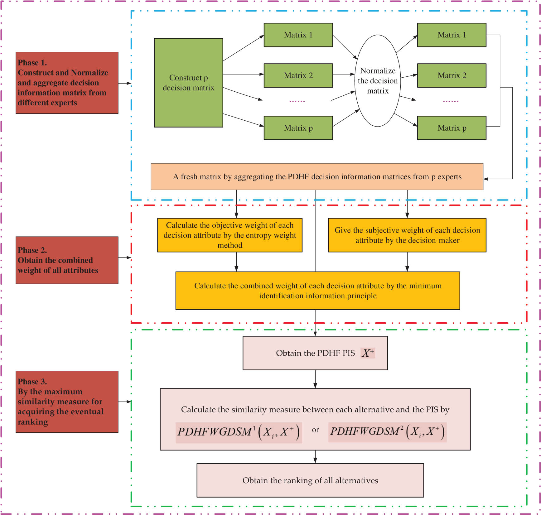
Flowchart of the built PDHF MAGDM method.
5 A case study and comparative analyses
5.1 Background
Since the end of the twentieth century, the development of China’s foreign trade has experienced from the 1.0 era of exhibition channel business development, the 2.0 era of Internet B2B (enterprise to enterprise) platform interaction, the 3.0 era of digital marketing channel, to today’s 4.0 era of Internet big data and cloud computing. At the same time, affected by the international financial crisis, the global supply chain tends to be flat and the world trade pattern is unpredictable. In this context, China’s traditional foreign trade model has been seriously challenged. If CBECs want to survive and develop, it is urgent to transform CBEC. However, despite the rapid development of China’s CBEC in recent years, the application level of China’s CBECs is still not high enough, or copy other successful enterprise cases, or blindly follow the trend, lacking certain scientificity. Therefore, the research of this article becomes very meaningful.
5.2 Decision process
We use the MAGDM method proposed in this article to demonstrate the effectiveness of the MAGDM method by using CBECP as an example for Company W in Guiyang City, Guizhou Province. Since Company W issued a bidding announcement requiring the CBECP, four companies with CBECP from Beijing, Wuhan, Chengdu, and Shenzhen have participated in the bidding. In order to evaluate the four companies more scientifically and reasonably, Company W selected three experts in the industry to rate the four companies from five aspects: system functions, service quality, platform, information quality, and cost. The data are in the form of PDHFEs, and four evaluation indexes are explained as follows:
System functions. The system function is to measure the characteristics required by the e-commerce system, such as ease of learning, safety and reliability, data analysis function, whether the system supports ERP, and flexibility is the system function quality that users pay more attention to. System function is an important function of e-commerce system.
Service quality. Platform service is the basis for the successful exchange of products and funds between buyers and sellers, and the most important function of CBECP. It determines whether business flow, capital flow, information flow, and logistics can flow smoothly between buyers and sellers; the service quality of the platform plays a critical role in elevating consumers to use the platform again. The integrity, convenience, reliability, security of platform services and consumers’ own shopping experience will indirectly affect the order conversion rate by affecting consumers’ satisfaction. This is also a key factor for enterprises to consider when choosing a platform.
Platform and information quality. Platform quality is the positioning characteristic of the platform. Whether the visits of the platform, the customer groups, and market distribution of the platform match the enterprise’s target market, as well as the main hot selling product types, platform marketing methods and platform operation management methods of the platform, can promote the successful promotion and trading of enterprise products. Information quality is the content of e-commerce. Intelligibility, accuracy, completeness, and timeliness are the determinants of high-quality information. If the buyer and the seller conduct transactions through the e-commerce platform, the platform must effectively transmit the latest and comprehensive product information and industry information between the supplier and the demander, so as to achieve the purpose of smooth information flow between the supplier and the demander, so as to realize the platform transaction, which is the basis of the characteristics of the platform.
Operating cost. The platform cost is based on the purpose of the buyer and the seller to realize the transaction with the platform as the medium, and the platform collects a certain proportion of operation and management expenses from both parties or one of them, such as platform entry fee, transaction commission, transaction handling fee, and marketing promotion fee. The charging items of different platforms are also different. Platform charging is not only related to the early investment of the enterprise’s operating cost, but also one of the important benchmarks to measure the enterprise’s final profit.
There are four CBECPs
PDHF decision information matrix given by
| Alternatives |
|
|
|
|
|---|---|---|---|---|
|
|
|
|
|
|
|
|
|
|
|
|
|
|
|
|
|
|
|
|
|
|
|
|
PDHF decision information matrix given by
| Alternatives |
|
|
|
|
|---|---|---|---|---|
|
|
|
|
|
|
|
|
|
|
|
|
|
|
|
|
|
|
|
|
|
|
|
|
PDHF decision information matrix given by
| Alternatives |
|
|
|
|
|---|---|---|---|---|
|
|
|
|
|
|
|
|
|
|
|
|
|
|
|
|
|
|
|
|
|
|
|
|
Next, we shall give some detailed steps to show the process of PDHF MAGDM technique that is used to select the best CBECP for Company W.
Step 1: Normalize information matrices. Among the four decision attributes given in this study,
Normalized PDHF decision information matrix given by
| Alternatives |
|
|
|
|
|---|---|---|---|---|
|
|
|
|
|
|
|
|
|
|
|
|
|
|
|
|
|
|
|
|
|
|
|
|
The normalized PDHF decision information matrix given by
| Alternatives |
|
|
|
|
|---|---|---|---|---|
|
|
|
|
|
|
|
|
|
|
|
|
|
|
|
|
|
|
|
|
|
|
|
|
Normalized PDHF decision information matrix given by
| Alternatives |
|
|
|
|
|---|---|---|---|---|
|
|
|
|
|
|
|
|
|
|
|
|
|
|
|
|
|
|
|
|
|
|
|
|
Step 2: Aggregate the PDHF decision information matrices from three experts to build a fresh decision information matrix by equation (40). The aggregated PDHF decision information matrix
Aggregated PDHF decision information matrix
| Alternatives |
|
|
|---|---|---|
|
|
|
|
|
|
|
|
|
|
|
|
|
|
|
|
| Alternatives |
|
|
|---|---|---|
|
|
|
|
|
|
|
|
|
|
|
|
|
|
|
|
Step 3: Calculate
Calculate
The calculation results are recorded in Table 9.
The information energy matrix
| Alternatives |
|
|
|
|
|---|---|---|---|---|
|
|
0.4546 | 0.2631 | 0.3419 | 0.4664 |
|
|
0.2127 | 0.2480 | 0.5363 | 0.1203 |
|
|
0.3340 | 0.2382 | 0.3666 | 0.2438 |
|
|
0.1973 | 0.1764 | 0.2900 | 0.1250 |
Combined weight
| Attribute |
|
|
|
|
|---|---|---|---|---|
| Entropy weight
|
0.2503 | 0.28 | 0.1973 | 0.2725 |
| Subjective weight
|
0.1 | 0.3 | 0.4 | 0.2 |
| Combined weight
|
0.1644 | 0.3011 | 0.2919 | 0.2426 |
Step 4: Determine the fuzzy PIS by equations (46) and (47), which are recorded in Table 10.
The PDHF PIS
| Attributes |
|
|
|---|---|---|
|
|
|
|
| Attributes |
|
|
|---|---|---|
|
|
|
|
Step 5: Calculate the similarity measure (SM) between each alternative and the PIS by equations (48) and (49), which are shown in Table 11.
The similarity measures with
| Alternatives |
|
|
|
|
ranking |
|---|---|---|---|---|---|
|
|
0.9727 | 0.8360 | 0.9277 | 0.7642 |
|
|
|
0.9616 | 0.8936 | 0.9195 | 0.7628 |
|
Step 6: Obtain the ranking of all alternatives by
Changes of four similarity degrees with parameter
Ranking of the four CBECPs with different
|
|
|
|
|
|
Ranking |
|---|---|---|---|---|---|
| 0 | 0.9089 | 0.6459 | 0.6913 | 0.4620 |
|
| 0.1 | 0.9191 | 0.6641 | 0.7247 | 0.4975 |
|
| 0.2 | 0.9305 | 0.6856 | 0.7625 | 0.5393 |
|
| 0.3 | 0.9436 | 0.7115 | 0.8055 | 0.5891 |
|
| 0.4 | 0.9588 | 0.7439 | 0.8551 | 0.6500 |
|
| 0.5 | 0.9765 | 0.7855 | 0.9132 | 0.7262 |
|
| 0.6 | 0.9975 | 0.8419 | 0.9824 | 0.8253 |
|
| 0.7 | 1.0228 | 0.9235 | 1.0670 | 0.9609 |
|
| 0.8 | 1.0538 | 1.0552 | 1.1737 | 1.1631 |
|
| 0.9 | 1.0926 | 1.3148 | 1.3143 | 1.5170 |
|
| 1 | 1.1428 | 2.1821 | 1.5122 | 2.4777 |
|
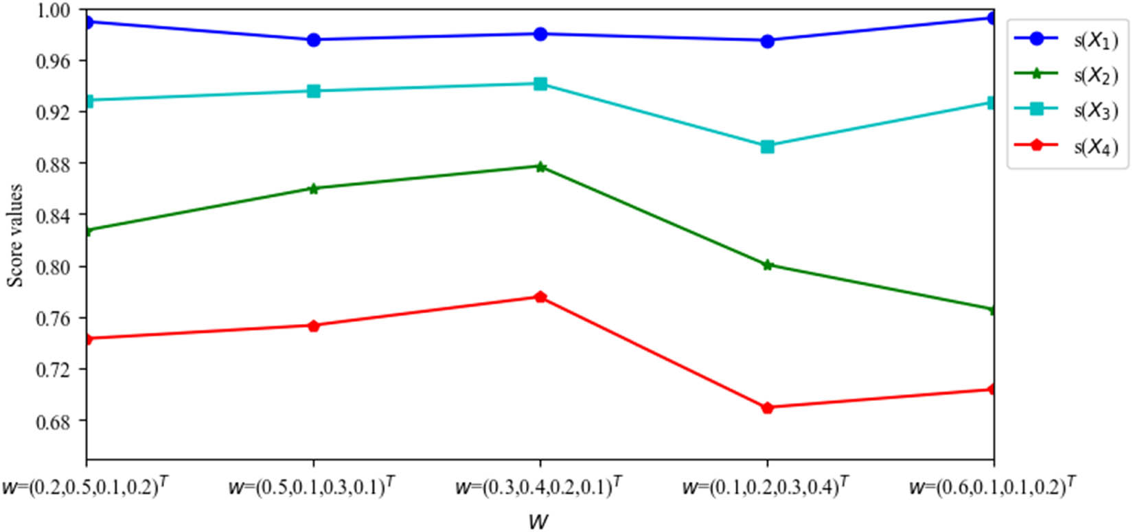
5.3 Sensitivity analysis of parameters
This study proposes an MAGDM technique in PDHF environment based on the newly proposed PDHFWGDSMs. It is obvious that the ranking of four CBECPs will be affected by the changes of several parameters:
The sequencing of the four CBECPs will be affected by the parameter
The ranking of the four CBECPs will be affected by
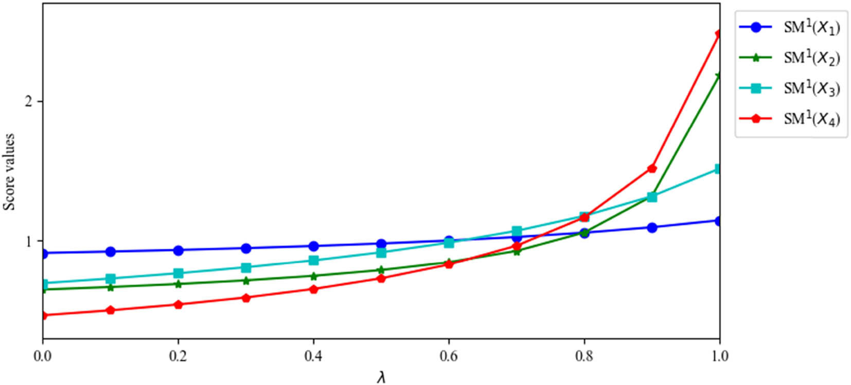
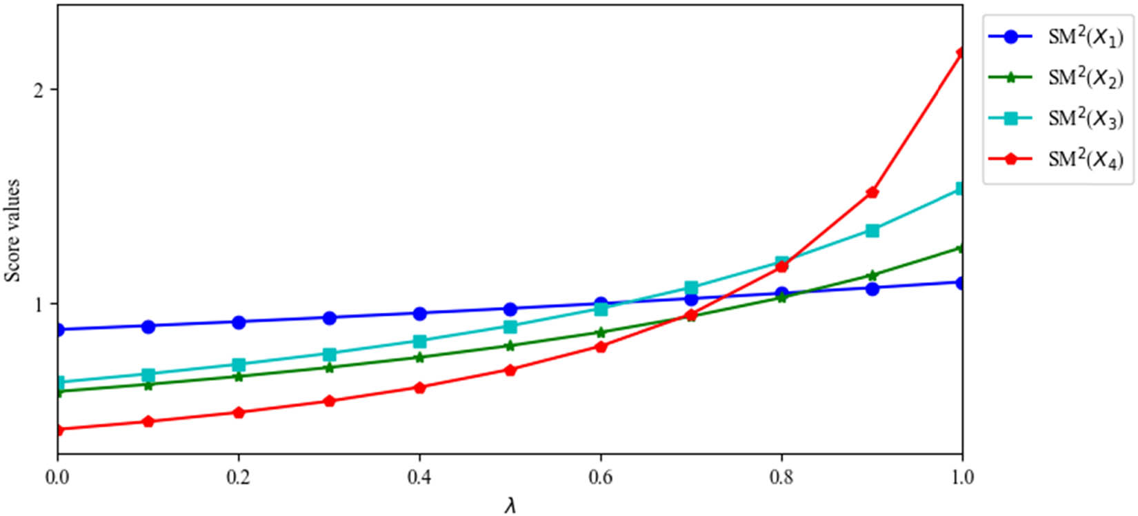
5.3.1 The sequencing of the four CBECPs changes with the change of parameter
λ
When
When
When
We can obtain from Table 13 and Figure 3 that when
Ranking of the four CBECPs with different
|
|
|
|
|
|
Ranking |
|---|---|---|---|---|---|
| 0 | 0.8761 | 0.5867 | 0.6295 | 0.4099 |
|
| 0.1 | 0.8942 | 0.6199 | 0.6690 | 0.4461 |
|
| 0.2 | 0.9131 | 0.6570 | 0.7138 | 0.4892 |
|
| 0.3 | 0.9329 | 0.6988 | 0.7650 | 0.5417 |
|
| 0.4 | 0.9535 | 0.7463 | 0.8241 | 0.6068 |
|
| 0.5 | 0.9750 | 0.8007 | 0.8931 | 0.6896 |
|
| 0.6 | 0.9975 | 0.8637 | 0.9747 | 0.7985 |
|
| 0.7 | 1.0211 | 0.9375 | 1.0727 | 0.9485 |
|
| 0.8 | 1.0459 | 1.0251 | 1.1926 | 1.1676 |
|
| 0.9 | 1.0718 | 1.1306 | 1.3428 | 1.5186 |
|
| 1 | 1.0991 | 1.2605 | 1.5361 | 2.1711 |
|
Changes of four similarity degrees with parameter
Ranking of the four CBECPs with different
|
|
|
|
|
|
Ranking |
|---|---|---|---|---|---|
|
|
0.9865 | 0.8218 | 0.9347 | 0.7654 |
|
|
|
0.9756 | 0.8196 | 0.9321 | 0.7524 |
|
|
|
0.9809 | 0.8463 | 0.9411 | 0.7801 |
|
|
|
0.9765 | 0.7855 | 0.9132 | 0.7262 |
|
|
|
0.9859 | 0.773 | 0.9248 | 0.7237 |
|
Ranking of the four CBECPs with different
|
|
|
|
|
|
Ranking |
|---|---|---|---|---|---|
|
|
0.9896 | 0.82714 | 0.92834 | 0.7431 |
|
|
|
0.9755 | 0.85980 | 0.93554 | 0.7534 |
|
|
|
0.98 | 0.87721 | 0.94136 | 0.7755 |
|
|
|
0.975 | 0.80074 | 0.89308 | 0.6896 |
|
|
|
0.9924 | 0.76601 | 0.92682 | 0.7036 |
|
Changes of four similarity degrees with weights
Changes of four similarity degrees with weights
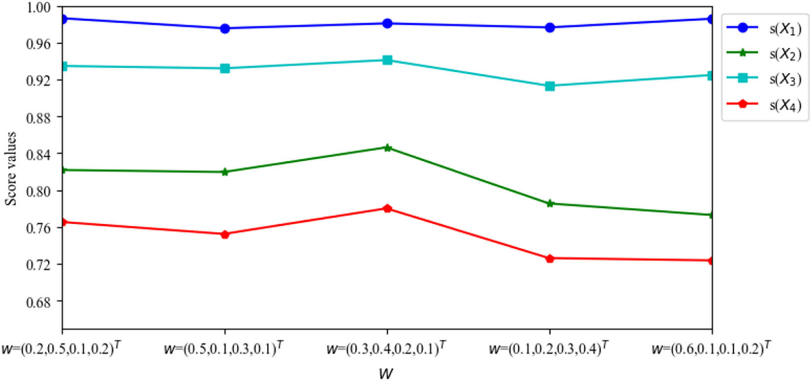
5.3.2 The sequencing of the four CBECPs changes with the change of parameter
w
We can see from Table 15 and Figure 5 that when
5.4 Validity analysis of the proposed MAGDM technique
In such section, we shall compare the MAGDM technique with several decision-making methods to investigate the validity of the proposed MAGDM technique. And the results are shown in Tables 16–19.
Outcome of four CBECPs
| Alternatives | PDHFWEA operator | Score values | The ranking |
|---|---|---|---|
|
|
|
0.2533 |
|
|
|
|
0.1415 | |
|
|
|
0.0114 | |
|
|
|
0.0368 |
Outcome of four CBECPs
| Alternatives | PDHFWEG operator | Score values | The ranking |
|---|---|---|---|
|
|
|
0.2363 |
|
|
|
|
−0.2414 | |
|
|
|
−0.068 | |
|
|
|
−0.0543 |
The outcome of four CBECPs
| Alternatives | PDHFWA operator | Score values | The ranking |
|---|---|---|---|
|
|
|
0.2566 |
|
|
|
|
−0.1261 | |
|
|
|
0.0005 | |
|
|
|
−0.0337 |
Outcome of four CBECPs
| Alternatives | PDHFWG operator | Score values | The ranking |
|---|---|---|---|
|
|
|
0.1006 |
|
|
|
|
−0.3937 | |
|
|
|
−0.1083 | |
|
|
|
−0.2294 |
5.4.1 Comparison with decision-making model of Garg and Kaur [42]
The data in Table 7 are substituted into equations (50) and (51), and
5.4.2 Comparison with decision-making model in the study
The data in Table 7 are substituted into PDHFWA and PDHFWG operators, and
5.4.3 Comparison with decision-making model of Ren et al. [41]
Step 1. Calculate the relative weight.
Step
2. Calculate the dominance of alternative
where
where
Step
3. Calculate the prospect value of
Step
4. The ranking can be obtained by
We substitute
Outcome of four CBECPs
| Alternatives |
|
|
The ranking |
|---|---|---|---|
|
|
−0.5651 | 1 |
|
|
|
−6.332 | 0.6918 | |
|
|
−8.1487 | 0.5941 | |
|
|
−19.247 | 0 |
5.4.4 Comparison with decision-making model of Ren et al. [65]
Step
1: Calculate
where
Step
2: Determine
where
Values of
| Alternatives |
|
|
|
The ranking |
|---|---|---|---|---|
|
|
0.0900 | 0.0900 | 0.0000 |
|
|
|
0.5959 | 0.2919 | 0.8584 | |
|
|
0.6652 | 0.2583 | 0.8308 | |
|
|
0.7552 | 0.3011 | 1.0000 |
Step
3. Finally, we can obtain the ranking according to
The data in Table 7 and
We can obtain the ranking, which is
5.5 Comprehensive analysis
According to the aforementioned comparative analysis and the research results of this study (Table 22 and Figure 6), we can obtain the best CBECP, which is always
Ranking of four CBECPs by using different methods
| Decision-making methods | The ranking |
|---|---|
| PDHFWEA operator |
|
| PDHFWEG operator |
|
| PDHFWA operator |
|
| PDHFWG operator |
|
| Traditional PDHF TODIM method |
|
| PDHF VIKOR method |
|
| Our proposed MAGDM technique by
|
|
| Our proposed MAGDM technique by
|
|
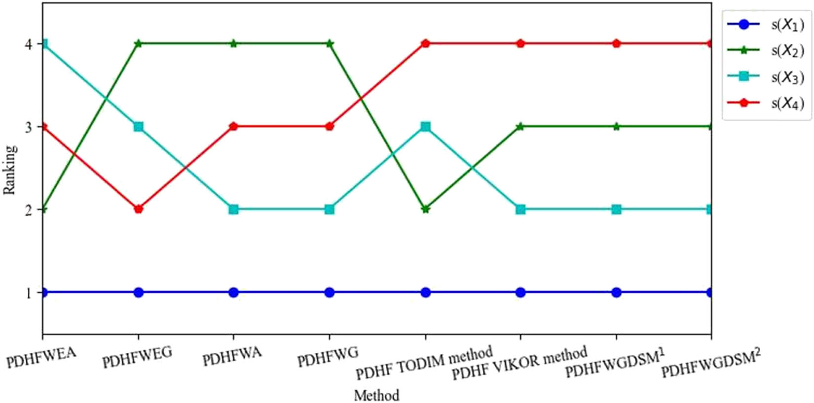
The ranking obtained by different decision-making methods.
6 Conclusions
Reasonable CBECPS is very important for the sustainable development of CBECs, and the design of scientific and reasonable CBECPS decision-making technique is the premise. This study designs an MAGDM technique for CBECPS. The contributions and limitations of MAGDM technique proposed in this study are as follows. The MAGDM problem is facing more and more complex situations. In some unpredictable emergencies or changing social environment, there are many incomplete, fuzzy, and inconsistent information. The MAGDM methods based on PDHFWGDSMs in the PDHF environment can provide DMs with suggestions for making the most appropriate choice in the complex reality environment. Specifically, this study made the following main contributions to solve the limitations of the existing literature and overcome the challenges of research gaps: (1) this study constructs a scientific and reasonable evaluation index system for CBECPS of CBEC, which is a crucial prerequisite; (2) we propose a new PDHF entropy without auxiliary functions to scientifically and reasonably weight for decision attributes; (3) a novel aggregation operator named as PDHFWG operator is proposed and used in the aggregation of PDHF information; (4) since DSM has been extended to many fuzzy environments, the DSM is extended to PDHF environment and six forms of DSM in PDHF environment are proposed, providing a new method for measuring the similarity between two PDHFSs; (5) this study applies the newly developed MAGDM methods to the CBECPS. Through comparative analysis and parameter analysis, it proves the applicability of the new technique and its advantages over the existing methods; (6) the newly proposed PDHF entropy, aggregation operator, and PDHFWGDSM of PDHFEs can provide some theoretical supplements to the in-depth study of PDHFS to a certain extent, and will play a very fundamental role in the rapid development of PDHFS.
However, this study may have some limitations: first, the MAGDM technique cannot solve the MAGDM problems in the IVIFS, q-ROF, q-RPDHF, and IVPDHF environments. Second, in this study, we only considered the combined weighting method of entropy weighting method and subjective weighting method, but did not consider the application of CRITIC method [66] and FUCOM method in decision-making methods. Therefore, the scientific and reasonable weighting method is also the prerequisite for scientific application of this method.
In the future research, we will focus on the research of new decision methods that combine PDHFS and current classic decision methods under the PDHF environment, continue to focus on the research of aggregation operators, and propose some new MAGDM methods. It is also committed to applying the decision-making methods proposed in this study to uncertain MAGDM problems, such as strategy selection, site selection, green supplier selection, clean energy selection, and optimal selection of talents,.
Acknowledgments
This work was supported by the The Scientific Research and Cultivation Project of Liupanshui Normal University (LPSSY2023KJZDPY08), Discipline Cultivation Team of Liupanshui Normal University(LPSSY2023XKPYTD04), Young Scientific and Technological Talents Growth Project of Guizhou Provincial Department of Education (Qian jiao he KY [2018]369, Qian jiao he KY [2018]385, and Qian jiao he KY [2017]274), and Science and Technology Innovation Team of Liupanshui Normal University (LPSSYKJTD201702). There is no individual participant included in the study.
-
Funding information: This work was supported by the Young Scientific and Technological Talents Growth Project of Guizhou Provincial Department of Education (Qian jiao he KY [2018]369, Qian jiao he KY [2018]385, and Qian jiao he KY [2017]274), and Science and Technology Innovation Team of Liupanshui Normal University (LPSSYKJTD201702). There is no individual participant included in the study.
-
Author contributions: All authors have accepted responsibility for the entire content of this manuscript and approved its submission.
-
Conflict of interest: The authors state no conflict of interest.
-
Ethical approval: The conducted research is not related to either human or animal use.
-
Data availability statement: All data generated or analyzed during this study are included in this published article.
References
[1] X. H. Zhang, D. P. Xu, and L. Xiao, Intelligent perception system of big data decision in cross-border e-commerce based on data fusion, J. Sens. 2021 (2021), 7021151.10.1155/2021/7021151Search in Google Scholar
[2] X. H. Zhang, Y. H. Cai, and L. Xiao, Visitor information system of cross-border E-commerce platform based on mobile edge computing, Mob. Inf. Syst. 2021 (2021), 1687820.10.1155/2021/1687820Search in Google Scholar
[3] D. L. Wang and W. W. Li, Optimization algorithm and simulation of supply chain coordination based on cross-border E-commerce network platform, Eurasip J. Wirel. Commun. Netw. 2021 (2021), 23.10.1186/s13638-021-01908-4Search in Google Scholar
[4] P. P. Sun and L. G. Gu, Optimization of cross-border E-commerce logistics supervision system based on internet of things technology, Complexity 2021 (2021), 4582838.10.1155/2021/4582838Search in Google Scholar
[5] C. Rui, Research on classification of cross-border E-commerce products based on image recognition and deep learning, IEEE Access 9 (2021), 108083–108090.10.1109/ACCESS.2020.3020737Search in Google Scholar
[6] C. W. Lu, G. H. Lin, T. J. Wu, I. H. Hu, and Y. C. Chang, Influencing factors of cross-border E-commerce consumer purchase intention based on wireless network and machine learning, Security Commun. Netw. 2021 (2021), 9984213.10.1155/2021/9984213Search in Google Scholar
[7] B. Li, J. H. Li, and X. J. Ou, Hybrid recommendation algorithm of cross-border e-commerce items based on artificial intelligence and multiview collaborative fusion, Neural Comput. Appl. (2021), DOI: https://doi.org/10.1007/s00521-00021-06249-00523.10.1007/s00521-021-06249-3Search in Google Scholar
[8] X. H. Chen, Semantic matching efficiency of supply and demand text on cross-border E-commerce online technology trading platforms, Wirel. Commun. Mob. Comput. 2021 (2021), 1–12, DOI: https://doi.org/10.1155/2021/9976774.10.1155/2021/9976774Search in Google Scholar
[9] S. Q. Li, Structure optimization of E-commerce platform based on artificial intelligence and blockchain technology, Wirel. Commun. Mob. Comput. 2020 (2020), 8825825.10.1155/2020/8825825Search in Google Scholar
[10] Y. Ma, A. Ruangkanjanases, and S. C. Chen, Investigating the impact of critical factors on continuance intention towards cross-border shopping websites, Sustainability 11 (2019), 5914.10.3390/su11215914Search in Google Scholar
[11] L. A. Zadeh, Fuzzy sets, Inf. Control 8 (1965), 338–353.10.1016/S0019-9958(65)90241-XSearch in Google Scholar
[12] A. Ashraf, K. Ullah, A. Hussain, and M. Bari, Interval-valued picture fuzzy Maclaurin symmetric mean operator with application in multiple attribute decision-making, Rep. Mech. Eng. 3 (2022), 210–226.10.31181/rme20020042022aSearch in Google Scholar
[13] M. Riaz and H. M. A. Farid, Picture fuzzy aggregation approach with application to third-party logistic provider selection process, Rep. Mech. Eng. 3 (2022), 227–236.10.31181/rme20023062022rSearch in Google Scholar
[14] M. Eminli and N. Guler, An improved Takagi-Sugeno fuzzy model with multidimensional fuzzy sets, J. Intell. Fuzzy Syst. 21 (2010), 277–287.10.3233/IFS-2010-0461Search in Google Scholar
[15] P. Husek, Modelling ellipsoidal uncertainty by multidimensional fuzzy sets, Expert. Syst. Appl. 39 (2012), 6967–6971.10.1016/j.eswa.2012.01.021Search in Google Scholar
[16] P. Manuel Martinez-Jimenez, J. Chamorro-Martinez, and J. M. Keller, Adaptive multidimensional fuzzy sets for texture modeling, Int. J. Approximate Reasoning 103 (2018), 288–302.10.1016/j.ijar.2018.10.006Search in Google Scholar
[17] A. Lima, E. S. Palmeira, B. Bedregal, and H. Bustince, Multidimensional fuzzy sets, IEEE Trans. Fuzzy Syst. 29 (2021), 2195–2208.10.1109/TFUZZ.2020.2994997Search in Google Scholar
[18] K. T. Atanassov, Intuitionistic fuzzy sets, Fuzzy Sets Syst. 20 (1986), 87–96.10.1016/S0165-0114(86)80034-3Search in Google Scholar
[19] A. N. Al-Kenani, R. Anjum, and S. Islam, Intuitionistic fuzzy prioritized aggregation operators based on priority degrees with application to multicriteria decision-making, J. Funct. Spaces 2022 (2022), 1–16.10.1155/2022/4751835Search in Google Scholar
[20] K. Pandey, A. Mishra, P. Rani, J. Ali, and R. Chakrabortty, Selecting features by utilizing intuitionistic fuzzy Entropy method, Decis. Making: Appl. Manag. Eng. 6 (2023), DOI: https://doi.org/10.31181/dmame07012023p.Search in Google Scholar
[21] Z. Chen and P. Liu, Intuitionistic fuzzy value similarity measures for intuitionistic fuzzy sets, Comput. Appl. Math. 41 (2022), 45.10.1007/s40314-021-01737-7Search in Google Scholar
[22] F. Ecer, An extended MAIRCA method using intuitionistic fuzzy sets for coronavirus vaccine selection in the age of COVID-19, Neural Comput. Appl. 34 (2022), 5603–5623.10.1007/s00521-021-06728-7Search in Google Scholar PubMed PubMed Central
[23] R. Gupta and S. Kumar, Intuitionistic fuzzy similarity-based information measure in the application of pattern recognition and clustering, Int. J. Fuzzy Syst. (2022).10.1007/s40815-022-01272-5Search in Google Scholar
[24] K. Atanassov and G. Gargov, Interval valued intuitionistic fuzzy sets, Fuzzy Sets Syst. 31 (1989), 343–349.10.1016/0165-0114(89)90205-4Search in Google Scholar
[25] Z. Wang, F. Xiao, and W. Ding, Interval-valued intuitionistic fuzzy Jenson-Shannon divergence and its application in multi-attribute decision making, Appl. Intell. 52 (2022), 16168–16184.10.1007/s10489-022-03347-0Search in Google Scholar
[26] C. Wang and J. Li, Project investment decision based on VIKOR interval intuitionistic fuzzy set, J. Intell. Fuzzy Syst. 42 (2022), 623–631.10.3233/JIFS-189735Search in Google Scholar
[27] S. Salimian, S. M. Mousavi, and J. Antucheviciene, An interval-valued intuitionistic fuzzy model based on extended VIKOR and MARCOS for sustainable supplier selection in organ transplantation networks for healthcare devices, Sustainability 14 (2022), 3795.10.3390/su14073795Search in Google Scholar
[28] A. Ohlan, Novel entropy and distance measures for interval-valued intuitionistic fuzzy sets with application in multi-criteria group decision-making, Int. J. Gen. Syst. 51 (2022), 1–28.10.1080/03081079.2022.2036138Search in Google Scholar
[29] V. Torra, Hesitant fuzzy sets, Int. J. Intell. Syst. 25 (2010), 529–539.10.1002/int.20418Search in Google Scholar
[30] T. Senapati, G. Chen, R. Mesiar, R. R. Yager, and A. Saha, Novel Aczel-Alsina operations-based hesitant fuzzy aggregation operators and their applications in cyclone disaster assessment, Int. J. Gen. Syst. 51 (2022) no. 5, 511–546.10.1080/03081079.2022.2036140Search in Google Scholar
[31] Z. Li, Y. Dou, B. Xia, K. Yang, and M. Li, System portfolio selection based on GRA method under hesitant fuzzy environment, J. Syst. Eng. Electron. 33 (2022), 120–133.10.23919/JSEE.2022.000013Search in Google Scholar
[32] R. Krishankumar, D. Pamucar, F. Cavallaro, and K. S. Ravichandran, Clean energy selection for sustainable development by using entropy-based decision model with hesitant fuzzy information, Environ. Sci. Pollut. Res. 29 (2022), 42973–42990.10.1007/s11356-022-18673-6Search in Google Scholar PubMed
[33] B. Zhu, Z. Xu, and M. Xia, Dual hesitant fuzzy sets, J. Appl. Math. 2012 (2012), 2607–2645.10.1155/2012/879629Search in Google Scholar
[34] Y. Ni, H. Zhao, Z. Xu, and Z. Wang, Multiple attribute decision-making method based on projection model for dual hesitant fuzzy set, Fuzzy Optim. Decis. Mak. 21 (2022) 263–289.10.1007/s10700-021-09366-9Search in Google Scholar
[35] Y. Wei and Q. Wang, New distances for dual hesitant fuzzy sets and their application in clustering algorithm, J. Intell. Fuzzy Syst. 41 (2021), 6221–6232.10.3233/JIFS-202846Search in Google Scholar
[36] D. Tripathi, S. K. Nigam, A. R. Mishra, and A. R. Shah, A novel intuitionistic fuzzy distance measure-SWARA-COPRAS method for multi-criteria food waste treatment technology selection, Operational Res. Eng. Sci. Theory Appl. (2022), DOI: https://doi.org/10.31181/dmame07012023p.10.31181/dmame07012023pSearch in Google Scholar
[37] Z. Ali, T. Mahmood, K. Ullah, and Q. Khan, Einstein geometric aggregation operators using a novel complex interval-valued pythagorean fuzzy setting with application in green supplier chain management, Rep. Mech. Eng. 2 (2021), 105–134.10.31181/rme2001020105tSearch in Google Scholar
[38] B. Limboo and P. Dutta, A q-rung orthopair basic probability assignment and its application in medical diagnosis, Decis. Making: Appl. Manag. Eng. 5 (2022), 290–308.10.31181/dmame191221060lSearch in Google Scholar
[39] Z. N. Hao, Z. S. Xu, H. Zhao, and Z. Su, Probabilistic dual hesitant fuzzy set and its application in risk evaluation, Knowl. Syst. 127 (2017), 16–28.10.1016/j.knosys.2017.02.033Search in Google Scholar
[40] G. Anusha, P. V. Ramana, and R. Sarkar, Hybridizations of Archimedean copula and generalized MSM operators and their applications in interactive decision-making with q-rung probabilistic dual hesitant fuzzy environment, Decis. Making: Appl. Manag. Eng. (2022), DOI: https://doi.org/10.31181/dmame0329102022a.10.31181/dmame0329102022aSearch in Google Scholar
[41] Z. L. Ren, Z. S. Xu, and H. Wang, An extended TODIM method under probabilistic dual hesitant fuzzy information and its application on enterprise strategic assessment, 2017 IEEE International Conference on Industrial Engineering and Engineering Management (IEEM), (2017), pp. 1464–1468.10.1109/IEEM.2017.8290136Search in Google Scholar
[42] H. Garg and G. Kaur, Algorithm for probabilistic dual hesitant fuzzy multi-criteria decision-making based on aggregation operators with new distance measures, Mathematics 6 (2018), 280.10.3390/math6120280Search in Google Scholar
[43] H. Garg and G. Kaur, A robust correlation coefficient for probabilistic dual hesitant fuzzy sets and its applications, Neural Comput. Appl. 32 (2020), 8847–8866.10.1007/s00521-019-04362-ySearch in Google Scholar
[44] H. Garg and G. Kaur, Quantifying gesture information in brain hemorrhage patients using probabilistic dual hesitant fuzzy sets with unknown probability information, Comput. & Ind. Eng. 140 (2020), 106211.10.1016/j.cie.2019.106211Search in Google Scholar
[45] Q. Zhao, Y. B. Ju, and W. Pedrycz, A method based on bivariate almost stochastic dominance for multiple criteria group decision making with probabilistic dual hesitant fuzzy information, IEEE Access 8 (2020), 203769–203786.10.1109/ACCESS.2020.3035906Search in Google Scholar
[46] H. Garg and G. Kaur, Algorithms for screening travelers during COVID-19 outbreak using probabilistic dual hesitant values based on bipartite graph theory, Appl. Comput. Math. 20 (2021), 22–48.Search in Google Scholar
[47] X. Wang, H. Wang, Z. Xu, and Z. Ren, Green supplier selection based on probabilistic dual hesitant fuzzy sets: A process integrating best worst method and superiority and inferiority ranking, Appl. Intell. 52 (2021), 8279–8301.10.1007/s10489-021-02821-5Search in Google Scholar
[48] Z. Li, X. Zhang, W. Wang, and Z. Li, Multi-criteria probabilistic dual hesitant fuzzy group decision making for supply chain finance credit risk assessments, Expert. Syst. 39 (2022), no. 8, e13015.10.1111/exsy.13015Search in Google Scholar
[49] B. Ning, F. Lei, and G. Wei, CODAS method for multi-attribute decision-making based on some novel distance and entropy measures under probabilistic dual hesitant fuzzy sets, Int. J. Fuzzy Syst. 24 (2022), 3626–3649.10.1007/s40815-022-01350-8Search in Google Scholar
[50] B. Ning, G. Wei, and Y. Guo, Some novel distance and similarity measures for probabilistic dual hesitant fuzzy sets and their applications to MAGDM, Int. J. Mach. Learn. Cybern. 13 (2022), 3887–3907.10.1007/s13042-022-01631-6Search in Google Scholar
[51] B. Ning, G. Wei, R. Lin, and Y. Guo, A novel MADM technique based on extended power generalized Maclaurin symmetric mean operators under probabilistic dual hesitant fuzzy setting and its application to sustainable suppliers selection, Expert. Syst. Appl. 204 (2022), 117419.10.1016/j.eswa.2022.117419Search in Google Scholar
[52] B. Ning, R. Lin, G. Wei, and X. Chen, EDAS method for multiple attribute group decision making with probabilistic dual hesitant fuzzy information and its application to suppliers selection, Technol. Economic Dev. Econ. 29 (2023), 326–352.10.3846/tede.2023.17589Search in Google Scholar
[53] L. Dice, Measures of the amount of ecologic association between species, Ecology 26 (1945), 297–302.10.2307/1932409Search in Google Scholar
[54] H. Garg, Z. Ali, and T. Mahmood, Generalized dice similarity measures for complex q-Rung Orthopair fuzzy sets and its application, Complex. Intell. Syst. 7 (2021), 667–686.10.1007/s40747-020-00203-xSearch in Google Scholar
[55] N. Jan, L. Zedam, T. Mahmood, E. Rak, and Z. Ali, Generalized dice similarity measures for q-rung orthopair fuzzy sets with applications, Complex. Intell. Syst. 6 (2020), 545–558.10.1007/s40747-020-00145-4Search in Google Scholar
[56] A. Singh and S. Kumar, A novel dice similarity measure for IFSs and its applications in pattern and face recognition, Expert. Syst. Appl. 149 (2020), 113245.10.1016/j.eswa.2020.113245Search in Google Scholar
[57] J. Wang, H. Gao, and G. W. Wei, The generalized Dice similarity measures for Pythagorean fuzzy multiple attribute group decision making, Int. J. Intell. Syst. 34 (2019), 1158–1183.10.1002/int.22090Search in Google Scholar
[58] G. W. Wei and H. Gao, The generalized dice similarity measures for picture fuzzy sets and their applications, Informatica 29 (2018), 107–124.10.15388/Informatica.2018.160Search in Google Scholar
[59] S. Q. Zhang, G. W. Wei, R. Wang, J. Wu, C. Wei, Y. F. Guo, et al., Improved CODAS method under picture 2-tuple linguistic environment and its application for a green supplier selection, Informatica. 32 (2021), 195–216.10.15388/20-INFOR414Search in Google Scholar
[60] F. Lei, G. W. Wei, and X. D. Chen, Model-based evaluation for online shopping platform with probabilistic double hierarchy linguistic CODAS method, Int. J. Intell. Syst. 36 (2021), 5339–5358.10.1002/int.22514Search in Google Scholar
[61] D. H. Zhang, X. M. You, S. Liu, and K. Yang, Multi-colony ant colony optimization based on generalized Jaccard similarity recommendation strategy, IEEE Access 7 (2019), 157303–157317.10.1109/ACCESS.2019.2949860Search in Google Scholar
[62] G. W. Wei, C. Wei, J. Wu, and Y. F. Guo, Probabilistic linguistic multiple attribute group decision making for location planning of electric vehicle charging stations based on the generalized Dice similarity measures, Artif. Intell. Rev. 54 (2021), 4137–4167.10.1007/s10462-020-09950-2Search in Google Scholar
[63] Z. S. Xu and W. Zhou, Consensus building with a group of decision makers under the hesitant probabilistic fuzzy environment, Fuzzy Optim. Decis. Mak. 16 (2017), 481–503.10.1007/s10700-016-9257-5Search in Google Scholar
[64] D. Dumitrescu, A definition of an informational energy in fuzzy sets theory, Studia Univ. Babe? -Bolyai Math. 22 (1977), 57–59.Search in Google Scholar
[65] Z. L. Ren, Z. S. Xu, and H. Wang, The strategy selection problem on artificial intelligence with an integrated VIKOR and AHP method under probabilistic dual hesitant fuzzy information, IEEE Access 7 (2019), 103979–103999.10.1109/ACCESS.2019.2931405Search in Google Scholar
[66] M. Žižović, B. Miljković, and D. Marinković, Objective methods for determining criteria weight coefficients: A modification of the CRITIC method, Decis. Making: Appl. Manag. Eng. 3 (2020), 149–161.10.31181/dmame2003149zSearch in Google Scholar
© 2023 the author(s), published by De Gruyter
This work is licensed under the Creative Commons Attribution 4.0 International License.
Articles in the same Issue
- Regular Articles
- A novel class of bipolar soft separation axioms concerning crisp points
- Duality for convolution on subclasses of analytic functions and weighted integral operators
- Existence of a solution to an infinite system of weighted fractional integral equations of a function with respect to another function via a measure of noncompactness
- On the existence of nonnegative radial solutions for Dirichlet exterior problems on the Heisenberg group
- Hyers-Ulam stability of isometries on bounded domains-II
- Asymptotic study of Leray solution of 3D-Navier-Stokes equations with exponential damping
- Semi-Hyers-Ulam-Rassias stability for an integro-differential equation of order 𝓃
- Jordan triple (α,β)-higher ∗-derivations on semiprime rings
- The asymptotic behaviors of solutions for higher-order (m1, m2)-coupled Kirchhoff models with nonlinear strong damping
- Approximation of the image of the Lp ball under Hilbert-Schmidt integral operator
- Best proximity points in ℱ-metric spaces with applications
- Approximation spaces inspired by subset rough neighborhoods with applications
- A numerical Haar wavelet-finite difference hybrid method and its convergence for nonlinear hyperbolic partial differential equation
- A novel conservative numerical approximation scheme for the Rosenau-Kawahara equation
- Fekete-Szegö functional for a class of non-Bazilevic functions related to quasi-subordination
-
On local fractional integral inequalities via generalized
- On some geometric results for generalized k-Bessel functions
- Convergence analysis of M-iteration for 𝒢-nonexpansive mappings with directed graphs applicable in image deblurring and signal recovering problems
- Some results of homogeneous expansions for a class of biholomorphic mappings defined on a Reinhardt domain in ℂn
- Graded weakly 1-absorbing primary ideals
- The existence and uniqueness of solutions to a functional equation arising in psychological learning theory
- Some aspects of the n-ary orthogonal and b(αn,βn)-best approximations of b(αn,βn)-hypermetric spaces over Banach algebras
- Numerical solution of a malignant invasion model using some finite difference methods
- Increasing property and logarithmic convexity of functions involving Dirichlet lambda function
- Feature fusion-based text information mining method for natural scenes
- Global optimum solutions for a system of (k, ψ)-Hilfer fractional differential equations: Best proximity point approach
- The study of solutions for several systems of PDDEs with two complex variables
- Regularity criteria via horizontal component of velocity for the Boussinesq equations in anisotropic Lorentz spaces
- Generalized Stević-Sharma operators from the minimal Möbius invariant space into Bloch-type spaces
- On initial value problem for elliptic equation on the plane under Caputo derivative
- A dimension expanded preconditioning technique for block two-by-two linear equations
- Asymptotic behavior of Fréchet functional equation and some characterizations of inner product spaces
- Small perturbations of critical nonlocal equations with variable exponents
- Dynamical property of hyperspace on uniform space
- Some notes on graded weakly 1-absorbing primary ideals
- On the problem of detecting source points acting on a fluid
- Integral transforms involving a generalized k-Bessel function
- Ruled real hypersurfaces in the complex hyperbolic quadric
- On the monotonic properties and oscillatory behavior of solutions of neutral differential equations
- Approximate multi-variable bi-Jensen-type mappings
- Mixed-type SP-iteration for asymptotically nonexpansive mappings in hyperbolic spaces
- On the equation fn + (f″)m ≡ 1
- Results on the modified degenerate Laplace-type integral associated with applications involving fractional kinetic equations
- Characterizations of entire solutions for the system of Fermat-type binomial and trinomial shift equations in ℂn#
- Commentary
- On I. Meghea and C. S. Stamin review article “Remarks on some variants of minimal point theorem and Ekeland variational principle with applications,” Demonstratio Mathematica 2022; 55: 354–379
- Special Issue on Fixed Point Theory and Applications to Various Differential/Integral Equations - Part II
- On Cauchy problem for pseudo-parabolic equation with Caputo-Fabrizio operator
- Fixed-point results for convex orbital operators
- Asymptotic stability of equilibria for difference equations via fixed points of enriched Prešić operators
- Asymptotic behavior of resolvents of equilibrium problems on complete geodesic spaces
- A system of additive functional equations in complex Banach algebras
- New inertial forward–backward algorithm for convex minimization with applications
- Uniqueness of solutions for a ψ-Hilfer fractional integral boundary value problem with the p-Laplacian operator
- Analysis of Cauchy problem with fractal-fractional differential operators
- Common best proximity points for a pair of mappings with certain dominating property
- Investigation of hybrid fractional q-integro-difference equations supplemented with nonlocal q-integral boundary conditions
- The structure of fuzzy fractals generated by an orbital fuzzy iterated function system
- On the structure of self-affine Jordan arcs in ℝ2
- Solvability for a system of Hadamard-type hybrid fractional differential inclusions
- Three solutions for discrete anisotropic Kirchhoff-type problems
- On split generalized equilibrium problem with multiple output sets and common fixed points problem
- Special Issue on Computational and Numerical Methods for Special Functions - Part II
- Sandwich-type results regarding Riemann-Liouville fractional integral of q-hypergeometric function
- Certain aspects of Nörlund ℐ-statistical convergence of sequences in neutrosophic normed spaces
- On completeness of weak eigenfunctions for multi-interval Sturm-Liouville equations with boundary-interface conditions
- Some identities on generalized harmonic numbers and generalized harmonic functions
- Study of degenerate derangement polynomials by λ-umbral calculus
- Normal ordering associated with λ-Stirling numbers in λ-shift algebra
- Analytical and numerical analysis of damped harmonic oscillator model with nonlocal operators
- Compositions of positive integers with 2s and 3s
- Kinematic-geometry of a line trajectory and the invariants of the axodes
- Hahn Laplace transform and its applications
- Discrete complementary exponential and sine integral functions
- Special Issue on Recent Methods in Approximation Theory - Part II
- On the order of approximation by modified summation-integral-type operators based on two parameters
- Bernstein-type operators on elliptic domain and their interpolation properties
- A class of strongly convergent subgradient extragradient methods for solving quasimonotone variational inequalities
- Special Issue on Recent Advances in Fractional Calculus and Nonlinear Fractional Evaluation Equations - Part II
- Application of fractional quantum calculus on coupled hybrid differential systems within the sequential Caputo fractional q-derivatives
- On some conformable boundary value problems in the setting of a new generalized conformable fractional derivative
- A certain class of fractional difference equations with damping: Oscillatory properties
- Weighted Hermite-Hadamard inequalities for r-times differentiable preinvex functions for k-fractional integrals
- Special Issue on Recent Advances for Computational and Mathematical Methods in Scientific Problems - Part II
- The behavior of hidden bifurcation in 2D scroll via saturated function series controlled by a coefficient harmonic linearization method
- Phase portraits of two classes of quadratic differential systems exhibiting as solutions two cubic algebraic curves
- Petri net analysis of a queueing inventory system with orbital search by the server
- Asymptotic stability of an epidemiological fractional reaction-diffusion model
- On the stability of a strongly stabilizing control for degenerate systems in Hilbert spaces
- Special Issue on Application of Fractional Calculus: Mathematical Modeling and Control - Part I
- New conticrete inequalities of the Hermite-Hadamard-Jensen-Mercer type in terms of generalized conformable fractional operators via majorization
- Pell-Lucas polynomials for numerical treatment of the nonlinear fractional-order Duffing equation
- Impacts of Brownian motion and fractional derivative on the solutions of the stochastic fractional Davey-Stewartson equations
- Some results on fractional Hahn difference boundary value problems
- Properties of a subclass of analytic functions defined by Riemann-Liouville fractional integral applied to convolution product of multiplier transformation and Ruscheweyh derivative
- Special Issue on Development of Fuzzy Sets and Their Extensions - Part I
- The cross-border e-commerce platform selection based on the probabilistic dual hesitant fuzzy generalized dice similarity measures
- Comparison of fuzzy and crisp decision matrices: An evaluation on PROBID and sPROBID multi-criteria decision-making methods
- Rejection and symmetric difference of bipolar picture fuzzy graph