Visual Analysis of Cylindrically Polarized Light Beams’ Focal Characteristics by Path Integral
-
Cheng-feng Yue


Abstract
To analyze the focal characteristics of cylindrically polarized beams, a visual analysis method is proposed. As known, the focal field can be described by three mutually perpendicular components, each one is the total contribution of all parts of the incident beams. For each component of all contributing parts weapply path integral method, then from the path integral curves extract focal field properties immediately, such as polarization state or intensity distribution. The analysis process of PI is visual and more understandable, and has more powerful information extraction function, which is also helpful for the design of special filtering pupil.
1 Introduction
Over the years, the special focal characteristics of cylindrically polarized (CP) beams have attracted much interest [1, 2, 3, 4, 5, 6, 7, 8, 9, 10, 11, 12, 13]. CP beams are also referred as radially polarized (RP) and azimuthally polarized (AP) beams. The special intensity distribution of CP beams on the focal plane has many wide applications. For example, the donut intensity distribution of AP beams can be used in particle trapping [14, 15, 16, 17]. The tight focal spot of the longitudinal field of RP beams is useful in improving the resolution of confocal microscopy [18, 19, 20, 21] and optical data storage [22, 23].
The basic theory by which focused polarized beams can be analyzed was originally described by Richards and Wolf [1, 2] in 1959 and remains the basic principle of vector beams’ focal problems until now. However, the role of every part that contributes to the focal field cannot be evaluated easily using only algebraic integral calculation, and the results are somewhat puzzling. To overcome these drawbacks, a visual analysis method was proposed that focuses on the path integral(PI) curves rather than purely on mathematical equations.
Contrary to algebraic integral, the advantage of PI is its intuition and understandability. The use of PI will be beneficial to the analysis of vector beams focusing problems, and the combination of PI and algebraic calculation can extract more information, more easily and comprehensively.
2 Theory of PI
Initially, the concept of PI was proposed in the 1940s by American physicist Feynman [24] for expressing quantum amplitude. Later Feynman used PI to illustrate the superposition of coherent light. For revealing the essence of Fermat’s principle, Feynman described the mirror reflection phenomenon by PI method. He divided the mirror into many small pieces as shown in Figure 1(a). According to the diffraction theory, every ray of light reflected from S point through the mirror to P point may hold, and their amplitudes are same, but the phases are different because of the different paths. So, Feynman represented them with arrows in different directions, as shown in Figure 1(b). The light field of point P denoted by vector
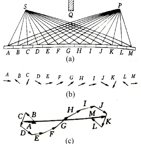
The illustration of Fermat’s Path Integral principle : the image of mirror reflection
3 Basic focal theory of CP beams
Figure 2 shows the geometry of the focal system.According to Richards and Wolf theory, the electric field at point Q generated by RP and AP beams near point P can be written

Focal system geometry.Σ1 is the equal phase spherical surface just after the lens.ΣF is the focal plane. O is the center of the lens. F is the focus. P and Q are points on Σ1 andΣF, respectively, and Φ and ΦQ are the azimuth angles of P and Q respectively. θ is the diffraction angle of light PF. Δθ is the angle width of the annular beams
as
where φ denotes the azimuth relative to the x-axis. θ is the semi-angular aperture of the annular beams. A0 (θ) is the light beams’ amplitude distribution, which is supposed
to be constant A0. ≥ and f are the wavelength and focal length. ρQ is the distance of point Q to focus F. φQ is the azimuth of Q to the x-axis.
A clear circular aperture can always be treated as the sum of many annular rings with different radius; thus, the focal properties of a narrow (with angular width Δθ << π/2) annular beams are studied here. In fact, using large numerical annular beams to achieve a tight focus has been proposed by many papers [25, 26, 27]. Here suppose the annular beams numerical aperture(N.A) is 1.
4 RP beams’ focal properties
4.1 Transverse focal properties
The annular beams shown in Figure 2 can be separated into a number of small facets (here supposed separated into M), each one with an angle width ΔθΔφ, where Δφ = 2π/M. Each facet contributes to the field on Q, so according equation (1), the field on Q is
where
m is a cosine function of mΔφ with amplitude k0ρ0N.A. When m changes from 0 to M, m gets all of its values in one cycle as shown in Figure 3.
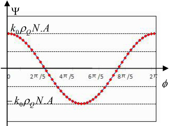
Phase values on point Q generated by all small fifty facets on the annular beams. Phi is the azimuth of the facets, and Φm = mΔφ
By applying PI to describe formulas (2) and (3), Figure 4 is achieved. In Figure 4, on the curves, between each two neighbor points there is a small vector and each vector denotes the contribution of one small facet to the field on point Q. The small vector’s length and direction represent its amplitude and phase respectively. ζ and η are the assistant phase reference axes, and ζ -axis denotes zero phase, and all other direction angles of the small vectors to ζ -axis denote their phase m. There, the first and the last vectors represent respectively the contribution of point P with φ = 0 and φM = (M − 1) * 2π/M. All M vectors link together, starting from A and ending at B, thus,

The PI curves of all small vectors generated by small facets on annular beams. The ζ axis indicates the direction of reference phase zero, and the η axis indicates π/2 relative phase. Here, all the values are relative to
Figure 4(a) shows PI curves on Q1 (ρQ = λ/8, φ0 = π/4), where

The transverse components PI curves generated by RP annular (N.A.=1) beams on 11 points with φQ = 0, ρQi = 2(i − 1)λ/50, j=1,2…11. All curves are normalized by the largest value
4.2 Longitudinal focal properties
According to formula (2), the longitudinal field of point Q generated by all facets on annular beams can be written as
where
Using PI to express formula(6), we got Figure 6. There are eleven curves corresponding to eleven points Qi with

The longtitudinal component PI curves generated by RP annular beams (N.A=1). Corresponding to ρQj = (2j − 1)λ/50 (j=1,2…11) φQ = 0 respectively, there are 11 curves. All curves are normalized by the largest value
plane locates at about
4.3 Polarization state on the RP focal plane
The polarization state of the total field is determined by the phase difference between the transverse and longitudinal fields. Firstly, Figure 5 indicates that there is no transverse field in the center, so the field on axis is linearly polarized along the z-axis. Secondly, for an off-axis point, the transverse vector is always along η, while the longitudinal vector is always along ζ , so there is always π/2 phase difference between them, so the field is elliptically polarized with z and r as the symmetry axis as shown in Figure 7, and the long and short axis of the ellipse are determined by the weights of the transverse and longitudinal components.

The polarization state distribution on the focal plane generated by RP annular beams. ΣZr is the plane defined by z and r. “→” denotes the polarization direction
5 AP beams focal properties
Produced by annular beams with N.A=1 at Q (ρQ = λ/8, φQ = 0) on the focal plane, the PI graphs of x and y polarized components are shown in Figure 8, where all values are relative to

The PI curves on Q (ρQ = λ/8, φQ = 0) produced by AP annular beams. Other parameters are the same as those in Figure 3. Here, the value is relative to˜C3(θ)
In fact, this relationship is coincident with Formula (1), only by considering cos θ is a constant weight.
Figure 8 indicates that
Formula (1), Figure 4(b) and Figure 8 indicate that the focal field intensity of the AP beams is similar to the transverse component of RP beams’, written as
There for, the transverse component of RP beams’ is donut on focal plane, so AP beam’s focal field is donut too.
6 Conclusion
Figure 9 shows the transverse, longitudinal and total intensity distribution on focal plane generated by RP annular beams with N.A=1(aperture angle θ = 0.23π, index n = 1.5), which is calculated by formula (1) using algebraic integral. It can be seen that the intensity distribution’s characteristics obtained by PI, such as the field construction and the location of extreme points, are consistent with those obtained by pure algebraic integral, which shows the effectiveness of the PI method in analyzing the focusing of vector beams.

The transverse (IT), longitudinal (IL) and total (Itotal) intensity distribution on focal plane generated by RP annular beams with N.A=1 (aperture angle θ = 0.23π, index n = 1.5). Calculated by algebraic integral
But, in Figure 9, we only can see intensity distribution on focal plane, we can’t see more detailed information, nor can we see the specific effect of each incident ray on the final results either. In contrast, PI has obvious advantages. More information of focal field can be extracted directly from PI curves. For example, from Figure 4, we can get the polarization state of the transverse field at the focal plane. While comparing Figure 4 and Figure 5, the phase difference between the transverse field and the longitudinal field can be obtained directly, then the total polarization state on the focal plane can be calculated. According to Figure 5, the RP beams’ transverse field’s doughnut structure can be predicted. By the changing trend of the PI curves in Figure 6, the position of the ‘0’ field can be found. Figure 4(b) together with Figure 8 directly reveal the relationship between AP beams and transverse component of RP beams on focal plane. All above examples indicate that PI has more powerful information extraction function. Those obvious information in PI curves is easily submerged in the pure algebra integral calculating.
At the same time, PI also intuitively illustrate the effect of each part of the incident beam on the results, so when special focus field is needed, such as a tighter focusing, the use of PI will greatly improve the initiative in the designing of filter pupil.
Take the advantage of PI, even the focus field polarization distribution can be modulated, For example, according to Figure 4(b) and Figure 6, if half-wavelength filter is used in the half-space bounded by x-axis, it is easy to conclude that the x and longitudinal components will be zero, while the original zero y-polarization component will no longer be zero, that means the field on the x-axis will change from elliptical polarized to y-direction linear polarized light. So with the help of PI analysis, it’s hopeful to design appropriate filter pupil to modulate light beams to meet different polarization requirements, which will be of great use in atomic capturing and manipulating, optical information coding, etc.
Acknowledgement
This work was supported by National Natural Science Foundation of China (Grant No. 61575067)
References
[1] Richards B., Wolf E. , Electromagnetic diffraction in optical systems II. Structure of the image field in an aplanatic system., Proc. Roy. Soc. A 1959, 253, 358-379.10.1098/rspa.1959.0200Suche in Google Scholar
[2] Youngworth K.S., Brown T. G., Focusing of high numerical aperture cylindrical-vector beams., Opt. Express, 2000, 7(2), 78-87.10.1364/OE.7.000077Suche in Google Scholar
[3] Quabis S., Dorn R., Eberler M., GlÖckl O., Leuchs G. , Focusing light to a tighter spot., Opt. Commun. 2000, 179, 1-7.10.1016/S0030-4018(99)00729-4Suche in Google Scholar
[4] Erdélyi M., Bor Zs., Radial and azimuthal polarizers., J.Opt.A, Pure Appl.Opt, 2006, 8, 737-742.10.1088/1464-4258/8/9/005Suche in Google Scholar
[5] Gilad M.L., Uriel L., Effect of radial polarization and apodization on spot size under tight focusing conditions., Opt. Express, 2008, 16(7),4567-4581.10.1364/OE.16.004567Suche in Google Scholar PubMed
[6] Suresh P., Mariyal C., Gokulakrishnan K., Rajesh K. B., Pillai T. V. S., Jaroszewicz Z., Investigation the focus shaping of the TEM11* beam with radial varying polarization., Optik, 2015, 126, 1691-1694.10.1016/j.ijleo.2015.05.001Suche in Google Scholar
[7] Li J., Feng K., Guo L., Phase filter design for sharper focus of radially polarized beam., Optik, 2014, 125, 3690-3692.10.1016/j.ijleo.2014.01.132Suche in Google Scholar
[8] Wang Y., Qiu L., Zhao W., High precision radially-polarized -light pupil-filtering differential confocal measurement., Opt. Laser Technol., 2016, 82, 87-93.10.1016/j.optlastec.2016.02.005Suche in Google Scholar
[9] Dorn R., Quabis S., Leuch G., Sharper Focus for a Radially Polarized Light Beam., Phs.Rev.Lett., 2003, 91(23), 233901, 1-4.10.1103/PhysRevLett.91.233901Suche in Google Scholar PubMed
[10] Grosjean T., Suarez M., Sabac A., Generation of polychromatic radially and azimuthally polarized beams., Appl. Phys.Lett., 2008, 93, 231106.10.1063/1.3040056Suche in Google Scholar
[11] Hua Y., Wang Z., Li H., Nan G., Du Y., Radially and Azimuthally Polarized Beams Generated by a Composite Spiral Zone Plate., ChIN. PHYS. LETT., 2012, 29(8), 08214.10.1088/0256-307X/29/8/084214Suche in Google Scholar
[12] Wang F., Zhao C., Dong Y., Generation and tight-focusing properties of cylindrical vector circular Airy beams., Appl.Phys.B., 2014, 117, 905-913.10.1007/s00340-014-5908-9Suche in Google Scholar
[13] Wang X., Ren H., Nah Ch., Linearly to radially polarized light conversion and tight focus., J. Appl. Phys., 2015, 117, 243101.10.1063/1.4923050Suche in Google Scholar
[14] Kotlyar V. V., Nalimov A. G., Analytical expression for radiation forces on a dielectric cylinder illuminated by a cylindrical Gaussian beam., Opt. Express, 2006, 14, 6136–6321.10.1364/OE.14.006316Suche in Google Scholar
[15] Zhan Q., Trapping metallic Rayleigh particles with radial polarization., Opt. Express, 2004, 12(15), 3377–3382.10.1364/OPEX.12.003377Suche in Google Scholar PubMed
[16] Zhang Y., Ding B., Suyama T., Trapping two types of particles using a double-ring-shaped radially polarized beam., Phy. Rev. A, 2010, 81, 023831.10.1103/PhysRevA.81.023831Suche in Google Scholar
[17] Yan S., Yao B., Radiation forces of a highly focused radially polarized beam on spherical particles., Phy. Rev. A, 2007, 76, 053836.10.1103/PhysRevA.76.053836Suche in Google Scholar
[18] Kemepe M., Rudolph W., Analysis of confocal microscopy under ultrashort light-pulse illumination., J.Opt.Soc.Am.A., 1993, 10(2), 240-245.10.1364/JOSAA.10.000240Suche in Google Scholar
[19] Gu M., Sheppard C. J. R., Analysis of confocal microscopy under ultrashort light-pulse illumination: comment, J.Opt.Soc.Am.A., 1994, 11(10), 2742-2473.10.1364/JOSAA.11.002742Suche in Google Scholar
[20] Tang Z., Liang R., Chang H., The theory of two-photon confocal microscopy., Acta Phys. Sin-ch Ed., 2000, 49(6), 1076-1080.10.7498/aps.49.1076Suche in Google Scholar
[21] Tang Z., Yang C., Pei H., Liang R., Liu S., Imaging theory and resolution improvement of two-photon confocal microscopy., Sci. China. Ser. A, 2002, 45 (11), 1468-1478.10.1007/BF02880042Suche in Google Scholar
[22] Kim W.C., Park N.C., Yoon J.Y., Investigation of near-field imaging characteristics of radial polarization for application to optical data storage., Opt. Rev., 2007, 14(4), 236–242.10.1007/s10043-007-0236-5Suche in Google Scholar
[23] Wei J. S., On the dynamic readout characteristic of nonlinear super-resolution optical storage., Opt. Commun., 2013, 291, 143–149.10.1016/j.optcom.2012.11.020Suche in Google Scholar
[24] Feynman R., QED, The strange theory of light and matter[M], (Chinese version., translated by Zhongjing Zhang), Commencial Press, 1996.Suche in Google Scholar
[25] Gokulakrishnan K., Suresh P., Mariyal C.,Sivasubramonia Pillai T. V., Rajesh K. B., Tight focusing effect of annular obstructed Bessel-modulated., Optik, 2014, 25, 6599-6601.10.1016/j.ijleo.2014.07.081Suche in Google Scholar
[26] Sheppard C. J. R., Choudbury A., Annular pupils, radial polarization, and supperesolution., Appl. Opt., 2004, 43(22), 4322-4327.10.1364/AO.43.004322Suche in Google Scholar PubMed
[27] Yang L., Xie X., Wang S., Zhou J., Minimized spot of annular radially Polarized focusing beam., Opt. Lett., 2013, 38(8),1331-1333.10.1364/OL.38.001331Suche in Google Scholar PubMed
© 2019 C.-F. Yue et al., published by De Gruyter
This work is licensed under the Creative Commons Attribution 4.0 International License.
Artikel in diesem Heft
- Regular Articles
- Non-equilibrium Phase Transitions in 2D Small-World Networks: Competing Dynamics
- Harmonic waves solution in dual-phase-lag magneto-thermoelasticity
- Multiplicative topological indices of honeycomb derived networks
- Zagreb Polynomials and redefined Zagreb indices of nanostar dendrimers
- Solar concentrators manufacture and automation
- Idea of multi cohesive areas - foundation, current status and perspective
- Derivation method of numerous dynamics in the Special Theory of Relativity
- An application of Nwogu’s Boussinesq model to analyze the head-on collision process between hydroelastic solitary waves
- Competing Risks Model with Partially Step-Stress Accelerate Life Tests in Analyses Lifetime Chen Data under Type-II Censoring Scheme
- Group velocity mismatch at ultrashort electromagnetic pulse propagation in nonlinear metamaterials
- Investigating the impact of dissolved natural gas on the flow characteristics of multicomponent fluid in pipelines
- Analysis of impact load on tubing and shock absorption during perforating
- Energy characteristics of a nonlinear layer at resonant frequencies of wave scattering and generation
- Ion charge separation with new generation of nuclear emulsion films
- On the influence of water on fragmentation of the amino acid L-threonine
- Formulation of heat conduction and thermal conductivity of metals
- Displacement Reliability Analysis of Submerged Multi-body Structure’s Floating Body for Connection Gaps
- Deposits of iron oxides in the human globus pallidus
- Integrability, exact solutions and nonlinear dynamics of a nonisospectral integral-differential system
- Bounds for partition dimension of M-wheels
- Visual Analysis of Cylindrically Polarized Light Beams’ Focal Characteristics by Path Integral
- Analysis of repulsive central universal force field on solar and galactic dynamics
- Solitary Wave Solution of Nonlinear PDEs Arising in Mathematical Physics
- Understanding quantum mechanics: a review and synthesis in precise language
- Plane Wave Reflection in a Compressible Half Space with Initial Stress
- Evaluation of the realism of a full-color reflection H2 analog hologram recorded on ultra-fine-grain silver-halide material
- Graph cutting and its application to biological data
- Time fractional modified KdV-type equations: Lie symmetries, exact solutions and conservation laws
- Exact solutions of equal-width equation and its conservation laws
- MHD and Slip Effect on Two-immiscible Third Grade Fluid on Thin Film Flow over a Vertical Moving Belt
- Vibration Analysis of a Three-Layered FGM Cylindrical Shell Including the Effect Of Ring Support
- Hybrid censoring samples in assessment the lifetime performance index of Chen distributed products
- Study on the law of coal resistivity variation in the process of gas adsorption/desorption
- Mapping of Lineament Structures from Aeromagnetic and Landsat Data Over Ankpa Area of Lower Benue Trough, Nigeria
- Beta Generalized Exponentiated Frechet Distribution with Applications
- INS/gravity gradient aided navigation based on gravitation field particle filter
- Electrodynamics in Euclidean Space Time Geometries
- Dynamics and Wear Analysis of Hydraulic Turbines in Solid-liquid Two-phase Flow
- On Numerical Solution Of The Time Fractional Advection-Diffusion Equation Involving Atangana-Baleanu-Caputo Derivative
- New Complex Solutions to the Nonlinear Electrical Transmission Line Model
- The effects of quantum spectrum of 4 + n-dimensional water around a DNA on pure water in four dimensional universe
- Quantum Phase Estimation Algorithm for Finding Polynomial Roots
- Vibration Equation of Fractional Order Describing Viscoelasticity and Viscous Inertia
- The Errors Recognition and Compensation for the Numerical Control Machine Tools Based on Laser Testing Technology
- Evaluation and Decision Making of Organization Quality Specific Immunity Based on MGDM-IPLAO Method
- Key Frame Extraction of Multi-Resolution Remote Sensing Images Under Quality Constraint
- Influences of Contact Force towards Dressing Contiguous Sense of Linen Clothing
- Modeling and optimization of urban rail transit scheduling with adaptive fruit fly optimization algorithm
- The pseudo-limit problem existing in electromagnetic radiation transmission and its mathematical physics principle analysis
- Chaos synchronization of fractional–order discrete–time systems with different dimensions using two scaling matrices
- Stress Characteristics and Overload Failure Analysis of Cemented Sand and Gravel Dam in Naheng Reservoir
- A Big Data Analysis Method Based on Modified Collaborative Filtering Recommendation Algorithms
- Semi-supervised Classification Based Mixed Sampling for Imbalanced Data
- The Influence of Trading Volume, Market Trend, and Monetary Policy on Characteristics of the Chinese Stock Exchange: An Econophysics Perspective
- Estimation of sand water content using GPR combined time-frequency analysis in the Ordos Basin, China
- Special Issue Applications of Nonlinear Dynamics
- Discrete approximate iterative method for fuzzy investment portfolio based on transaction cost threshold constraint
- Multi-objective performance optimization of ORC cycle based on improved ant colony algorithm
- Information retrieval algorithm of industrial cluster based on vector space
- Parametric model updating with frequency and MAC combined objective function of port crane structure based on operational modal analysis
- Evacuation simulation of different flow ratios in low-density state
- A pointer location algorithm for computer visionbased automatic reading recognition of pointer gauges
- A cloud computing separation model based on information flow
- Optimizing model and algorithm for railway freight loading problem
- Denoising data acquisition algorithm for array pixelated CdZnTe nuclear detector
- Radiation effects of nuclear physics rays on hepatoma cells
- Special issue: XXVth Symposium on Electromagnetic Phenomena in Nonlinear Circuits (EPNC2018)
- A study on numerical integration methods for rendering atmospheric scattering phenomenon
- Wave propagation time optimization for geodesic distances calculation using the Heat Method
- Analysis of electricity generation efficiency in photovoltaic building systems made of HIT-IBC cells for multi-family residential buildings
- A structural quality evaluation model for three-dimensional simulations
- WiFi Electromagnetic Field Modelling for Indoor Localization
- Modeling Human Pupil Dilation to Decouple the Pupillary Light Reflex
- Principal Component Analysis based on data characteristics for dimensionality reduction of ECG recordings in arrhythmia classification
- Blinking Extraction in Eye gaze System for Stereoscopy Movies
- Optimization of screen-space directional occlusion algorithms
- Heuristic based real-time hybrid rendering with the use of rasterization and ray tracing method
- Review of muscle modelling methods from the point of view of motion biomechanics with particular emphasis on the shoulder
- The use of segmented-shifted grain-oriented sheets in magnetic circuits of small AC motors
- High Temperature Permanent Magnet Synchronous Machine Analysis of Thermal Field
- Inverse approach for concentrated winding surface permanent magnet synchronous machines noiseless design
- An enameled wire with a semi-conductive layer: A solution for a better distibution of the voltage stresses in motor windings
- High temperature machines: topologies and preliminary design
- Aging monitoring of electrical machines using winding high frequency equivalent circuits
- Design of inorganic coils for high temperature electrical machines
- A New Concept for Deeper Integration of Converters and Drives in Electrical Machines: Simulation and Experimental Investigations
- Special Issue on Energetic Materials and Processes
- Investigations into the mechanisms of electrohydrodynamic instability in free surface electrospinning
- Effect of Pressure Distribution on the Energy Dissipation of Lap Joints under Equal Pre-tension Force
- Research on microstructure and forming mechanism of TiC/1Cr12Ni3Mo2V composite based on laser solid forming
- Crystallization of Nano-TiO2 Films based on Glass Fiber Fabric Substrate and Its Impact on Catalytic Performance
- Effect of Adding Rare Earth Elements Er and Gd on the Corrosion Residual Strength of Magnesium Alloy
- Closed-die Forging Technology and Numerical Simulation of Aluminum Alloy Connecting Rod
- Numerical Simulation and Experimental Research on Material Parameters Solution and Shape Control of Sandwich Panels with Aluminum Honeycomb
- Research and Analysis of the Effect of Heat Treatment on Damping Properties of Ductile Iron
- Effect of austenitising heat treatment on microstructure and properties of a nitrogen bearing martensitic stainless steel
- Special Issue on Fundamental Physics of Thermal Transports and Energy Conversions
- Numerical simulation of welding distortions in large structures with a simplified engineering approach
- Investigation on the effect of electrode tip on formation of metal droplets and temperature profile in a vibrating electrode electroslag remelting process
- Effect of North Wall Materials on the Thermal Environment in Chinese Solar Greenhouse (Part A: Experimental Researches)
- Three-dimensional optimal design of a cooled turbine considering the coolant-requirement change
- Theoretical analysis of particle size re-distribution due to Ostwald ripening in the fuel cell catalyst layer
- Effect of phase change materials on heat dissipation of a multiple heat source system
- Wetting properties and performance of modified composite collectors in a membrane-based wet electrostatic precipitator
- Implementation of the Semi Empirical Kinetic Soot Model Within Chemistry Tabulation Framework for Efficient Emissions Predictions in Diesel Engines
- Comparison and analyses of two thermal performance evaluation models for a public building
- A Novel Evaluation Method For Particle Deposition Measurement
- Effect of the two-phase hybrid mode of effervescent atomizer on the atomization characteristics
- Erratum
- Integrability analysis of the partial differential equation describing the classical bond-pricing model of mathematical finance
- Erratum to: Energy converting layers for thin-film flexible photovoltaic structures