The pseudo-limit problem existing in electromagnetic radiation transmission and its mathematical physics principle analysis

Yibo Wang; Shuyue Wu; Jinju Zhang; Fang Peng

doi:10.1515/phys-2019-0098

Article Open Access

The pseudo-limit problem existing in electromagnetic radiation transmission and its mathematical physics principle analysis

Yibo Wang , Shuyue Wu , Jinju Zhang and Fang Peng

Published/Copyright: December 31, 2019

Published by

Become an author with De Gruyter Brill

Submit Manuscript Author Information Explore this Subject

From the journal Open Physics Volume 17 Issue 1

Abstract

In the study of electromagnetic radiation transmission for large airflow layers, it is found that not all electromagnetic waves are capable of forming waveguide propagation, and have a limit value problem. This is because whether electromagnetic waves propagating in the atmosphere can be captured by the atmospheric waveguide generated under specific meteorological conditions into the waveguide layer, depending on the wavelength (frequency) of the electromagnetic wave, the relative position of the emission source and the evaporating waveguide. And parameters such as the emission angle of the source. When the angle of incidence of the sun and the angle of observation are at a horizontal level, the amplitude of the electromagnetic radiation reflection is not unique. From a mathematical point of view, the limit value is not unique or the limit value is discontinuous, which is called the pseudo limit problem. This electromagnetic transmission pseudo-limit problem is a mathematical physics principle that ignores the physical principles implied in electromagnetic radiation. Based on this background, the paper studies the influencing factors of the pseudo-limit problem of electromagnetic transmission in large airflow layer, and analyzes the mathematical physics principle in the pseudo-limit problem by using Snell’s optical law.

Keywords: radiative transmission; local thermodynamic equilibrium; atmospheric optics; Snell’s law

PACS: 42.25.Bs; 42.68.Ay; 92.60.Ta

1 Introduction

The process of optical radiation in the atmosphere includes atmospheric absorption, scattering and thermal radiation processes, which are directly related to the composition of matter in the atmosphere and its stratification distribution. In the simulation calculation and analysis of radiation transmission, it is considered that the atmosphere layer is in the local thermodynamic equilibrium state, that is, the atmospheric molecular motion and energy level distribution are assumed to satisfy the Maxwell Boltzmann distribution law. This assumption is generally applicable, such as radiation with a relatively large atmosphere or bandwidth below 60-70 km. The assumption of the local thermodynamic equilibrium state means that the atmospheric molecules are dense enough, and the intermolecular collision is the main way of energy conversion. The collision is to ensure that the equilibrium deviation of the atmosphere caused by external force (such as radiation) is instantaneously restored. In the calculation of atmospheric radiation transmission, the atmosphere outside the atmosphere is often assumed to be a vacuum. Thus, the underlying dense atmospheric mode bounded by the atmosphere top and the vacuum outside the boundary artificially cause discontinuities in the distribution of atmospheric components, and lead to discontinuities in the atmospheric optical properties (such as refractive index) at this interface, that is, there is a mutation [1]. In general, the effect of this mutation is small or even negligible (such as when the sun and the observation zenith angle are small), but when the sun or the observation direction is close to the horizontal plane, the artificial mutation of this atmospheric optical property must be Consider or correct, that is, consider the physical principles implied by radiative transmission in this model atmosphere. This paper begins with a pseudo-limit in plane parallel atmospheric radiation transmission to illustrate this implicit principle. For the sake of simplicity and without affecting the conclusions of this paper, only one scattering of sunlight is considered.

2 Teoretical Model

2.1 Limit frequency

Whether electromagnetic waves propagating in the atmosphere can be captured by the atmospheric waveguide generated under specific meteorological conditions into the waveguide layer to form waveguide propagation depends on the wavelength (frequency) of the electromagnetic wave, the relative position of the emission source and the evaporating waveguide, and the emission. Parameters such as the emission angle of the source. For the evaporation waveguide propagation, in addition to determining the presence of the evaporation waveguide, it is also necessary to know the critical wavelength and the penetration angle (or referred to as the critical incident angle) of the electric wave that realizes the propagation of the evaporation waveguide [2]. Therefore, it can be said that only the radio waves in a certain frequency (or wavelength) can realize the evaporation waveguide propagation, which requires obtaining the critical frequency (or wavelength) of the evaporation waveguide in advance, and only the operating frequency is greater than the critical frequency or the operating wavelength is smaller than the critical wavelength. Evaporation waveguide propagation is only possible. Therefore, the necessary condition for realizing the propagation of the evaporating waveguide is that the wavelength of the electromagnetic wave must be smaller than the maximum trapping wavelength λ_max, or the frequency must be higher than the lowest trapping frequency f_min.

2.2 Calculation of the limit frequency

According to the wave mode theory of tropospheric refraction, if the evaporation waveguide propagation is to be formed, a certain relationship must be satisfied between the wavelength of the radio wave, the refractive index gradient of the air, and the thickness of the waveguide layer. Since the most probable waveguide is the offshore evaporating waveguide, the environment in practical application is mainly sea or coast, and the evaporating waveguide formed is generally a surface waveguide. Therefore, only the radar wavelength, the air refractive index gradient and the waveguide layer in the surface waveguide propagation are discussed here, without a consideration for the infuence of the thickness [3].

The relationship of thickness is assumed that the atmospheric refractive index n in the waveguide layer decreases linearly along the height, that is, d n d h < 0.157 [ 1 / m ] in the waveguide layer, and is a constant. If the electromagnetic wave is incident on the waveguide layer at a certain elevation angle to form a waveguide propagation at the bottom of the waveguide, the refracting according to the troposphere The wave mode theory can be used to derive the maximum free-space wavelength λ_hmax of the horizontally polarized wave and the maximum free-space wavelength λ_vmax of the vertically polarized wave at this time, and have λ_vmax = 3v_hmax.

Using the flat earth model and the radio wave ray tracing technique, and introducing the antenna height, the cutoff wavelengths of the horizontally polarized wave and the vertically polarized wave when the waveguide propagates are obtained as follows:

(1) λ h m a x = 0.25 n T ( − Δ n n T d h − 10 6 a + h T ) 1 2 ( Δ h ) 3 2

(2) λ v m a x = 0.75 n T ( − Δ n n T d h − 10 6 a + h T ) 1 2 ( Δ h ) 3 2

Where λ_hmax and λ_vmax are the cutoff wavelengths of horizontally polarized waves and vertically polarized waves in the waveguide propagation, respectively, in cm; n_T is the air refractive index at the radar antenna, and α is the average radius of the earth, in m; h_T is the height of the antenna, in m; Δh is the difference between the height of the waveguide layer and the height of the antenna, in m; ΔN is the amount of change in the refractive index in the waveguide layer.

According to the relationship between frequency and wavelength, fλ = c can push out the limit frequency of evaporation waveguide propagation.

(3) f h m a x = 120 ( Δ h ) − 3 2 n T − Δ n n T d h − 10 6 a + h T

(4) f v m a x = 40 ( Δ h ) − 3 2 n T − Δ n n T d h − 10 6 a + h T

If the emission source is assumed to be on the ground surface, its refractive index is n_T ≈ 1, and then the relationship between the refractive index n and the corrected refractive index m is used, the above equation is simplified to be

(5) λ h m a x = 0.25 ( − d m d h ) 1 2 d 3 2 , λ v m a x = 0.75 ( − d m d h ) 1 2 d 3 2 ,

(6) f h m a x = 120 d − 3 2 − d m d h , f v m a x = 40 d − 3 2 − d m d h ,

Here, d is the thickness of the waveguide, at the unit of meter. The uint of the frequency f is GHZ.

Equation (5) gives the maximum wavelength of the horizontally polarized electromagnetic wave propagating by the waveguide under the influence of the atmospheric waveguide. The corresponding frequency is the lowest trapping frequency, and the wavelength is less than the maximum range, and the frequency is higher than the minimum range. It means that the maximum wavelength under different waveguide thickness W_m, can be affected by the atmospheric waveguide thickness W_o, as shown below:

Figure 1

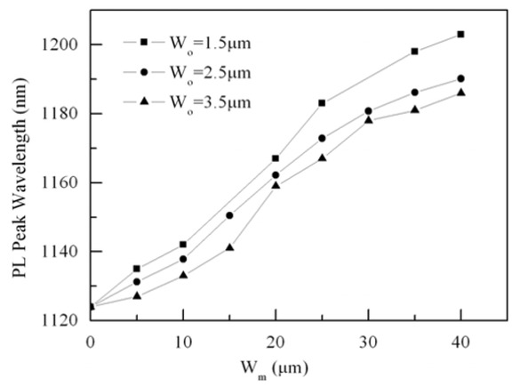
Relationship between maximum wavelength and waveguide thickness.

2.3 Pseudo-limit problems in electromagnetic radiation

When only one scattering of sunlight is considered, the equation of transmission of light in a plane parallel atmosphere can be simplified to the following linear equation:

(7) μ d I ( τ , μ , ϕ ) d τ = − I ( τ , μ , ϕ ) + ω 4 π Π F 0 ⋅ exp ⁡ ( − τ μ 0 ) ∗ P ( τ , μ , ϕ , μ 0 , ϕ 0 ) .

Here the first term on the right side is the direct extinction effect, and the second term is the radiation enhancement source function caused by the single scattering (i.e., the primary scattering of direct sunlight) process. μ₀ and μ are the cosine values of the angle of the solar incident radiation and the zenith angle of the outgoing radiation, respectively, which are positive to the bottom and negative to the upper. ϕ₀ and ϕ are the azimuths of the incident radiation and the outgoing radiation, respectively. τ is the optical thickness, and I is the radiation intensity. ω is the single scattering albedo, P is the single scattering phase function, and Π_F₀ is the extraterrestrial solar radiant flux [4]. The relationship between these variables can be shown in an atmospheric radiation transmission model as below:

Figure 2

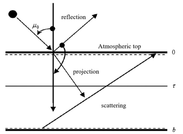
Schematic diagram of atmospheric radiation transmission model.

Assuming that there is no downward diffuse radiant flux at the top of the atmosphere except for direct sunlight, and the diffuse radiant flux at the underlying surface of the atmosphere is totally reflected, then upward radiation at any optical thickness can be easily derived from equation (7).

(8) I ↑ ( τ , μ , ϕ ) = ω P ( τ , μ , ϕ , μ 0 , ϕ 0 ) Π F 0 4 μ 0 μ 0 + μ ⋅ [ exp ⁡ ( − τ μ − τ μ 0 ) − exp ⁡ ( − b μ − b μ 0 ) ]

If τ = 0 is taken, the upward radiation intensity of the atmospheric top or the reflection intensity of the atmospheric top can be expressed as:

(9) I ↑ ( 0 , μ , ϕ ) = ω P ( τ , μ , ϕ , μ 0 , ϕ 0 ) Π F 0 4 μ 0 μ 0 + μ ⋅ [ 1 − exp ⁡ ( − b μ − b μ 0 ) ]

According to the above formula, first let the observation direction approach the horizontal direction μ ⇒ 0 (faster), and then let the sun direction approach the horizontal direction μ₀ → 0 (slower), then the limit expression of the single scattering intensity when (μ, μ₀) → (0, 0) can be obtained as:

(10) lim μ ⇒ 0 , μ 0 → 0 I ↑ ( 0 , μ , ϕ ) = ω P ( τ , μ , ϕ , μ 0 , ϕ 0 ) Π F 0 4 = η

If the sun direction is first approached to the horizontal direction μ₀ ⇒ 0 (faster) and then the observation direction is closer to the horizontal direction μ → 0 (slower), the limit expression for the single scattering intensity at which (μ, μ₀) → (0, 0) can be obtained is:

(11) lim μ → 0 , μ 0 ⇒ 0 I ↑ ( 0 , μ , ϕ ) = 0

If (μ, μ₀) is assumed to be close to (0,0) in an equal ratio, that is, if μ = ξμ₀ → 0 and ξ is any positive numbers, then the limit is:

(12) lim μ = ξ μ 0 → 0 I ↑ ( 0 , μ , ϕ ) = ω P ( τ , μ , ϕ , μ 0 , ϕ 0 ) Π F 0 4 ( ξ + 1 ) = η ξ + 1

Since ξ is a positive value of any value, 1/(ξ + 1) can be any value in [0,1], so the result of the above formula can take any value between [0, ξ]. It can be seen from equations (8)-(12) that when the sun and the observation direction are both close to the horizontal direction, the limit of the atmospheric top reflection radiation is not unique, and its value depends on which (μ, μ₀) first approaches the horizontal direction, or the way these two directions approach the horizontal direction. Hovenier and Stam call it the discontinuity limit and propose to use this discontinuity limit to estimate the optical properties of the planet’s atmosphere [5].

If you look at the mathematical derivation completely, the equations (8)-(12) get the limit is not unique, and the derivation is perfect. But the problem discussed here is a real physical problem, not a purely mathematical one. The conclusions of mathematical equations must be real physical phenomena. The inherent nature of physical phenomena also needs mathematical support. The two cannot be completely separated. Therefore, the results of mathematical deduction need to be verified by physical verification. From the following experiments we can see that the limits obtained by equations (8)-(12) are not the only ones that violate the physical principle of radiative transmission and are a pseudo-limit problem.

3 Physical principles in atmospheric electromagnetic radiation transmission

The relationship between the propagation of the evaporating waveguide and the penetration angle: when the elevation angle of the electric wave in the evaporating waveguide is greater than the penetration angle, the electric wave will pass through the waveguide without waveguide propagation; when the elevation angle is smaller than the penetration angle, the electric wave can be captured by the evaporating waveguide. In turn, waveguide propagation is achieved [6].

To apply the evaporating waveguide for radio wave propagation, the emitted electromagnetic wave is incident on the waveguide at a certain angle. When the incident angle is larger than this angle, the electric wave will penetrate the waveguide, so that the waveguide propagation cannot be performed. This angle is called a critical angle package, or a penetration angle.

When the wavelength of the electromagnetic wave is sufficiently short, the electromagnetic wave propagation can be approximated by the ray theory, as shown in Figure 3. It is assumed that the electromagnetic wave source located in the evaporation waveguide is incident on the upward angle of the electromagnetic wave emitted from the elevation port to a certain height in the waveguide layer (in order to better explain the problem of the refraction of the radio wave, only the refraction at a certain point is considered here, the fact When the upper electromagnetic wave propagates, refraction occurs at every point on the path, and the ray trajectory is a curve instead of a straight line [7]. At this moment, the angle of incidence is i , the angle of refraction is ^ϒ, and the evaporation index n in the large waveguide layer decreases with height. The refraction at this moment must be greater than the angle of incidence. 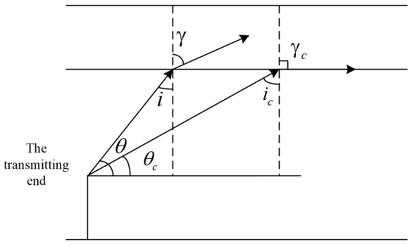When the elevation angle of the emission is lowered to a certain critical elevation angle θ_c, the critical refraction angles γ c = π 2 , and i_c under such condition can be the corresponding critical incident angles. The actual electromagnetic wave is not a straight line but a curve. The basic equation describing its trajectory is the snell formula in the polar coordinate system.

Figure 3

Relationship between electromagnetic wave propagation and penetration angle.

(13) n 1 r 1 c o s θ 1 = n 2 r 2 c o s θ 2

The subscripts 1 and 2 represent the positions of two different heights through which a transmission channel, r₁ = r_e + h ₁ , r₂ = r_e + h₂. r_e is the radius of the earth. If the subscript 1 is the height h₁ of the electromagnetic wave source and the subscript 2 is the height h₂ of any point on the transmission channel, then when ( γ c = π 2 , θ 2 = 0 ) , then the formula (13) becomes:

(14) n 1 ( h 1 + r e ) c o s θ 1 = n 2 ( h 2 + r e )

Further transform above formula into a turbulence form:

(15) Δ n Δ h = − n 1 h ⋅ ( 1 − c o s θ c 1 + Δ h r 1 )

Among them, ᐃn = n₂ − n₁ and ᐃh = h₂ − h₁

By linearly expanding cosθ_c and 1 + Δ h r 1 in Taylor series and ignoring the high order small quantity, the relationship between the critical elevation angle and the refractive index gradient of the evaporation waveguide can be derived as follows:

(16) Δ n Δ h = − n 1 [ 1 r 1 + θ c 2 2 ( 1 Δ h − 1 r 1 ) ]

Then the critical elevation angle θ_c is:

(17) θ c = − 2 ( Δ n Δ h n 1 + 1 r 1 ) ⋅ Δ h = − 2 ( Δ n × 10 − 6 Δ h n 1 + 1 r 1 ) ⋅ Δ h

From the relationship between the refractive index n and the corrected refractive index m, we can get:

(18) Δ n = Δ m c − Δ h r e × 10 6

Since r₁ ≫ h, n₁ ≈ 1, where h represents the height of the evaporating waveguide, |Δm_c| is the difference between the corrected refractive index at the height of the source and the height of the top of the waveguide. For the surface waveguide (evaporation waveguide), if the electromagnetic wave emission source is located on the ground (sea surface), and the radio wave is refracted downward at the top of the waveguide, when there is no foundation layer in the waveguide layer or the thickness of the base layer is thin, the formula (18) can be The approximate simplification is: then the above formula can be approximated as:

(19) θ c ≈ − 2 × 10 − 6 h ⋅ d m d h = − 2 × 10 − 6 ⋅ Δ m

Where h is the thickness of the waveguide. Through analysis, it is obtained that: firstly, the thicker the thickness of the evaporating waveguide, the greater the upper limit of the range of electromagnetic wave emission angles at which the waveguide can be formed; secondly, the stronger the intensity of the evaporating waveguide, the greater the upper limit of the range of electromagnetic wave emission angles at which the waveguide can be propagated. Obviously, when the emission elevation angle is less than the critical elevation angle θ_c, the electromagnetic waves will be able to form waveguide propagation.

4 Mathematical principles in the transmission of electromagnetic radiation

The Snell’s law for a spherically layered atmosphere can be represented by the following picture. Based on Snell’s law, the radio wave propagation trajectory can be easily obtained by combining the initial radio wave emission conditions and the corresponding refractive index profile. As shown in Figure 4, T is the position of the emission source, θ₀ is the initial exit elevation angle of the radio wave, and the distance x on the ground can be used in the case of the refractive index n₀ at the transmitting end and the distances r₀ and cosθ₀ from the transmitting end to the center of the earth. The functional relationship with height h represents the trajectory equation of the ray. Now derive the corresponding trajectory equation.

Figure 4

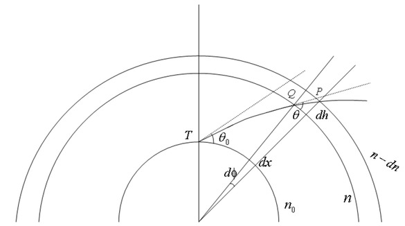
Snell principle.

It can be seen from Figure 4 that on the ray, the corresponding coordinates of Q are x and h. When moving from point Q to point P, the corresponding changes in radius r and height h are:

(20) d r = d h = r d ϕ ⋅ t a n θ

Where dϕ is the change in the angle between the geocentric and:

(21) d ϕ = d x r e

Where dx is the change in ground distance x. Substituting the above formula into equation (21), and r = r_e + h. By integrating the above formula, the projection distance x of the ray on the ground at height h is:

(22) x = ∫ 0 h c o t θ 1 + h r e d h

By substituting (22) with (20) and (21), and considering r 0 = r e + h 0 and r = r e + h , it is tranformed to:

(23) x = ∫ 0 h r e r e + h ( r e + h 0 ) n 0 c o s θ 0 n 2 ( r e + h ) 2 − [ ( r e + h 0 ) n 0 c o s θ 0 ] 2 d h

The physical meaning of each parameter in the formula is: x is the horizontal distance from the point to the transmitting end on the ray, h is the altitude of the point on the ray, h₀ is the altitude of the ray emitting end, r_e is the radius of the earth, and θ₀ is the initial launching angle, n₀ and n is the atmospheric refractive index of h₀ and h respectively.

The denominator root of the integrand of the above formula is subtracted from two very close values. When the elevation angle is small, the error of the calculation result is large, and even the unreasonable case of negative after subtraction can be trapped by the atmospheric waveguide. The initial elevation angle of the obtained ray is generally near the zero degree angle, so the calculation accuracy is improved at a low elevation angle. It is common practice to replace cos²θ₀ with 1 − sin²θ₀ and expand and recombine the items to obtain a continuous calculation formula suitable for the waveguide environment:

(24) x = ∫ 0 h r e r e + h ( r e + h 0 ) n 0 c o s θ 0 a r 0 2 + b r e + c d h

4.1 Taylor expansion approximation

Based on Snell’s law, we can obtain the ray equation (discrete) by Taylor’s second-order approximation. This algorithm judges the next direction by the elevation angle of the previous step in the ray propagation process, so that the program achieves the applicability.

(25) n 0 ( r e + h 0 ) c o s θ 0 = n ( r e + h ) c o s θ

The above formula is the form of snell’s law under the flat ground, and the earth is equivalent to a flat ground. In this case, the problem of handling the atmospheric waveguide is more convenient. Since the angle between the ray and the horizontal boundary of the waveguide is generally small when the waveguide is formed, and the corrected refractive index of the lower atmosphere is close to 1, the second-order approximation to (25) by Taylor seires is made as below:

(26) m ( h 2 ) − m ( h 1 ) = Δ m ≈ θ 2 2 − θ 1 2 2

(27) θ 2 = θ 1 2 − 2 Δ m

Here (θ₁, θ₂) is the elevation angle of the ray at the height (h₁, h₂), and the unit takes the arc (rad).

4.2 Ray Tracing Discrete Algorithm in Waveguide Environment

For the radio wave propagation of the low elevation angle ( − 3 ≤ 3 o ) in the waveguide, the Taylor approximation mode can be used as the tracking algorithm to calculate the hop distance, and for the high elevation angle wave propagation, the integration mode can be used. Here we introduce the ray discrete tracking algorithm under the small elevation angle, namely the Taylor approximation mode.

As mentioned above, under small elevation angles, two situations must occur: first, the radio wave rays whose initial elevation angle is smaller than the limit angle will occur at a position smaller than the waveguide height based on the trapping effect of the super-refracting layer. Rotating, bending to the ground, and then reflecting on the ground, in the form of bounce to achieve over-the-horizon waveguide propagation in the waveguide layer; second, the initial wave angle is greater than the limit angle of the radio wave at the top of the waveguide, the elevation angle is still greater than zero, and then out The waveguide layer propagates normally. The propagation situation in the analog waveguide is actually a very complicated process. Here, using the approximation formula, the feature quantities dh_i, θ_i, h_i, x_i, g_i, m_i describing the step process is obtained, where dh_i represents the height step of the ray from the i th step to the i + 1 th step, and the ray is non-rotating. When the ground is not touched, the value is determined by the density of the given section, and a fixed step dh is set as the reference value. θ_i is the elevation angle of the ray during the i th step at the corresponding height h_i and the horizontal distance x_i from the emission end. m_i and g_i respectively represents the corrected refractive index and gradient at h_i. In above algorithm, the ray propagation is judged mainly by the change of the elevation angle. The ray propagation direction is classified according to the propagation elevation angle θ_i of each step, and then the position of the ray at the i + 1 step is calculated. Therefore, at the initial elevation angle, the antenna is known. The calculation can be performed under the conditions of the position and the atmospheric correction refractive index profile.

If the transmission at a high elevation angle is considered, since the waveguide propagation limit angle does not exceed 1^∘, the beam will surely pass through the waveguide, and the rotation is not required in the calculation, so the corresponding situation is much simpler. At the same time, due to the poor accuracy of the elevation angle Taylor algorithm, the integration mode is still used, and the stepping algorithm is also adopted.

Considering the relationship between m and n. The integral equation (23) about x can be estimated by an one-order numerical discretization:

(28) x i + 1 = x i ± r e r e + h i + 1 m c o s θ i d h i m i + 1 2 − ( m i c o s θ i ) 2

The ± sign in equation (28) is positive when θ_i > 3^∘, and negative when θ_i < 3^∘ (except when bottoming out). The values of h_i₊₁ and dh_i at the situation when touching the ground are the same as those shown in the above classification, and will not be described here.

5 Conclusion

In the general solution of atmospheric radiation transmission, it is often assumed that the atmosphere is in the local thermodynamic equilibrium state, thus requiring the atmosphere to be a dense atmosphere. The energy conversion caused by collisions between atmospheric molecules is much faster than any other method, and the instantaneous recovery factor can be recovered. Offset due to external forces such as radiation. This dense atmospheric model assumes that there is a rigid boundary at the top of the atmosphere, so that atmospheric optical parameters such as refractive index is abruptly changed at the top of the atmosphere. When sunlight is incident on this interface, part of it is reflected back into space, and part of it passes through the interface into the atmosphere. The specific value is determined by the Fresnel equation. Since the refractive index of the entire atmosphere is very close to the vacuum, the Fresnel refractive index is almost 100% for observations with an angle of less than 75^∘, that is, when the solar zenith angle is less than 75^∘ (this is also the effective range of the plane parallel atmosphere mode). Almost all of the sunlight passes through this boundary into the atmosphere. Therefore, in the conventional atmospheric radiation transmission mode, the Fresnel equation is often ignored and does not cause unacceptable errors. However, when the sun and the observation zenith angle are large, Fresnel must be introduced into the atmospheric radiation transmission mode as a boundary equation, otherwise it will lead to erroneous conclusions.

Acknowledgement

This work was supported in part by the Scientific Foundation of Education Department of Hunan Province under Grant 18B569.

References

[1] Murua A., Sanz-Serna J. M., Vibrational resonance: a study with high-order word-series averaging, Applied Mathematics and Nonlinear Sciences, 2018, 1(1), 239-246.10.21042/AMNS.2016.1.00018Search in Google Scholar

[2] Chen Long, Xia Xintao, Zheng Haotian, Qiu Ming, Friction Torque Behavior as a Function of Actual Contact Angle in Four-point-contact Ball Bearing, Applied Mathematics and Nonlinear Sciences, 2016, 1(1):53-6410.21042/AMNS.2016.1.00005Search in Google Scholar

[3] Smolkin E., Numerical method for electromagnetic wave propagation problem in a cylindrical inhomogeneous metal dielectric waveguiding structures, Mathematical Modelling & Analysis, 2017, 22(3): 271-282.10.3846/13926292.2017.1306809Search in Google Scholar

[4] Calandrav H., Gratton S., Lago R., Vasseur X., Carvalho L. M., A modified block flexible gmres method with deflation at each iteration for the solution of non-hermitian linear systems with multiple right-hand sides, Siam Journal on Scientific Computing, 2016, 35(5): 345-367.Search in Google Scholar

[5] Uchida T., Linear perturbations in force-free black hole magnetospheres — ii: wave propagation, Monthly Notices of the Royal Astronomical Society, 2018, 291(1), 125-144.10.1093/mnras/291.1.125Search in Google Scholar

[6] Ylä-Oijala P., Koivumäki P., Järvenpää S., Hybrid multilevel fast multipole algorithm—physical optics for impedance surfaces, IEEE Transactions on Antennas & Propagation, 2016, 64(12), 5475-5478.10.1109/TAP.2016.2606570Search in Google Scholar

[7] Smolkin E., Valovik D.V., Coupled electromagnetic wave propagation in a cylindrical dielectric waveguide filled with kerr medium: nonlinear effects, Optica Acta International Journal of Optics,2016, 64(4), 396-406.10.1080/09500340.2016.1240252Search in Google Scholar

Received: 2019-08-20

Accepted: 2019-12-03

Published Online: 2019-12-31

This work is licensed under the Creative Commons Attribution 4.0 International License.

Articles in the same Issue

https://doi.org/10.1515/phys-2019-0098

Keywords for this article

radiative transmission; local thermodynamic equilibrium; atmospheric optics; Snell’s law

Creative Commons

BY 4.0