Idea of multi cohesive areas - foundation, current status and perspective

1 Introduction

The idea of multi – cohesive areas (MCA) [1, 2] gives a new image to the quantum particles mass. This model contains a group of particles that have the properties of dark matter. There are two most established ways of explaining this phenomena. Those are the modified gravity theorems in the frame of MOND and changes in General Relativity [71] and searching for a new type of particles [3, 4, 5]. However, studies made in [6] favor the latter. Moreover, in [7] it is proved that even if a group of modifications is made to gravity, substantial DM is still needed. On the other hand, popular models based on DM as particles, like WIMPs or AXIOMS, also do not yield any significant outcomes [4, 5, 8, 9, 10, 11, 12]. This situation generates the need for a new, testable idea. MCA is a response to such a need.

The current status of this idea from theoretical and experimental perspective will be presented. Starting point will be presenting the motivation behind MCA creation. Next, its foundations and the main result, which is a new geometrical model of quantum particle mass. This model was obtained by reinterpreting the Heisenberg principle from momentum and location (HPML). generalization of this reinterpretation will be done and by doing that it will be shown that in MCA’s image, HPML is unified with the existence of the maximum speed of energy propagation c - introduced by the special theory of relativity (STR) [13]. The same will be done for energy - time uncertainty relation (HPET). By doing that, the same physical ground to both HPML and HPET will be given. All of that are new results in current MCA’s development.

The purpose for all of that is placing MCA’s foundation on solid grounds and by doing that revealing what change has to be made in its further development. As it will turn out the spectrum of this change contains a new image of fields and particles, a new image of time and a change in the HPML and HPET interpretation. Such a change means no less than a change of paradigm [14]. But, since theories which create this paradigm cannot explain the current experimental data on DM and DE phenomena as MCA does, then this change seems to be necessary.

In the frame of experimental data, one of the most unique MCA’s results is the prediction that DM particle creation probability gets bigger with the bigger initial number of fermions taking part in a single collision act [2]. The importance of this result lies not only in the explanation of the lack of DM signals in LHC [1, 2, 3, 4, 5], but also in the possibility of DM creation from fermions particle. Namely, by this process it will be able to “disappear” things by changing them into DM.

Moreover, this result from astrophysical perspective will be investigated. At that scale, the second most important MCA result – the source of dark energy (DE) [15] will also be introduced. By using CPT symmetry it will be proved, that MCA’s DM antimatter has a negative mass, which is a source of a repulsive force, which in turn can explain the DE phenomenon [16, 17, 18]. This is another new result in current MCA development. Such a new result is also obtaining the stability of a negative mass, by using mass (M), parity (P) and time (T) symmetry. A prove, that such stability is needed is presented in this work. Moreover, it will be proved, that the repulsive force between MCA’s DM and its antiparticle, can explain the lack of DM annihilation signals [4, 5, 19, 20, 21] and can point out where such signals should be looking for. It will be shown that, all of those results not only explain the current experimental data, but also make predictions. However, those predictions are not precise yet. For example, according to the mentioned MCA’s result, probability of DM particle creation gets bigger with the initial number of fermions taking part in a single collision act [2]. But, this does not tell us how many fermions have to be used to create DM. Such a lack of preciseness is the main reason for which MCA on this stage cannot yet be treated as a theory. However, this is where further experimental MCA’s verification can by useful. Taking that a theory should be calibrated toward experimental data, never in the opposite direction, can be stated that further experimental MCA verification could create building blocks for creating a theory from them. It is a quite beautiful perspective when experiments on both micro and cosmic scale complement and support each other.

However, having those building blocks would be useless, without a solid theoretical frame. For that reason, to make a theory from MCA, alongside with experimental verification, theoretical supplementation has to be made. The goal of this work is to create the first step to doing so. It will be done by showing tools for further MCA development and the direction for it. As it turns out this direction is the theory of unification of all known interactions. It is so, because as it will be proven, MCA’s DM interacts only via gravity. But, by the fact that MCA’s mass model contains also visible particles – described in the frame of the Standard Model (SM) [22, 23] - the new image of similarities between gravity and SM interactions will be pointed ou. That will be a starting point to pave a new road to combining all interactions, for which MCA can be a base. The fact, that already on this stage MCA, gives explanation to the current DM and DE phenomena is a proof that this theory will be fruitful. The fact that other DM models and ideas of unification of all interactions do not yield any significance outcomes is a proof that this theory is needed.

This work is structured as follows: in the next section, the motivation behind MCA’ creation and its foundation and main result are presented. Next, the MCA containing DM and DE is proven. Then, HPML and HPET are generalized. It will be used in the section, where the possibilities of experimental MCA’s verification will be presented.

2 Motivation

The motivational question behind the MCA’s creation was - is quantum particle mass built by more elementary quantities, which means, that it is something emergent [1, 2]? Below is the reasoning for this question.

Quantum mechanics (QM) in its established form was born by using de Broglie hypothesis on the wave nature of particle mass. In this hypothesis, it was assumed, that some wave is associated with the mass of particles [24]. But, what kind of wave it is, was not explained. Nevertheless, this hypothesis was used by Schrodinger in his formalism of quantization as eigenvalue problem [25, 26]. The key factor of this formalism is the Schrodinger equation, which can be obtained in analogical way as classical Hamilton – Jacobi equation but instead of using derivatives of an action function, QM’s operators of energy and momentum are used [27]. It is mentioned to point out, that this formalism does not change the interpretation of mass m from what it is in classical mechanics. It just puts m to Hamiltonian operator without changing its physical interpretation. Thus, m in QM’s Hamiltonian is the same as m in classical Hamiltonian - scalar quantity with inertia m.

Therefore, Schrodinger formalism and object that it uses – the waves from de Brogile hypothesis - does not tell what mis. It seems quite disturbing if it is taken that QM became a foundation for particle physics. On the other hand, from STR it is known that mis a form of energy [13, 28, 29]. These considerations led to the mentioned question.

But, these considerations also point out how an answer was found to this question. Since, as was mentioned, Schrodinger equation describes the classical mass, thus in search for the nature of quantum particle mass, other part of QM has to be used. The part which is truly and only quantum. Such part is the Heisenberg principle. It is so, because this principle does not have its analogy in classical mechanics [24, 26, 30]. It exists only in QM. Also, it describes momentum which is directly related to mass. For that reason, the search for an answer was due to focus on the reinterpretation of HPML. Assuming that HPML is an intrinsic property of nature [27, 31], its reinterpretation is allowed. Such reinterpretations are not new in physics. For example, gravitational interaction, since it is a property of nature itself, has been reinterpreted by general theory of relativity (GR) as curvature of time – space. Before that, this interaction was interpreted in the form of vector forces [29, 32].

Thus, the answer to MCA’s motivational question was obtained by reinterpretation of HPML. But, in this reinterpretation, the mentioned mass energy equivalence could not be omitted. Since foundation for this equivalence is the Lorentz invariance [29, 33], thus this reinterpretation and the entire MCA is based on mathematical apparatus for which Lorentz invariance is also fundamental – the conformal algebra.

This section can now be summarized : the motivational question behind the MCA creation was - is quantum particle mass something emergent, which means it is combined of more elementary quantities? Answer to that question was found by the reinterpretation of HPML using the conformal algebra. It is time to present the result of this answer and the way by which it was found.

3 MCA’s foundation and main result

As mentioned in the previous section, in searching for the answer to such motivational question, mass energy equivalence could not be omitted. Foundation for this equivalence is Lorentz invariance. For that reason, MCA’s foundation is a mathematical apparatus which was born from this invariance – the conformal algebra [34, 35].

MCA uses two-dimensional version of it [36]. This mathematical apparatus allows describing the 3-dimensional space of the physical observation R – homeomorphic to Minkowski space [37] - by the 2-dimensional complex plane C [36, 37]. It is so because of the stereographical mapping between Riemann sphere S, isomorphic to R, and complex plane C. This mapping is bijective and conformal [37]. The isomorphism between these three spaces can be pictured as follows:

Moreover, in this theory, Lorentz action in the space of the physical observations R is substituted by the homographic mapping at complex plane C

where a, b, c, d are the complex numbers. Homeomorphism of these groups can be pictured similar to (1), as

a sphere S

Conformality of the homographic mapping and stereographicalmapping, as it turn out, is very important in MCA. This conformality is responsible for the fact that circles in MCA are universal – they are the same for different inertial observers [37]. Also, circles on C plane are circles or a straight line on the R real space. Moreover, since stereographical mapping is bijective [37], then circles on C plane are circles in R. All of that is in the frame of conformal algebra in two dimensions. However, this theory is usually used in building a field theory [34, 35]. Such a two-dimensional conformal field theory (like any other field theory) is determined by its space of states and the collection of its correlation functions [34]. MCA is not defined by such a space and functions. Instead, MCAis determined by its assumptions. Reason for which MCA does not operate in the frame of fields, will be explained later.

First MCA assumption is that derivative of (2) function is the speed of light at C plane

Taking the above-mentioned fact that 3-dimensional real space R corresponds to the C plane, where (2) is defined, and the fact that homomorphism of this spaces is bijective, it can be stated that speed of light corresponds also to the 3-dimensional real space of physical observations R.

According to vector interpretation, the derivative of the complex function defines a vector field at the complex plane [36, 38]. Thus, it can be stated that this assumption introduced the field of the light speed vector. Moreover, this derivative (4) is defined in areas where Cauchy – Riemann conditions are true

where the fact that (2) function can be written by using the function of real variables φ(x,y), ψ (x,y)was used [36, 38].

Moreover, according to complex analysis and differential geometry, a derivative (4) exists only in areas in which [36, 38]:

where

C-R conditions (5) are equivalent to (7) and (8), if taking (4) into consideration [39]. In other words, (5) can be substituted by (7) and (8). Indeed, using the fact that assumption (4) introduces a field of the light speed at C:

Then, using (5), (9) and (10), C-R equations are obtained

Taking now a differential of (5) respecting (11) and (12), obtain (7) and (8), are obtained. From (11) and (12), it can be stated, that functions φ(x,y), ψ (x,y) represent fields on the real plane, which correspond to complex plane C.

Taking the integral from (4):

it can be seen that the real part of this integral equals the circulation of the lights speed vector at the closed curve

and the imaginary part equals the productivity of the source – value of the source of the light speed field

From comparing (14) with (7) and (15) with (8) it can be observed that (14) equals zero when (7) is true, and (15) equals zero when (8) is true [39]. Since in this stage of the MCA’s development, the physical meaning is only had by (14), in the further part of this work (15) and (8) will be omitted.

Summarizing the first MCA’s assumption – it introduced the field of the light speed vector at C plane. Also, alongside with that, two functions of real variables are introduced φ, ψ. Those functions represent fields at the real (x,y) plane, which correspond to the complex plane. First of those fields describes a direction of the light speed vector, and the second represents the value of this field at some point [36, 38, 39]. Thus, those functions show how the field of the light speeds spreads and give the value of the light speed vector at some point. These function satisfied (5) condition as a necessary condition for (4) to exist.

Moreover, this assumption introduced two types of areas. The first one where (7) is true and second one where (7) is not true. From (14) it can be observed that border between these two types of areas is the line of the circulation of the light speed vector. Inside the circulation curve, the area is not holomorphic – (7) is not true and (4) does not exist. Outside the curve, the area is holomorphic – (7) is true and (4) exists. Now, the multi cohesive areas can be explained. It is an area where on a single complex plane C, there are holomorphic and not holomorphic areas, separated by the line of the circulation of the light speed vector Γ.

The second and the last MCA assumption is that energy can be exchanged only in points where (4) function equals zero. In such points, according to conformal algebra, function (2) is not conformal [34, 35, 36, 37]. Those points are called the zero point z_i. To better illustrate this assumption consider the following situation. An observer located at point A sends a light signal to an observer located at point B, using a flashlight. The exchange of the mechanical energy (e.g. energy to press the switch and turn on the flashlight) are omitting and focusing only on two phenomena - creation and annihilation of the photon. First zero point is in A. In point A, energy is exchanged between a flashlight and an electromagnetic field – the creation of a photon. The second zero point is in B, inwhich electromagnetic field transmits the energy to the observer (to the particle belonging to the observer’s body) – the annihilation of the photon.

That is all in the frame of MCA’s assumptions. Let notice, that such assumptions introduce a discreetness in the area where energy can be exchanged, so also where interaction can take place. It is so, because according to MCA’s second assumption, energy can be exchanged only at zero points. Since those points are defined only where function (4) is defined, then it can be stated, that in non-holomorphic areas there are no zero points, so there are no interactions. Thus, as it can be seen, MCA limits the interaction areas by introducing zero points as the only points where energy can be exchanged and non-holomorphic areas, where those points cannot exist.

The existence of areas where interaction cannot take place in string theory led to change of HPML into generalized uncertainty principle (GUP) [40]. Having a different motivation, mentioned in the previous section, MCA also changes HPML. It will be shown now how.

To do that, a proper (4) function for the following situation should be found. The fact that (4) can be written as a Laurent series will be used

Let a free particle with quantum inertial mass m be located at the non-holomorphic area – inside the circulation curve. Let the circulation curve have the shape of a circle, because of the universality of those - the same for different inertial observers. Moreover, let outside circulation, area be fully holomorphic and conformal. Since function (4) is a derivative of a homographic function, only fully holomorphic part in (16) is a₀. So, a₀ ≠ 0 outside the circulation curve. Let a₀ = c be the speed of light in vacuum. To obtain conformality of a holomorphic area, zero points have to be located in non-holomorphic area or at the edge of it - on the circulation curve. It is so, because in zero points, function (2) is not conformal. Thus, to erase the non-conformality from holomorphic area, one have to put zero points at the mentioned location. Taking all this into consideration, plus the fact that, according to MCA’s assumption, (16) has to represent a derivative of a (2) function, it is obtained

for n ≤ −3 and n > 0. Thus, using (17) and (16), it is

It should be noticed that a different way to obtain a holomorphicity of an outside circulation area, is to assume that far from the circulation and particle in it, so when z → ∞, it is V(z) = a₀ = c.

Let now define HPML. MCA’s uncertainties as follows:

where, Δz_i = z_ß+1 − z_i . The reason for such definitions of uncertainties will be explained later. In QM, the product of uncertainties in the case of a free particle equals [1, 26, 30]:

For the t > 0, it can be seen that this turns into HPML

To obtain analogical product with uncertainties defined as (19) and (20) in the case of a free particle located at the circulation curve, zero points in (18) have to be found, to calculate Δz_i in (20). Since, according to MCA’s assumption, zero points z_i are points for which V(z_i) = 0, to find those, have to compare (18) to 0. By doing that, it is obtained:

It should be noticed that for |Γ| ≤ 4πRc

Now, a product of (19) and (20) can be calculate. Using (22), it is obtained

It can be seen that for Γ > 0, HPML is obtained. By comparing (21) with (24), it is:

where m – quantum particle (inertial) mass; h – Planck’s constant, Γ circulation of the light speed vector (circulation); k = ct/Δz_i . Δz_i= z_i+1−z_i.

(25a) is the main MCA’s result. Above equation was theoretically verified by obtaining established mass energy equivalence m = E/c² from it [1]. For the rest mass, k = ct/Δz_i = const = 1. This equivalence between (25a) and m = E/c² is a result of the fact, that both MCA and STR from which m = E/c² was obtained, have the same foundation – Lorentz invariance.

This new model of quantum particle mass (25a), corresponds to the three groups of particles presented in the figure below: First two (from the left) groups of particles were identified as follows:

• Fermions are particles for which |Γ| < 4πRc

• Bosons are particles for which |Γ| = 4πRc

This grouping was done by introducing the total circulation. This quantity, due to Cauchy integral theorem for multi cohesive areas, is equal to the number of all circulations contained in the total circulation [36, 38]. Moreover, as it was proved in [1, 2], this quantity is time constant. Let us call this rule the total circulation symmetry. By applying this rule to the fact that boson can fall apart into fermions, and fermion cannot fall apart into bosons [26, 28], it was stated that bosons have to have bigger value of circulation than fermions. Only then, the process of braking a boson into fermions would not violate the total circulation symmetry rule.

It can be seen in Figure 1 that for a single circulation area, for bosons would be Δz_i = 0. Then, according to (25a), the mass of the boson would be infinity. To omit that, a characteristic of bosons from SM has been used. According to SM, bosons transmit energy, while fermions are constituents of the matter [22, 23, 41]. Thus, bosons transmit energy between fermions. From MCA’s perspective, this transmission is due to distribution of the zero points between two zero points located at the circulation areas of two fermions. Thus, it has to be assumed that the second zero point for boson is located at the different circulation area than the first zero point. To obtain that, it was

Figure 1

MCA’s particles at complex plane C. Zero points are marked with grey dots. As it can be seen, curvature of the lines of the light speed field at the outside part of circulation is generated by the circulation itself [2]

taken that k in (25a) for bosons case is:

It is then:

g(z₁) is a conformal transformation. Location of the first zero point is given by V[g(z₁)] = 0 and the location of the second zero point is given by dg/dz₁ = 0. After that, boson’s mass is no longer infinite. It is graphically presented in [1].

As it can be seen, there is one more group of particles |Γ| > 4πRc. Next section is devoted to it.

4 MCA’s DM and DE model

In this chapter, it will be proven, that the last group of MCA’s particles, for which |Γ| > 4πRc, is a perfect DM candidate [3, 4, 5]. Moreover, it will be shown, that MCA’s DM antiparticles have a negative mass. Such a quantity, as a source of a repulsive action, can explain the DE phenomena [16, 17, 18].

Let start from presenting MCA’s DM model.

5 Generalization of HPML

In this chapter, the link between MCA’s conformal foundation and QM, which is the reinterpretation of HPML, will be bring back. The goal of this chapter is generalization of MCA’s HPML to the cases of all particles and curved space – time. As a result of that, it will be obtained that HPML and analogical uncertainty relation for energy and time (HPET) are unified with the existence of the maximum speed of energy propagation c. This unification is the generalization of HPML (and HPET) to the cases of bosons and curved space time, because rule that c is the maximum speed of energy propagation is true for any particle and any physical system [29]. As it will be also proven, this unification in turn leads to the result that for MCA’s DM sector, reverse HPML and HPET area true. This result in turn, as it will be presented, has a practical side. It will be used to obtain a stability of a negative mass of MCA’s DM antiparticle.

Let start from explaining the choosing suchuncertainties as (19) and (20). To locate a particle, one have to send a signal to the location at which this particle is. Moreover, this signal has to come back to the measuring apparatus. Since, the localization process requires an exchange of energy between the particle and a signal [32], then zero points have to occur. But, according to our assumption, the particle is located inside of the circulation area. For fermions and bosons, zero points do not occur at the inside part of circulation, where the particle is. According to Figure 1, for those kinds of particles, zero points are located at the edge of this area. Thus, since particle is located in this area, and zero points do not occur at this area, which is necessary to locate this particle, it was assumed that uncertainty of location is proportional to the size of this circulation area. Thus, it was assumed that Δx = R, where R is a diameter of a circulation circle. As was mentioned, circles are universal in MCA, they are the same for different inertial observers. This fact, together with the noticing that zero points are located at the circulation circle plus the fact that any product of uncertainties has to obey HPML, have been used to define uncertainty of momentum as (20). With such definitions as (19) and (20), HPML is a consequence of the well-known geometrical fact that diameter length of a circle is no less than the length of its chord

which is presented in the below figure. In other words,

HPML for uncertainties defined as (19) and (20), is obtained from (32).

But, presented HPML is true only for fermions. It is so, because it depends on the fact that two zero points are located at the single circulation circle. Such conditions do not apply to bosons, because in this case, two zero points are located at two circulation circles. Moreover, since MCA’s HPML is purely geometrical and since the only MCA’s quantity is the speed of light which can bend under gravity, then gravitation effect on presented HPML should be studied. It will be seen, that generalization of presented HPML for the case where gravity is on, also generalizes it to the case of bosons.

So, let now turn the gravity on. In MCA it will manifest itself as a curvature of the light speed field. It is so because the curvature of the light speed field means the curvature of the light path. The curvature of the light path means the curvature of the time – space. Everywhere where time-space in curved there is a gravity interaction. All of this is in the frame of the general theory of relativity [29, 37, 43].

Thus, in curved space-time, presented in Figure 2 HPML will not be accurate. It is so, because the line of the circulation curve is bent when gravity is on. HPML based on circle geometry (32) will not fit into this scenario because circulation curve Γ will have a different shape than a circle. This transmission of a shape change, between real space R, in which gravity acts, and complex plane C, is due to conformal nature of the stereographical mapping. It transforms Riemann sphere S, homeomorphic to the real space R, into complex plane C in the way that preserves angles. So, if change of a shape due to gravity in Riemann sphere S occur, it leads to change of an angle between optional two non-parallel straight lines tangents to a circle and that in turn leads to the change of this angle in complex plane C which finally leads to the change of a shape of the circulation curve Γ [36, 37, 38, 39]. It is presented in the figure below:

Figure 2

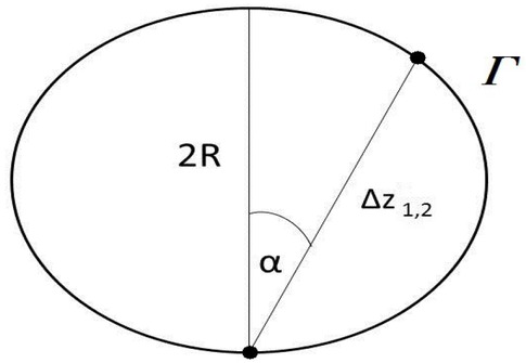
MCA’s HPML as a consequence of the geometrical fact that diameter length of a circle is no less than a length of a distance between zero point, which is a chord of a circle. Zero points are marked as black dots. Circle on which HPML in MCA is defined is the circulation circle Γ

Thus, as it can be seen, a generalization of HPML for the case of curved space – time is needed. However, this generalization should not be less general than MCA’s HPML in the case of fermions. It means precisely, that this generalization should be independent from changing the reference point. In MCA, homographic function (2) is responsible for Lorentz transformation. Thus, this generalization should hold true for any (2) transformation. Let approach to find such a generalization.

According to (9) and (14), the circulation circle on which HPML is defined is one of the lines of field φ [1]. It is so, because the circulation circle is made by the holomorphic area. In holomorphic area function (9) exists and with that function, fields φ, ψ also do.

Therefore, the tools designed to describing a field can be used. Some of those tools are gradient (grad or ∇) and the directional derivative ∂_s. A common relationship of those two is presented in the following figure [38, 39, 48]:

It should be noted, that by using grad and directional derivative to the line of the φ field in shape of the circulation circle, at which HPML from Figure 3 is defined, then

Figure 3

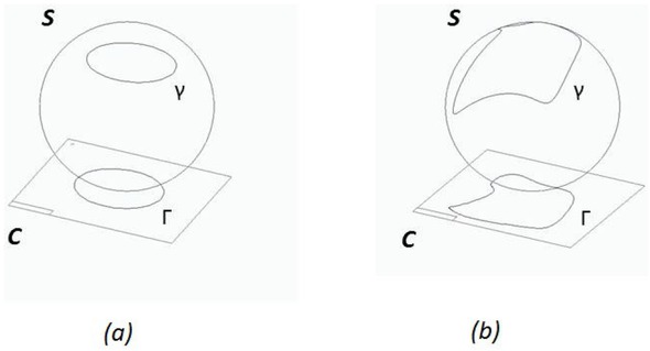
Without gravity (a) circulating circles ϒ at Riemann sphere S, which correspond to 3-dimensional space of the physical observations, are circles at the complex plane C. When gravity is on (b), it bends circulation curve on the Riemann sphere and this bending is transmitted at the complex plane. Thus, circulation curve at complex plane Γ is not a circle anymore

the angle α at Figure 3 equals the angle α at Figure 4. It is then

Figure 4

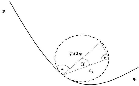
Relationship between grad φ and directional derivative ∂_s. The angle between grad φ and line φ is 90 degree. Presented line of field φ is part of a circulation curve Γ from Figure 3 (b)

From the above:

Gradient (at Figure 4 presented as grad) and directional derivative are the general, geometrical objects. That makes them independent from the conformal transformation (2) of a C plane. Relations between those, presented by (33), are true for any shape of a line of field φ [39, 48]. Therefore, by using these objects, the generality condition mentioned earlier has benn reched.

It can be seen now, that considerations about a special line of the φ field in the shape of the circle, led to connect those geometrical objects with the quantities related to the MCA’s uncertainties. It manifests itself in (33). This trick, as it soon turns out, is the key factor to generalize the HPML in MCA from the case of flat time – space to the case of curved time – space.

According to (9), (6) and (5), it is [1]

Therefore, from (33) and (35) it can be stated, that directional derivative is the speed of light in (optional) direction s:

By introducing (36) the condition for curved time – space was fulfiled. This condition was, as already mentioned, that circulation curve can have a different shape then a circle. For that reason, vector of the lights speed field can change direction on circulation curve and this direction can be optional. That is why (36) was introduced, which manifests the lights speed value at this optional direction. Therefore, it is known that if the gravity is present, one is dealing with the situation where direction of the light speed vector at circulation circle can be optional. The next step is to investigate whether it is also true for the value of the light speed vector at this circulation curve. So, the question is - is there any restriction for |V(z)| on a circulation curve?

In (33) and in Figure 2 there is a distance between two connected zero points |Δz₁,₂|. This fact adds a condition, that on this circulation circle zero points exists. Therefore, one should study a restriction of the lights speed at the circulation circle with connected zero points on it. This connection is through the line of the circulation circle, made by a field φ. If field φ exists between two zero point, then that means that those two zero points are connected by the holomorphic area.Without it, zero point would not be connected. Thus, if one want to learn about the restriction on the light speed at the circulation curve with zero points on it, then what are the restrictions on the line of the light speed that connects two zero points has to be known. It should be notice that specific locations of zero points or a specific line of the light speed vector or direction which those lines should have either was not assumed. It was only assumed the existence of zero points themselves and the existence of a holomorphic area which connects those points. Therefore, this consideration should be independent from direction of the line of the light speed and localization of zero points. For that reason, one study a limitation on |V(z)|, not on |V_S(z)|, because |V(z)| refers to the most general case of connected zero points.

According to the MCA’s assumption, zero points are responsible for energy exchange. Namely, only in those points energy can be exchanged. In MCA, only connection of those points is the line of the light speed field. So, if only in zero points energy can be exchanged and only connection of those points is the line of the light speed, therefore usinge the fact known from STR about maximum speed of energy propagation [29, 37], it can be stated that speed of light on the line which connects two zero points is limited by the light speed in vacuum c. If it were different, then time between the appearance of the first zero point and the second zero point would be shorter then c/d where d is the distance between those points. That would mean, that energy is transmitted on the line of the light speed filed (holomorphic area), that connects those two zero points, faster than speed of light in vacuum, which is in contradiction to STR [29, 37]. For that reason, it has to be taken that speed of light on the line that connects two zero points is limited by the speed of light in vacuum – maximum speed of energy propagation. In other words, zero points are connected only by lines of the light speed field at which |V(z)| ≤ c.

To better picture this, let use the mentioned case of the flashlight and zero point A – creation of the photon, and zero point B – annihilation of the photon. Let take that distance between A and B is d. If the above assumption would be not true, then time between appearing A and B would be less than c/d. That would mean that energy of the photon is transmitted faster than speed of light in vacuum, which is in condration to STR. For that reason, it has to be taken, that on the line of the light speed field (holomorphic area) which connects two zero points, speed of light is limited by the speed of light in vacuum.

So, in a holomorphic area that connects two zero points, the speed of light value cannot be bigger than the speed of light in vacuum:

From above consideration, it can be stated that (37) manifests the rule from STR, that energy cannot be transmitted faster than speed of light in vacuum. Just as this rule is independent from direction of the energy propagation, (37) is independent from direction and a length of the line of the lights speed that connect zero points. Taking (36) and (37) into consideration, it is:

Taking (34), (35), (36) and (38), it is:

Now, using (19) and (20) finally get

According to (40), HPML is true if and only if, the speed of energy propagation is limited be the speed of light in vacuum. Therefore, it can be finnaly stated that in MCA, HPML is unified with the fact known from STR about the maximum speed of energy propagation. It should be noticed, that because of the general formalism that we used in (33), this result is also true for the case of flat time – space. It is so because the relation between gradient and the directional derivative is independent of the shape of the line of the light speed. So, even for the cases where the curvature generated by the gravitational effects can be omitted, this generalization of HPML is still true.

Moreover, this proof is independent from location of two connected zero points. By this characteristic , it can be stated that it refers also to the case of bosons, where location of two connected zero points is not limited to a single circulation. Therefore, it can be finally stated that generalization of HPML to the case of bosons and to the case where gravity is on, leads to unification of HPML with the existence of the maximum speed of energy propagation.

It is important to underline that this generalization does not lead to a new version of HPML, just like it is for GUP [40]. It leads to the state where HPML is nothing more than a manifestation of the existence of the maximum speed of energy propagation, which (40) clearly states. Thus, this result generalizes HPML to the case of bosons and curved space – time, by unifying it with the existence of the maximum speed of energy propagation. Since this rule is true for both bosons and curved space time, and since according to (40), MCA’s HPML is unified with this rule, then it is also true in those cases.

As it will turns out in the next chapter, what seems to be a brutal erasing of HPML as a unique physical rule, touches also HPET – Heisenberg principle for energy and time [26]. By doing that, it puts those two on the same physical ground, which does not exist in any current version of HPET [49].

6 HPET in MCA

In QM, HPML is related to HPET [26, 49]. Having this in mind, it is justified to verify how the result obtained in the previous chapter transmits itself at HPET. As it will be proven, both HPET and HPML are unified with the existence of the maximum speed of energy propagation. Let start from defining the uncertainty of energy ΔE and uncertainty of time Δt.

According to current interpretations, quantities ΔE and Δt in HPET are not uncertainties like Δp and Δx in HPML. ΔE and Δt correspond to some value of energy and time [49, 50]. However, taking that Δx and Δp in QM’s HPML describe value of momentum and location which cannot be simultaneously measured, then Δ in HPML means the same as Δ in HPET - those also define a value of some quantity. Thus, let take that ΔE and Δt describe some value of energy and time.

It is known, that mass is a form of energy. Let use this energy - mass equivalence. It is more justified, if taking that in [1] it was proven that from (25a), m₀ = E/c² can be obtained. Thus, by comparing MCA’s mass model with rest mass from STR, it can be obtained, that:

Since it was assumed that E corresponds to some value of E, study from ΔE to ΔΓ can be transfered

According to MCA’s main result, presented in Figure 1, for visible particles - fermions and bosons - it is:

Dealing with only positive values of Γ, one obtain

Now, using (27), it is:

Then, using (42) and (45) in (44), it is:

It can be seen that limited value of circulation for visible particles - fermions and bosons - is responsible for HPET in MCA. Let now identify what creates this limit.

Circulation is created by close integral of the light speed vector at circulation curve.

There are two components which create circulation, hence which affect its value and which can change independently in time. It is the speed of the light speed vector at the circulation curve and the shape of a circulation curve. But separately, those two components equal zero if taking integral of those at closed curve. Indeed, an integral of a closed curve is [38, 39]:

And in the case of speed at the circulation curve, it is:

where the Stoke formula where, df is the directed area of a complex plane has been used. Above is due to the fact that [38, 39]

Thus, as it can be seen, to verify the limit of circulation (44), one cannot use circulation quantity directly. Thus, a different approach have to be taken.

According to MCA’s assumption, (18) equation presents the speed of light field. Through its construction, it can be stated that there are two distinguished areas on which this field exists. It is the circulation curve and outside part of the circulation curve. Value of the field at the circulation curve relative to the value of the light speed field at the outside part is what distinguish three groups of circulations, presented in Figure 1. Value of the light speed field at the outside part equals c. Therefore, it can be stated, that what separates three MCA’s value of circulation, is the speed of the light at the circulation curve relative to c. There is one more quantity, for which value depends directly on the value of the speed relative to c. It is the relative distance (28).

Thus, to find the source of limitation of the circulation (44), one can use considerations made in 4.1 chapter, where the value of the relative distance with the value of circulation was comined. Using (28) it can be stated that the value of the light speed for circulation of bosons and fermions is less that c, because ds² ≥ 0 for those circulations, according to (28) and (23). For |Γ| > 4πRc speed of light at circulation curve is bigger than c, because in that area ds² < 0.

Thus, it can be stated that what separates |Γ| ≤ 4πRc from |Γ| > 4πRc is the speed of light value at the circulation curve. For inequality from which MCA’s HPET was obtained (43), this value is less than c. For |Γ| > 4πRc this value is bigger than c. Therefore, it can be stated that what limits the circulation value in (43) is the speed of light in vacuum c. Without this limitation there would be no inequality (43), from which MCA’s HPET was obtained.

According to this result, source of HPET is the existence of the maximum speed at the circulation curve c. Since this result is the same as obtained in the previous chapter, it can be finally stated that source for both HPET and HPML is the existence of a maximum speed of energy propagation, which can be schematically pictured as follows:

It should be noticed that in every part of this proof in this chapter and previous one, it the case above c has not been excluded. Moreover, from (40) it can be stated, that one can reverse it and obtain:

The same is for HPET. If instead (43), one use the reversed version of it, which is |Γ| > 4πRc, one obtain ΔEΔt < ℏ/2. Therefore, it can be stated that above c border, reverse HPET and HPML are true. Since, as was proved in the 4^th chapter, the above c border area is the area created by the circulation of the DM particle, it can be finally stated that for MCA’s DM sector, reverse HPML and HPET are true. As it will be seen in the next chapter, this statement has a practical value. Namely, a stability of MCA’s negative mass from it can be obtained.

Figure 5

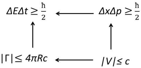
In MCA, HPET can be obtained from the existence of the maximum speed of energy propagation |V| ≤ c, through MCA’s main result. Because in order to obtain HPML from |V| ≤ c only the MCA’s assumption has been used, then it can be stated that |V| ≤ c is related with HPML more directly than |V| ≤ c with HPET

7 Experimental verification

The previous chapter was the last one where theoretical side of MCA was presented. It is time to present its experimental side. Namely, how MCA explains experimental data on DM phenomena on both micro and cosmic scale will be veryfied. Moreover, MCA’s prediction for further experimental verification will be presented. Starting point for that will be pointing out the differences between MCA’s DM and other DM particle models [3, 4]. This way, will be preparing to face the changes, necessary to adapt in MCA’s considering and further development.

It is important to notice that, already at this stage, differences between MCA’s DM model and others popular models, like WIMP, can be seen. Probably the most important difference is that according to MCA’s, DM interacts only via gravity, while WIMPS interact also by other interactions [4, 5]. Other, no less important, difference is that according to popular DM models, those particles can be created by collision of two fermions. For that reason, there are searches for DM signal at LHC, where a pair of protons collide [2, 4, 51]. But, according to MCA’s DM model, probability of DM particle creation gets bigger with the initial number of fermions taking part in a single collision act. This difference will be presented and discussed in the first way. The last difference that will be discussed here is the fact that MCA’s DM antimatter has a negative mass. WIMP or AXION models does not introduce negative mass [4, 5, 9]. Let start from presenting MCA’s prediction on DM creation and through that, direct detection of it [2, 3, 4].

It is known that particles can be created in the collisions of the other particles. Those processes are ruled by conservatory principles. In MCA, such a principle also exists - total circulation symmetry, first introduced in section 3. According to this rule, total circulation of a system is constant in time. Total circulation of a system equals the sum of all circulation that are contained in the total circulation [2]. Since in MCA, circulation creates particles, this rule can be used in MCA’s particles creation process.

By doing that, it was proved, that probability of DM particle creation is proportional to the number of fermions taking part in a single collision act [2]. In other words - probability of MCA’s DM particle creation in collisions of three fermions is bigger than in collisions of two fermions.

To prove this result in a concise way, let notice that MCA’s visible particles (fermions and bosons) are grouped like particles in SM - by the value of the spin [22, 23]. Fermions, particles with the lowest value of spin in SM, in MCA are particles with the lowest value of the circulation. Then, there are bosons, with spin value bigger than fermions, just as it is for MCA’s circulation. Both spin and circulation can be used to describe a value of the total spin or total circulation of a system of particles. Both those total quantities are conserved. Thus, it can be seen see that there is an analogy between MCA’s total circulation and SM’s total spin. But, in MCA there is one more group of particles. Using the analogy between the total spin and total circulation of a system to this group, it can be stated that just in a way by which a single boson falls apart into two fermions, thus a single DM particle, since it has a bigger value of circulation than boson, falls apart into more than two fermions. If it would be different, then the total circulation conservatory rule – analogical to conservatory of the total spin rule – would be violated. It is so, because a system with two fermions could have a smaller total circulation value than a system of a single DM particle. This total circulation conservatory rule allows the opposite process to also be possible – the creation of DM by collision of the proper number of fermions. Thus, assuming that DM particles fall apart into three fermions, then according to the circulation conservatory rule, this proper number is three and that number of fermions is necessary to obtain a DM particle in a single collision act. In [2] fully prove of this statement is presented.

The result, that DM creation probability gets bigger with the number of fermions taking part in a single collision act has been used so far to explain the lack of DM signals at LHC [2]. But, such collisions can take place also on a cosmic scale [23, 52]. Thus, it is proper to use this result in the context of the current astrophysics experimental data.

Namely, taking that probability of more than two fermions participating in a single collision act is bigger in areas where visible matter density is bigger, than it can be stated that DM density in some area is proportional to the visible matter density in such area. Behind this result is an assumption that DM does not leave the near area in which it is created at a fast pace. Since, MCA’s DM only interacts via gravity - the weakest force of them all [23, 52] - then it can be stated that this assumption is quite reasonable. However, at this stage of MCA’s development one cannot give any precise values to make this result accurate. It is not even known how many fermions in a single collision act are necessary to create DM. The fact that by collision of two fermions, no signal of DM has been found [2, 3, 4], suggest that at least three fermions are necessary. In other words - MCA only tells that probability of DM creation in fermions collision gets bigger with the initial number of fermions taking part in a single collision act. But, it does not tell how many fermions are required to make DM. More-over, other conservatory rules that could be true for DM sector have not been taken into consideration. For example, in [53] it is studied that DM carries some electric charge. Assuming, that in the further study on DM creation, conservation of this quantity has to be also taken into consideration. Another quantity, crucial to reach preciseness, which is not defined exactly in MCA, is the value of mass of MCA’s DM particle. It can only be estimated as lighter than that of fermions. It is so, because if one take that for free particle k = 1, as is proved in [1], it can be sees that since DM particle has the biggest value of circulation, then according to (25a), those particles have the lowest rest mass.

It should be noticed that our proof of this result depends on circulation symmetry in a single collision process. Thus, even if in collision of a pair of nuclei, more than two fermions take part, DM creation is still less probable, then in collision of three fermions in a single collision act. It is so, because when two nuclei collide, then number of a collision of a pair nuclei is far more greater than fermions taking part in a collision of a nuclei (participants) [54]. Taking all what was discussed on DM creation probability, the schematic verification of this result can be pictured as follows:

Figure 6

MCA’s model of DM particle creation. At part a) pair of electrons e- and pair of protons p+ accelerated by two linear accelerators perpendicular to each other, collide at marked central point. Such a collision generates DM particle and visible particle F to obtain energy – momentum equivalence, which is presented at b) part. Such a DM creation would be noticed by missing transferred energy and momentum [55]

As it can be seen, two linear particle accelerators was used. It is so, because as was mentioned, DM free particle mass has been estimated as smaller than free fermion particle mass, thus energy enough to create DM particle should be smaller than to create a free fermion. Thus, searching for DM creation should be started from using linear particle accelerators, as accelerators which generate relatively small value of energy collisions relative to other accelerators i.e. synchrotrons [52].

Going back to the astronomical scale. The fact is that at this stage assign a precise value to DM mass cannot be done. Since, knowing the value of mass is crucial to make any precise astronomical prediction, it has to be stated that presented result on DM density is not precise. But more light can be shed by experimental data on DM density in the Solar System [56, 57, 58]. Since according to those results, DM density in the Solar System is low, then taking result on DM density, one can state that DM density should be bigger in the areas where visible matter density is bigger that it is in the Solar System.

In the frame of matter density on a cosmic scale, there is an unsolved problem. The core - cusp controversy or the core - cusp problem reflects the persistent difference between simulations and observations on the mass distribution in the galaxies [59]. It includes also DM. In [16], it was proved that a negative mass can solve this problem. Such kind of mass was introduced in 4.2 Section. This is the first issue which can be explained by negative DM mass from MCA’s model. The second one is related with the annihilation process.

As was proved, negative mass in MCA exists only in MCA’s DM antimatter sector. Since, DM particle has a positive mass, then it can be stated that a pair of a free DM particle and a corresponding antiparticle, since they have the same absolute value of mass, creates a gravitational dipole [16, 17]. It is a pair of two particles, one with positive mass, one with a negative mass, accelerating in a common direction, the negative mass following the positive one. Thus, because as was mentioned, MCA’s DM is only available for gravitational forces, then it can be stated that such a pair does not collide. It is so, because since they are accelerating in the common direction, they do not move towards each other, which is crucial to collide. Taking that collision of a particle and a corresponding antiparticle is necessary for an annihilation process, then it can be finally stated, that MCA’s free pair of particle and corresponding antiparticle does not anihilate. That could explain the lack of confirmed DM annihilation sightings [19, 20, 21]. But, this result is only true for a free pair of DM particle and DM antiparticle that interact only witch each other. Therefore, one more result from this model can be obtained – DMannihilation signals should be looked for in areas where the gravitational field acts it the way that gravitational dipole could collide. In other words – such signals should be found in areas where external gravitational forces can overcome inert gravitational repulsive force between gravitational dipole. These external gravitational forces should act in the way which allows for DM particles, that create a gravitational dipole, to collide into each other.

Nevertheless, once again, at this stage one cannot put any numbers behind those results to make them more precise. To fix this in some way, based only on CPT symmetry, and on a possible number of positive and negative signs of time and parity in (25a) for the case of DM, it can be stated that DM particles should be in the same number as antiparticles. But the following result is in contradiction with this statement.

There are several physical models which introduce a negative mass [16, 17, 18]. This concept is not new, but it seems that it is experiencing its renaissance due to recent studies on DM and DE. Indeed, according to models presented in [16, 17], negative mass can explain both astronomical phenomena attributed to DE and DM. However, if a negative mass can explain DE, then MCA’s DM antiparticles have to be far more numerous than MCA’s DM particles. It is so, because since MCA’s DM antiparticle is a source of DE, because of its negative mass, then since DE is far more prevalent in the Universe than DM [15, 16], then MCA’s DM antiparticles have to be more prevalent than MCA’s DM particles. Thus, as it can be seen, this fact is in contradiction to the statement made above. But, as it is known, such an asymmetry between the number of particles and antiparticles in the Universe exists also in the visible sector [23]. Moreover, there are models which explain matter - antimatter asymmetry both for visible and invisible sectors as related in [60].

That is all in the frame of presenting MCA’s experimental side. As it can be seen, even at this early stage, MCA gives some explanation on DM and DE phenomena and further predictions. But, as was proved, there is a lack of precision in these predictions. Fixing this, is only one part of MCA’s further development. Reason, direction, and tools for this further development is presented in the next chapter.

8 Results and discussion

MCA has been presented. It was started from the motivational question for which MCA has been created. As an answer to that question, a new model of particle mass has arrived (25a). This model contains a DM sector. Within this sector, there are particles with negative mass, which in turn can explain a DE phenomenon. Key factor to obtaining all of that, was the reinterpretation of HPML. Generalization of this reinterpretation led to a new, profound result. According to this result, HPML and HPET are unified with the existence of the maximum speed of energy propagation, introduced in STR. Moreover, by this reinterpretation it was proved, that for DM sector, reverse HPML and HPET are true. This result was used to obtain a stabilization rule for negative particles. Ending was by presenting MCA status by showing the possible experimental verification of this idea. With that, it was proved, that MCA can explain experimental data on DM phenomena on both micro and cosmic scale.

Now, it is time to discuss all of that. By doing that a direction for further MCA development and suggested tools for doing that will be pointed out. More importantly – it will be seen, that such a development can be fruitful.

Let start from MCA’s motivation. The reason behind it was the fact that m in Hamiltonian QM is the same as m in Hamiltonian classical mechanics (CM). Assuming that a fundamental theory, which QM is in its current understanding, should explain the nature of the fundamental quantities, it can be stated that the fact that QM does not explain what mis, is quite disturbing. Moreover, the same m occurs also in relativistic version of QM - in Dirac equation [26, 30]. Thus, as it can be seen, neither in QM nor relativistic QM, can one finds an answer to the question - whatm is. Is it emergent, or is it composed by more elementary quantities? It should be mentioned here that this question does not refer to the reductionism issue, where mass of atoms or particles is explained as built by more elementary particles, so also as a mass [42]. For example, mass of atoms is made by mass of nuclei and mass of proton is made by quarks. But, in this scheme, what m of this elementary parts (protons, electron, quarks) is is still unknown. Thus, MCA’s motivational question cannot be answered by the reductionism tool. It is important to notice that this question refers to the quantum particle mass. Thus, answer to that question has been looked for in pure QM rule. Such a rule is a Heisenberg principle. It is truly a QM rule, because it does not have its analogy in CM and it is related to particle mass. For that reasons, the answer that the mentioned question has been looking for is in the reinterpretation of this principle.

One can state that uncertainties which were used (19), (20) and geometrical rule from which HPML was obtained got nothing to do with established HPML. In fact, that is the case. But, in current interpretation, HPML is treated as intrinsic characteristic of a measurement process [27, 31]. Thus, it is a property of Nature itself. Thus, it is not QM’s description of Nature only. For that reason, it is justified to describe HPML in a different way than it is in QM only if in this different way HPML holds true. To better picture this let use an analogy with gravity. It is a property of nature that positive mass attracts another positive mass. But, Newton theory describes it in the frame of forces and GR in the frame of the curvature of the space - time [29]. Analogical situation is with MCA’s HPML. It describes HPML, so how nature acts, only in a different way than QM does.

This reinterpretation led to a new image of quantum particle mass. According to this model, quantum particle mass is built by the circulation flow of the light speed vector. To fully understand this main MCA’s result, lest us put it into the bigger context.

There is a rule which describes how nature work on both micro and macro scale. Moreover, this rule is true for both non-relativistic and relativistic physics. It is the least action principle [28, 29, 33, 61]. Universality of this rule is so big, that even physicists questions it [45]. Nevertheless, all results obtained from this rule have been experimentally verified. That relates also to the SM. In the face of that, a question arises - how come is this rule so general? How come that no matter what quantity is puted in in this rule, it gives the correct result? It seems that it is just the way by which Nature works. To find an answer let go back in time. Least action rule belongs to a class of a variational rules. First of those rules was Fermat principle, which describes only light [61, 62, 63, 64]. Analogical to this rule is a Maupertuis rule, which describes general physical systems which include m. This rule is a special case of a most general Hamilton principle. But, the form of Maupertuis and Hamilton rule is the same as Fermat principle [61]. Thus, in the frame of least action rules, physical quantities in Lagrangian act the same way as light speed in Fermat principle. If now using the main MCA’s result, it can be stated that Langrangian, which contains m, undergoes the same rule as light – least action Fermat principle – because Langrangian is built by the light. It can be seen that main MCA’s outcome was expanded to the case of fields and generators of these fields like an electric charge. Namely, this conclusion was not refer only to the case of a Langrangian of a free particle. It was refer it to all kind of Langrangians. That was what meant by bigger context. This expansion is justified, because MCA’s mass model also describes bosons. Those particles in SM are strictly related to fields as manifestation of those [22, 23]. Thus, since according to MCA, bosons are made by the speed of light, then fields that are related with those bosons are too.

To better picture this, let use the fact that mass is a form of energy according to STR. But, according to MCA, mass is a modulation of a speed light field – the change of its value or shape in some area. Since, those two models are complementary, because one can obtain one from another [1], mass can be baypassed and it can be stated that energy is a form of light speed field. Therefore, energy in Lagrangian of a Hamilton rule acts the same as light speed at Fermat principle because energy is a form of the light speed. Thus, the mentioned questions can be finnaly answered. Least action principle is so general, i.e. it refers to all physical quantities, because all of those quantities are built by the speed of light. Since light acts in the way as Fermat principle describes, then all those quantities also act in the same way – as analogical Hamilton principle describes.

But, it can go even further with that. To do that, let introduce the following part from Lee Smolin’s work [65]:

“In many prior revolutionary transitions there was a key first step where some well studied phenomena, which are already understood in the then current theoretical framework, were reinterpreted in terms of new concepts and principles. This often leads to surprising new insights, by giving us a Rosetta stone for translating between the old and new theoretical languages. That is, at first the correspondence is a mere reinterpretation of phenomena, already explained by the old theory, in a surprising new language. Associated with this dual description is a new parameter, which controls novel phenomena. The correspondence establishes at order zero in the new parameter a translation between the languages of the new and old theory. But as soon as this is established we notice that the correspondence holds in a limited domain. There is then a space to move beyond the zone of correspondence to novel phenomena whose scale is set by the new parameter. By doing so we adventure into a new regime of phenomena, but one with clear connections to established knowledge”

In this case, the correspondence is the equality of the Hamilton rule with the Fermat principle, made by the main MCA’s result (25a). First, this rule describes an evolution of the physical systems with energy in it in the form of particles or fields. Second, it describes an evolution of the light speed. But, evolution of the speed in the first case has its limitation. Namely, no particle or field that carry an energy, can have speed bigger than c - speed of light in vacuum. It means that energy cannot be propagated faster than c. But, speed bigger than speed of light is not forbidden as long as it is not related with any kind of energy propagation [37]. In MCA, such a situation is deeling with. In fact, speed of light with a value bigger than c creates the DM particle. Thus, in MCA, there is no limitation of the speed of light. But, zero points assumption is responsible for holding limitation for energy propagation. Indeed, for fermions and bosons, zero points are connected by the line of the light speed at which |V| ≤ c. That makes them available for exchange of a bosonic interaction with each other. If we c is exceed, one enter a world no boson can reach, because no energy can reach it either. It is so, because it is an area where ds² < 0.

Taking this into consideration together with above citation, it can be seen that limited domain at which correspondence between Hamilton principle and Fermat principle holds is the V ≤ c, so ds² ≥ 0 area. “Space to move beyond the zone of correspondence” is the ds² < 0 area and the “novel phenomena” in it is the DM, DE reverse HPML and HPET. This conclusion can be pictured in the following figure.

As it can be seen, the existence of the maximum speed of energy propagation is crucial in MCA. It separates visible word of bosonic interaction from invisible world of DE and DM. c plays a crucial role not only in MCA. Applying the meaning of the existence of the maximum speed of energy propagation into QM led to the discovery of antimatter [44].Moreover, the existence of this maximum speed of energy propagation was the reason for creation of GR [29]. Success of those theorems, based on experimental verification, not only proves the validity of those theorems, but also proves that c has a fundamental and crucial role in physics.

In the frame of GR, in our previous consideration, was mentioned that MCA’s DM particles are free from bosonic interactions. By bosonic interaction,was understood interactions described in SM. So, bosonic interaction does not refer to gravity. For this kind of interaction, all MCA’s particles are available. In other words, all MCA’s particle interacts via gravity. It is possible by the fact that all MCA’s particles are immersed in area in which | V| = c, so ds² ≥ 0. This immersion is due to the fact that one of the conditions of obtaining (18) was the condition that outside circulation, field of light speed is represented by constant value c. This immersion is responsible for the fact that all circulations, so all MCA’s particles, are continuously connected with that outside part of field where |V| = c, so ds² ≥ 0. This connection in turn allows generating a curvature of the outside light speed field by the circulation, just as Figure 1 shows, and responding to such a curvature of the outside field by circulation. Since curvature of the light speed field is the curvature of the light speed path which is a manifestation of the gravity interaction, it can be seen, that all MCA’s particles interact via gravity because all of those can generate such curvature and respond to it.

It should be noted that the proof that all MCA’s particles interact via gravity refers only to the GR. Moreover, the fact that two groups of MCA’s particles interacts via bosonic and gravity interactions, while one group interacts only via gravity, gives us a good picture of differences and similarities between gravity and bosonic interactions. Such a picture could become a start for a new way to connect gravity and bosonic interactions.

To see this picture let notice that from fulfilling the condition that holomorphic area has to be also a conformal, location of zero points has to be inside the circulation area or at the edge of it. For the case of fermions and bosons, zero point are located at the circulation curve. For the case of DM, one zero point is located at the circulation curve and one inside of it. Having this in mind, let assume the following situation. Let a photon move from point A to B through circulation curves of fermion, in the first case, and DM particle in the second case. Let there be no gravitation at point A, so time space is flat. Thus, field of the light speed is represented by the straight lines. Let the gravity be on at point B. That means the curvature of the time - space, which in turn leads to curvature of the light speed path, which in turn leads to curvature of the light speed field. In the first case, when photon reaches the first zero point at the circulation of fermion, its energy is changing. It is so, because circulation curve of a fermion has a different direction than line of the outside light speed field that connects point A with first zero point at the fermion circulation. Thus, photon in the first zero point at the fermion circulation is changing its direction. Change of photon direction means change of its momentum and change of momentum means change in the energy of a photon [24, 26, 27]. The same case is for the second zero point at the fermion circulation. Thus, as it can be seen, change in photon energy at the zero points of the fermion circulation is due to change of direction of photon path. But, such a situation does not occur in the second case. The photon travels at the same path on a DM circulation as it was before reaching it, just as Figure 1 shows. It is also presented at [2]. Thus, there is no change of direction so in turn there is no exchange of energy. Nevertheless, even in this case, energy of a phonon at point B will not be the same as it was at point A. It is so, because was assumed that at point A there is no gravity, and at point B gravity is on. Thus, difference in an energy between point A and point B is due to gravitational redshift [29].

Since fermions are taking part in a bosonic interaction and DM only in gravity, what separates those interactions in the MCA’s model can be finnaly seen. Bosonic interactions are due to change of the direction of the photon at zero points. This change of direction occurs only for fermions and bosons, because only for those particles, zero points are located in the way that allows doing that. Since this change of direction does not occur at the DM circulation, then those particles are free from bosonic interactions. But, those particles generate a curvature of the light speed field and can respond to such. Manifestation of such interaction is due to gravitational redshift of a photon. For that reason, photon energy at point A where there is no gravity will be different than at point B where gravity generates the curvature of the light speed field. It can be pictured in the following figure:

As it can be seen, in MCA, crucial role in interaction description is played by the zero points. Bosons only carry those, make them appear at the circulation curves of fermions.

All of that what was presented so far in this chapter is enough to give a direction for further MCA development and tools to do it. Since in MCA, visible world is separated from invisible, one should consider this development from both these perspectives. In the visible world |V| ≤ c, so ds² ≥ 0, further MCA developments should be directed at finding a connection between Fermat principle and particle physics, including QM, relativistic QM and SM langrangian. Namely, just like on this stage mass of particle has a new image, thus other quantities should also get one. That refers to quantities like electric charge or fields. In this new image, those quantities will be built by speed of light field, just like mass of particles is. Through this, all bosonic interaction will have its image in MCA. It seems, that in this part, (14) will play a crucial role as a source of the speed of light field. Alongside with that, geometrical properties of MCA should be studied. Purpose of that is obtaining an image of curvature made by gravity in MCA description. Picture of such impact of curvature made by gravity can bee see in Figure 3. From considering this, a new useful toll emerges – The Gauss – Bonnet theorem [38]. It seems almost natural, that is a proper tool, by which gravitonial part, in zero point’s exchanged energy, can be found. It is so, because this theorem connects geometrical relations in the sense of curvature, which is source of gravity in GR.

Another purpose of studying geometric MCA’s properties will be matching an interaction in SM to specific line of the speed field, which in turn generates the change of a photon direction, which is a manifestation of SM interaction in MCA. After all of that, the key to connect all interaction will be using zero points, as points where any kind of energy is exchanged. Crucial in this will be knowing which part of the exchanged energy comes from the change of photon direction - bosonic interaction - and what part comes from gravitational redshift - gravity interactions.

But, this plan can work only in the visible sector - in ds² ≥ 0 area. It is so, because in invisible sector, in ds² < 0 area, quantities that carry an energy like bosons and fields, cannot be defined. It is so, because to define such a physical quantity in some area, one have to measure it in this area. Since a measurement process is an exchange of energy between observer and studied system, which can take place only in ds² ≥ 0, it can be seen that in ds² < 0 one cannot measure those objects and therefore cannot define them. This limitation is due to existence of a limitation of energy propagation c. But, in MCA, this limitation does not hold for the lines of the light speed, at which zero points do not occur. For that exact reason, MCA was able to provide a DM particle candidate as presented in Figure 1. Thus, basic object which should be used in invisible world - ds² < 0 area - is the speed of light field. In the first scenario, in visible world ds² ≥ 0, the plan was to connect this field with known quantities of visible area. But, as was mentioned, such a plan will not work in the invisible area. Thus, a new method to use this quantity and connect it with the known physical quantity has to be found. To do that let remember that zero points are points in which function (4) equals zero. Thus, to find such points one has to solve an algebraic equation V(z) = 0.Moreover, from (27) it can be seen, that time has its new image in MCA. In this new image, time in invisible area ds² < 0 has a complex value. All of this suggests that proper tool to further development of MCA in invisible sector should be the Laplace transform. This tool allows changing the function of a real variable, like time, to function of a complex variable. By that, solving of differential equations of real variable like Schrodinger equation or Lagrange equations, turns into solving an algebraic equation with complex variable [36, 38]. By this toll, finding a (4) function for both visible and invisible sector and match it to the physical systems will be albe. Then, using Fermat principle, one will be able to find an evolution of this systems. Let summarize the suggested MCA’s development:

• Direction for further MCA development should be a connection of all interactions. It is so, because MCA gives a new image to similarities and differences between bosonic interactions and gravity.

• The basic and only quantity in MCA is the field of the light speed. Thus, in further MCA development there is no place for other, yet undetected particles like gravitons [23]. In MCA, all fermions, bosons, DM and DE are made by field of the light speed.

• Because of that, all already used quantities like fields or electric charge, should find their image in MCA’s description. Alongside with that, geometrical characteristics of MCA should be studied. By that, one will be able to find what kind of energy is exchanged in specific zero points.

• Laplace Transformation should be useful in transformation and then using of known physical quantities and laws in MCA’s world. Having this, with knowing the geometrical effect on zero points, a new way of connecting all interactions should be open.

The above points present how to further develop MCA and where it should be directed. Reason for such development is based on the fact that MCA provides explanation to some experimental data and makes new predictions. It seems quite extraordinary that even at this early stage, this idea can do that.

Most likely, most unique experimental MCA’s outcome is a proof that probability of DM particle creation in a single collision act gets bigger with the initial number of fermions taking part in that collision. In construction of this was assumed that DM electric charge is equal zero. But, if DM particle does not have a zero electric charge, then conservation of this quantity has to be considered in the mentioned experimental test. The perspective of DM with electric charge has been studied e.g. in [53].

The result that the probability of DM particle creation gets bigger with the initial number of particles taking part in a collision act, has been used already in [2] to explain lack of DM signals at LHC, where two protons collide [4, 55]. But, this result also can be verified on a cosmic scale, as was presented in the 7^th chapter. Namely, according to this result, DM density is bigger in areas where visible matter density is bigger. Thus, as it can be seen, the result on DM creation probability can be verified on both micro and cosmic scale.

In the frame of the cosmic scale, there is one more MCA’s unique result. According to this result, MCA’s DM antiparticle has a negative mass. This kind of quantity, as a source of a repulsive force, can explain the phenomena attributed to DE. Moreover, since negative mass in MCA exists as a DM’s antimatter, it can explain the lack of confirmed DM annihilation signals in the way as was presented in the 7^th chapter. It the same chapter, it was presented that MCA’s negative mass can explain the core – cups problem.

Nevertheless, all the presented MCA’s experimental predictions need to reach precision. To do that, values like mass of DM, its number of particles relative to antiparticles has to be accurately known to reach the mentioned precision. The fact that those values are not known enough at this stage of MCA’s development is a proof that not only a theoretical side of this idea needs supplementation, but also the experimental one. But, there is a good side to that. Namely, assuming that a theory should be calibrated toward experimental data, never opposite, it can be stated that further experimental MCA verification could create building blocks for creating a complete theory from them. There was already such a calibration of MCA’s outcomes toward experimental data. Namely, using [66], condition was made that k in (25a) has to have a real value. The way by which m₀ = E/c² was obtained from (25a) in [1] confirms that.

It is a quite beautiful perspective when experiments on both micro and cosmic scale complement and support each other, and by that, point out the proper theoretical MCA’s development.

Thus, at this stage already, MCA development can be on a theoretical and experimental way.

Moreover, there is a perspective for a practical use of MCA’s outcomes. That is the “disappearing” of unwanted matter in visible world, by changing it into DM through collision of fermions [55]. By this, it will be able to literally reshape the world around us. Having this in mind, together with the fact that other DM candidates do not provide any significance explanations and predictions such MCA [3, 4, 5, 8, 9, 10, 11, 12, 20, 21, 22, 51, 55], conclusion is reached that MCA development is at least worth considering. In other words, by ruling out the consideration for MCA’s further development, not only is the fact denied that this idea explains the most DM phenomena, which other models do not, but also the fact that this idea has a practical perspective in which all of DM and DE characteristics are in practical use.

Let us summarize the current MCA’s experimental status and perspective

• MCA provides a testable model of DE and DM.

• Testing of MCA’s prediction on those phenomena can be done on a micro scale and on the cosmic scale.

• The core - cusp problem can be explained by MCA’s DE model.

• MCA’s DM model explains the current experimental data on DM creation and DM annihilation signals.

• MCA’s prediction needs supplementation. This offers an opportunity for development of experimental MCA’s side which can backup the theoretical development.

So, reasons for MCA’s development, direction and tools to do it have been presented. Now, it is time to face the changes which have to be made in this development.

One can tell that MCA only changes HPML through reinterpretation of it. That led to a new mass model. Moreover, it led to unification of HPML and HPET with the existence of the maximum speed of energy propagation c. Universality and meaning of this result can be questionable if one assume that in established QM, uncertainty relation refers to all noncommutative observables [26],while MCA’s version only to location, momentum, energy, and time. But, taking, according to E.P.Wigner, that unification of physical rules it the deepest level of physical understanding [32], then this unification and MCA’s main result, shed a new light on QM as a fundamental theory. This statement gets stronger after taking that MCA puts HPML and HPET, through unification of those with c, on the same physical ground which does not exist in current theories. Let find this new level of fundamentality.

To do that let go back to QM foundation. Key step in QM creation in the form as it is now - with Schrodinger equation as a basic evolution equation - was using the analogy between matter and light description. This analogy, called Hamilton’s analogy, has been crucial in finding the proper evolution equation of QM by Schrodinger [61].

But, looking at this connection between optics and mechanics through MCA, one can state that this analogy turns into equivalence. It is so, because according to MCA’s main result (25a), mass is built by the speed of light. Thus, just like light behaves in some situations like wave, thus particles, since those are also made by light, behave in some situation like waves, which QM describes. Thus, in a still open debate on the nature of wave in QM [67], MCA gives an answer that this wave is directly related to light. To see the whole context of this equivalence, let notice that MCA does not introduce any new fundamental law or rule. According to MCA, such a rule already exists, and it is an least action rule in the form of Fermat principle, equivalent to Hamilton principle and canonical equation from which, under transitions into operators, the Schrodinger equation was born [27]. Thus, MCA does not introduce some new descriptions of Nature’s behavior. Instead, MCA shifts the fundamentality level of quantities. Namely, according to MCA, particles and fields which are accommodated with these particles (bosons) are made by the speed of light. Thus, in MCA the fundamental and only quantity is a speed of light and that is the new fundamentality introduced by MCA. In MCA, speed of lights creates not only particles and fields, but also time. Indeed, using (27), one can obtain that time is created by the zero points. Thus, in MCA, particles, fields and time are only a modulation of a light speed field. The concept that time is not a fundamental quantity is not new. It has been studied e.g. in [68, 69]. But, in that matter, MCA proposes a substitute for time – zero points. This new image of time will be studied in the next works devoted to MCA’s development, made by author of this work.

In the final summary, MCA shifts the fundamentality level from particles and fields to the speed of light. Thus, every theory, which uses these “old” quantities, from MCA perspective cannot be treated as fundamental. That refers to Quantum Field Theory (QFT) – a base for current, established particle physics theory – Standard Model. That also refers to QM, and that is the new insights that MCA puts on this theory. Thus, the change that has to be faced in the further MCA consideration and development is that speed of light is the only physical quantity. Other quantities in current theories like particle mass, electric charge, fields or even time have to find their new image, in which those are made by speed of light and behave like speed of light. In other words – MCA’s way to theory of all interaction leads to redefining the basics quantities. Since this redefining reaches QM, then it also has to reach QFT and SM, because QM is foundation for those. Such a road to unification of all interaction – by redefining foundational concepts of QM and QFT – is also suggested in [45].

Despite the fact that this change described above seems to be a radical change, it is not quite so. There are already material particles combined with fields in quantum field theories [44, 45, 70]. Such theories describes physical quantum systems in relativistic approximation – near c border. But, according to MCA’s result presented at Figure 7, beyond that border there is also physics. To discover it, all current physical quantities, like particles, field and time have to be combined even more. At this deeper level of combining, all those quantities are made by one quantity only – speed of light. By taking this courageous step, road to discovering this yet unknown physics, will be open.

Figure 7

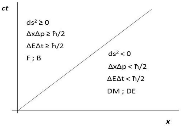
MCA’s results pictured on the space-time diagram. MCA gives the physical meaning to areas where ds² < 0. Such areas create DM and DE. In such areas, so also for DM and DE, reverse HPML and HPET are true. Boundary between those areas and a visible word ds² ≥ 0, of fermions F, bosons B, HPML and HPET is the speed of light in vacuum c

Figure 8

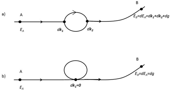
a), when photon reaches the first zero point (black dots), it enters a fermion circulation curve. Through that, it changes its direction dk₁. Thus, at point B, energy of a photon E_B will be equal to the sum of all changes its energy from point A, so its changes of direction and gravitational redshift dg. b) when a photon meets DM circulation, there is no change of direction. Thus, difference between energy at point A and point B will be only through the gravitational redshift E_B = dE_A = dg

9 Conclusions

The sign of direct or indirect confirmed DM detection is still elusive. It means that current DM models do not yield any significant outcomes. Moreover, DE phenomena are also a mystery. This situation generates a need for an alternative explanation.

MCA is a response to this need. It provides a model of DM, through introduction of a third group of particles alongside with fermions and bosons, which interacts only via gravity. Moreover, this idea provides an explanation for most current experimental data on DM and DE on both micro and cosmic scale. Nevertheless, all current MCA predictions need to reach precision. DM mass value and its number in the Universe has to be precisely known, to make any accurate predictions. Assuming that every theory should be calibrated toward experimental data, such a probing of MCA’s DM and DE can back up a theoretical development of this idea. This development should be directed at theory which unifies all interactions. The proof is that MCA provides a new image to similarities between bosonic interaction and gravity. In this new image, the fundamental and only physical quantity is speed of light. Thus, key step in this development is transformation of physical quantities into modifications of a field of the light speed. Laplace transformation should be a natural tool to do it.

Such a theory, since it also includes DM, will have a beautiful practical side. Indeed, by using it, one would be able to make precise predictions on galaxy rotations and literally reshape the visible world around us by changing it into DM. This perspective is based only on MCA’s current stage. New results await with further MCA development. A new results have been mentioned„ because indeed - at this stage of MCA’s development some result could not be seen yet. General reason for that is the fact that MCA was not born to provide a DM candidate or to explain the DE phenomena. The motivation behind MCA creation was the following question - is a quantum particle inertial mass built by more fundamental quantities? This question led to MCA’s particle mass model which surprisingly contains a DM sector. It should be underlined that this model was verified by obtaining m₀ = E/c² from it. This equation is one of the most established equation in the modern physics. In fact, almost every experiment in particle physics proves this equation. Thus, since this proved equation can be obtained from MCA, it can be stated that every proof of m₀ = E/c² also proves MCA, as a model from this equation could be obtained. Taking that into account, the current MCA’s stage and perspective can now be summarized.

Since the established m₀ = E/c² was obtained from MCA’s mass model, using MCA, it is known what has been. Since MCA introduced DM and DE with all the properties which can explain the current experimental data, it is known what is. And since MCA directs further experiments, it could be known what will be. That is a proof that MCA could become a foundation for further theory.

References

[1] Chojnowski M., On Multi-Cohesive Areas, Quant. Matt., 2015, 4(5), 533-547.10.1166/qm.2015.1228Suche in Google Scholar
[2] Chojnowski M., Dark Matter Model from Idea of Multi Cohesive Areas, Canad. J. Phys., 2017, 95(10), 941-949.10.1139/cjp-2017-0144Suche in Google Scholar
[3] Milgrom M., MOND theory, Can. J. Phys., 2015, 93(2), 107-118.10.1139/cjp-2014-0211Suche in Google Scholar
[4] Freese K., Status of Dark Matter in the Universe, Int. J. Mod. Phys. D 26(6), 325-35510.1142/9789813226609_0018Suche in Google Scholar
[5] Roszkowski L., Sessolo E.M., and Trojanowski S., WIMP dark matter candidates and searches - current issues and future prospects, Rept. Prog. Phys. 2018, 81(6), 066201 - 06660110.1088/1361-6633/aab913Suche in Google Scholar PubMed
[6] Barkana R., Possible interaction between baryons and dark-matter particles revealed by the first stars, Nature, 2018, 555, 71-74.10.1038/nature25791Suche in Google Scholar PubMed
[7] Borowiec A., Godłowski W., Szydłowski M., Int. J. Geom. Methods Mod. Phys., 2007, 04 (01), 183-196.10.1142/S0219887807001898Suche in Google Scholar
[8] Ajello M. et al., Phys. Rev. Lett. 116, (2016), (16), 161101.10.1103/PhysRevLett.116.161101Suche in Google Scholar PubMed
[9] Abel C., Ayres N.J., Ban G., Bison G., Bodek K., Bondar V., Daum M., Fairbairn M., Flambaum V.V., Geltenbort P., et al., Search for axionlike dark matter through nuclear spin precession in electric and magnetic fields, Phys. Rev. X, 2017, 7, 041034.10.1103/PhysRevX.7.041034Suche in Google Scholar
[10] Marsh M.C. et al., A new bound on axion-like particles, J. Cosmol. Astropart. Phys., 2017, 036.10.1088/1475-7516/2017/12/036Suche in Google Scholar
[11] Akerib S. et al., Phys. Rev. Lett., 2016, 116(16), 161301.10.1103/PhysRevLett.116.161301Suche in Google Scholar PubMed
[12] Aprile E. et al., Search for WIMP Inelastic Scattering off Xenon Nuclei with XENON100, Phys. Rev. D, 2017, 96, 022008.10.1103/PhysRevD.96.022008Suche in Google Scholar
[13] Einstein A., Zur Elektrodynamik bewegter Körper, Ann. Phys., 1905, 322, 891-921.10.1002/andp.19053221004Suche in Google Scholar
[14] Kuhn T.S., The Structure of Scientific Revolutions, 2009, Polish edition by Wydawnictwo Aletheia, Warszawa.Suche in Google Scholar
[15] Huterer D., Shafer D.L., Dark energy two decades after: observables, probes, consistency tests, Rep. Progr. Phys., 2018, 81(1), 016901.10.1088/1361-6633/aa997eSuche in Google Scholar PubMed
[16] Farnes J.S., A Proposal for a Unifying Theory of Dark Energy and Dark Matter, [arXiv:1712.07962v1].Suche in Google Scholar
[17] Hohmann M., Wohlfarth M.N.R., No-go theorem for bimetric gravity with positive and negative mass, Phys. Rev. D, 2009, 80, 104011.10.1103/PhysRevD.80.104011Suche in Google Scholar
[18] Hohmann M., Wohlfarth M. N. R., Repulsive gravity model for dark energy, Phys. Rev. D, 2010, 81, 104006.10.1103/PhysRevD.81.104006Suche in Google Scholar
[19] Abdallah H. et al., Search for ϒ-ray line signals from dark matter annihilations in the inner Galactic halo from ten years of observations with H.E.S.S, Phys. Rev. Lett., 2018, 120, 201101.10.1103/PhysRevLett.120.201101Suche in Google Scholar PubMed
[20] Lisanti M., Mishra-Sharma S., Rodd N. L.Safdi B. R., A Search for Dark Matter Annihilation in Galaxy Groups, Phys. Rev. Lett, 2018, 120, 101101.10.1103/PhysRevLett.120.101101Suche in Google Scholar PubMed
[21] Macias O., Gordon C., Crocker R. M., Coleman B., Paterson D., Horiuchi S., Pohl M., Galactic bulge preferred over dark matter for the Galactic centre gamma-ray excess, Nat. Astron., 2018, 2, 387-392.10.1038/s41550-018-0414-3Suche in Google Scholar
[22] Iliopoulos J., Introduction to the Standard Model of the Electro-Weak Interactions, CERN Yellow Rep., 2016, 5, [arXiv:1305.6779].Suche in Google Scholar
[23] Perkins D.H., Introduction to high energy physics, 2004, Wydawnictwo Naukowe PWN SA, 4th edition, Warszawa.Suche in Google Scholar
[24] Norwood J., Twentieth Century Physics, 1982, Vol.1, Polish Scientific Publisher, Warszawa.Suche in Google Scholar
[25] Schrödinger, E., Quantisierung als Eigenwertproblem. Ann. Phys., 1926, 384, 361-376.10.1002/andp.19263840404Suche in Google Scholar
[26] Shankar R., Principles of Quantum Mechanics, Polish Version, 2006, Wydawnictwo Naukowe PWN, Warszawa.Suche in Google Scholar
[27] Dawydow A.S., Quantum Mechanics, 1967, Państwowe Wydawnictwo Naukowe, Warszawa.Suche in Google Scholar
[28] Landau L.D., Lifszyc E.M., Course of Theoretical Physics - Quantum mechanics, 1975, Polish version Vol. 2, Polskie Wydawnictwo Naukowe PWN, Warszawa.Suche in Google Scholar
[29] Landau L. D., Lifszyc E. M, Field Theory, Vol 2, Polish version, Państwowe Wydawnictwo Naukowe PWN, Warszawa 1973.Suche in Google Scholar
[30] Schiff L. I., Quantum Mechanics, 1977, Vol. 1, Polish version, Państwowe Wydawnictwo Naukowe, Warszawa.Suche in Google Scholar
[31] Rozemat L. A.,et al, Violation of Heisenberg’s Measurement-Disturbance Relationship by Weak Measurements, Phys. Rev. Lett., 2012, 109, 100404.10.1103/PhysRevLett.109.100404Suche in Google Scholar PubMed
[32] Wróblewski A.K., Zakrzewski J.A., Introduction to Physics, 1984, Państwowe Wydawnictwo Naukowe, Warszawa.Suche in Google Scholar
[33] Landau L. D., Lifszyc E. M„ Course of Theoretical Physics - Mechanics, Electrodynamic, 1975, Vol. 1, Polish version, Polskie Wydawnictwo Naukowe PWN, Warszawa.Suche in Google Scholar
[34] Gaberdiel M. R., An Introduction to conformal field theory, Rept. Prog. Phys., 2000, 63, 607-667.10.1088/0034-4885/63/4/203Suche in Google Scholar
[35] Ginsparg P., Applied Field Theory, 1988, arXiv:hepth/9108028v1.Suche in Google Scholar
[36] Leitner R., Basics of the higher mathematics, Technical - Scientific Publisher, 1995, Vol. 2, Warszawa.Suche in Google Scholar
[37] Kopczyński W., Trautman A., Time-Space and Gravity, 1891, Vol.1, Polish Scientific Publisher, Warszawa.Suche in Google Scholar
[38] Trajdos T., Mathematics for Engineers, 1981, Scientific and Technology Publishers, Warszawa.Suche in Google Scholar
[39] Średniawa B., Hydrodynamic and Elasticity Theory, 1977, Vol. 1, Polish Scientific Publisher, Warszawa.Suche in Google Scholar
[40] Tawfik A.N., Diab A.M., Int. J. Mod. Phys. D, 2014, 23(12), 1430025.10.1142/S0218271814300250Suche in Google Scholar
[41] Carroll S., Explain it in 60 seconds: Bosons. Symmetry Magazine. Fermilab/SLAC. Retrieved 15 February 2013, http://www.symmetrymagazine.org/article/january-2013/bosonsSuche in Google Scholar
[42] Wilczek F., Central Eur. J. Phys, 2012, 10, 1021-1037.10.2478/s11534-012-0121-0Suche in Google Scholar
[43] Das Gupta P., General Relativity for Pedestrians - First 6 lectures, arXiv:1604.00951Suche in Google Scholar
[44] Bierestecki W.B., Lifszyc E.M, Pitajewski L.P., Relativistic Quantum Theory, 1967, Vol. 1, Państwowe Wydawnictwo Naukowe, Warszawa.Suche in Google Scholar
[45] Penrose R., The Road to Reality. A complete Guide to the Laws of the Universe, 2004, Prószyński Media Sp. Z o.o, Warszawa.Suche in Google Scholar
[46] Ni G-J., A new insight into the negative-mass paradox of gravity and the accelerating universe, Rel. Grav. Cosmol., 2004, 1, 123-136.Suche in Google Scholar
[47] Belletête J., Paranjape M. B., On negative mass, Int. J. Mod. Phys. D,2013, 22, 1341017.10.1142/S0218271813410174Suche in Google Scholar
[48] Karaśkiewicz E., Courses of Theory of Vectors and Tensors, 1964, Państwowe Wydawnictwo Naukowe, Warszawa.Suche in Google Scholar
[49] Busch P., The Time-Energy Uncertainty Relation, Time in Quantum Mechanics, eds. J. G. Muga, R. Sala Mayato, I.L. Egusquiza, 2002, Springer-Verlag, Berlin.Suche in Google Scholar
[50] Deffner S., Campbell S., Quantum speed limits: from Heisenberg’s uncertainty principle to optimal quantum control, J. Phys. A: Math. Theor., 2017, 50, 453001.10.1088/1751-8121/aa86c6Suche in Google Scholar
[51] de Cosa A., On behalf of the CMS, ATLAS collaborations, LHC results for dark matter from ATLAS and CMS, arXiv:1510.01516v1.Suche in Google Scholar
[52] Bransden B.H., Evans D., Major J.V., The Fundamental Particles, 1981, Państwowe Wydawnictwo Naukowe, Warszawa.Suche in Google Scholar
[53] Muñoz J.B. et al., A small amount of mini-charged dark matter could cool the baryons in the early Universe, Nature, 2018, 557, 684-686.10.1038/s41586-018-0151-xSuche in Google Scholar PubMed
[54] Grebiszkow K., Physics of hevy ions collisions - lecture 6, 2017/2018, http://www.if.pw.edu.pl/~kperl/HIP/wyklad6.pdfSuche in Google Scholar
[55] Undagoitia T.M., Rauch L., Dark matter direct-detection experiments, J. Phys., 2016, G43(1), 013001.10.1088/0954-3899/43/1/013001Suche in Google Scholar
[56] Pitjev N.P., Pitjeva E.V., Astron. Lett., 2013, 39, 141-149.10.1134/S1063773713020060Suche in Google Scholar
[57] Read J.I., The local dark matter density, J. Phys. G, 2014, 41, 063101.10.1088/0954-3899/41/6/063101Suche in Google Scholar
[58] Salucci P., Nesti F., Gentile G., Frigerio C. M., The dark matter density at the Sun’s location, Astron. Astrophys, 2010, 523, A83.10.22323/1.161.0041Suche in Google Scholar
[59] de Blok W.J.G., The Core-Cusp Problem, Adv. Astron., 2010, 789293.10.1155/2010/789293Suche in Google Scholar
[60] Bernala B.N., Fongc C.S., Fonseca N., Sharing but not caring: dark matter and the baryon asymmetry of the universe, J. Cosmol. Astropart. Phys., 2016, 2016.10.1088/1475-7516/2016/09/005Suche in Google Scholar
[61] Rubinowicz W., Krolikowski W., Theoretical Mechanics, 1998, Państwowe Wydawnictwo Naukowe, Warszawa.Suche in Google Scholar
[62] Almeida J.B., Optical Interpretation of Special Relativity and Quantum Mechanics, arXiv:physics/0010076.Suche in Google Scholar
[63] Elsayed T.A., A Generalization of Fermat’s Principle for Classical and Quantum Systems, Phys. Lett. A, 2014, 378, 3205-3209.10.1016/j.physleta.2014.09.032Suche in Google Scholar
[64] Frolov V.P., Generalized Fermat’s principle and action for light rays in a curved spacetime, Phys. Rev. D, 2013, 88, 064039.10.1103/PhysRevD.88.064039Suche in Google Scholar
[65] Smolin L., What are we missing in our search for quantum gravity?, arXiv:1705.09208v1.Suche in Google Scholar
[66] Szydlowski M., Stachowski A., Borowiec A., Wojnar A., Do sewn up singularities falsify the Palatini cosmology?, Europ. Phys. J. C, 2016, 76(10), 567.10.1140/epjc/s10052-016-4426-9Suche in Google Scholar
[67] Pusey M. F., Barrett J., Rudolph T., On the reality of the quantum state, Nat. Phys., 2012, 8, 475-478.10.1038/nphys2309Suche in Google Scholar
[68] Barbour J., The Nature of Time, arXiv:0903.3489.Suche in Google Scholar
[69] Barbour J., The End of Time: The Next Revolution in Our Understanding of the Universe, 2018, Vol. 1, Copernicus Center Press Sp. z.o.o., Kraków.Suche in Google Scholar
[70] S. Weinberg, Dreams of a Final Theory, 1994, Wydawnictwo Alkazar, Warszawa.10.1119/1.17723Suche in Google Scholar
[71] Corda C., Interferometric detection of gravitational waves: the definitive test for General Relativity, Int. J. Mod. Phys., 2009, D18, 2275-2282.10.1142/S0218271809015904Suche in Google Scholar
© 2019 M. Chojnowski, published by De Gruyter
This work is licensed under the Creative Commons Attribution 4.0 International License.
Artikel in diesem Heft
- Regular Articles
- Non-equilibrium Phase Transitions in 2D Small-World Networks: Competing Dynamics
- Harmonic waves solution in dual-phase-lag magneto-thermoelasticity
- Multiplicative topological indices of honeycomb derived networks
- Zagreb Polynomials and redefined Zagreb indices of nanostar dendrimers
- Solar concentrators manufacture and automation