A new-type intelligent monitoring anchor system for CFRP strand wires based on CFRP self-sensing

Zheng-Nan Jing; Rong-Gui Liu

doi:10.1515/secm-2025-0051

Article Open Access

A new-type intelligent monitoring anchor system for CFRP strand wires based on CFRP self-sensing

Zheng-Nan Jing and Rong-Gui Liu

Published/Copyright: April 12, 2025

Published by

Become an author with De Gruyter Brill

Submit Manuscript Author Information

From the journal Science and Engineering of Composite Materials Volume 32 Issue 1

Abstract

In order to explore the feasibility of the structural health monitoring on the in-service anchor system for carbon fiber-reinforced polymer (CFRP) strand wires, the relative theoretical analysis and experimental tests were conducted. The piezoresistive model for CFRP strand wires was established by theoretical deduction. The damage model of the anchor system at different load stages of the anchorage zone was established by theoretical derivation. Thereby, the regional distribution monitoring methodology of the anchor system was established based on the above two models. The tensile experiments on the anchor system for the CFRP strand wires were carried out, and the typical mechanical and electrical features were ascertained, including volt–ampere characteristics, resistance–strain relationship, strain sensitivity, and the distribution of shear and tensile stresses along the anchorage zone. The results show the theoretical results are in line with the experimental measurements, with a maximum error of below 15%. This indicates excellent applicability and reliability of self-monitoring on the anchoring systems throughout loading.

Keywords: anchor; CFRP strand wire; piezoresistive model; damage model; regional distribution monitoring

1 Introduction

Due to the disadvantages, including the large weight and weak corrosion resistance of steel cables, there are many limitations when they are applied to long-span bridges (Figure 1) [1,2,3]. However, the carbon fiber-reinforced polymer (CFRP) [4,5,6,7,8] has been found to possess outstanding mechanics characteristics when it is used to replace the traditional steel cable, such as high strength-to-weight ratio, strong resistance against corrosion, and excellent fatigue performance.

Figure 1

The cable-stayed bridge with prestressed cables: (a) prestressed cable and (b) anchor system.

The CFRP prestressed cables suffer from repeated actions from traffic loads, the wind load, and other loads in service, which readily damage their anchor systems, resulting in possible fatigue failures [9,10,11]. Therefore, real-time and full-field health monitoring is particularly significant for the anchor system of the CFRP prestressed cables.

Usually, a large number of sensing elements should be embedded into structures to monitor their safety performance when applied to the traditional structural health monitoring (SHM) methods [12,13,14,15]. These treatments may destroy the structure's integrity and, accordingly, weaken its mechanical performance. As for the nondestructive testing methods applied nowadays (Figure 2), some challenges occur when used in the anchor systems due to their complicated operation, heavy workload, and long duration of test [16,17,18].

Figure 2

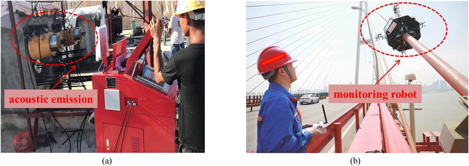
The health monitoring of prestressed cables: (a) acoustic emission detection and (b) monitoring robot.

In contrast, CFRP composites possess some intelligent characteristics. This indicates that it could be used to implement SHM during the whole service lifetime of CFRP strand wire cables. The mechanics and intelligence aspects of the CFRP composite can be utilized to develop an intelligent cable anchoring system to meet the mechanical requirements and simultaneously monitor itself real-time state. Numerous studies have been carried out in this field, as classified into two aspects as follows.

1.1 Failure analysis and design optimization of the CFRP anchor system

Fang and Liang [19] conducted an experimental investigation on a new straight-tapered-straight configuration anchor. The results indicated that the replacement of a straight shape with a tapered shape at the end of the anchor reduced the stress concentration and improved the anchoring efficiency coefficient. Mei et al. [20] divided the tapered configuration anchor into four parts, with different parts filled with varying stiffness bonding media. The results indicated that when the bonding medium stiffnesses were 32, 26, 8, and 4 GPa, respectively, in a sequence of four parts, the anchoring efficiency coefficient reached the highest level of 95.8%. Jing et al. [21] designed an arc-cone new-type configuration anchor to relieve stress concentration in the CFRP strand wire. In this way, they enhanced the anchoring efficiency coefficient to up to 99.7%. Xie et al. [22] conducted cyclic loading tests on tapered configuration anchors. The results showed that the maximum stress level and the stress ratio significantly influenced the fatigue performance of the anchors. Cyclic loading at a relatively high stress level was beneficial to the synergistic action of the anchor assemblies. Xie et al. [23] conducted constant-amplitude fatigue tests on adhesively bonded anchors with different fatigue stress ratios. A fatigue damage prediction model was established based on their experimental results.

From the above research, we found that previous studies mainly focused on the bonding media used in the anchor barrel, the interfacial performance, the fatigue performance, and the corresponding crucial effect factors. The distributions of the tensile and interfacial shear stresses of the CFRP strand wire have not been explored enough yet under different loading stages.

1.2 Intelligent sensing characteristics and engineering applications of the CFRP sensor

Conor and Owston [24] proposed a piezoresistive model using the electric conduction characteristics experiments on a variety of CFRP monofilaments. The results showed that when the sensitivity K ranged from 0.3 to 1.8, the relationship between the external force and resistance was highly linear. Xu [25] conducted a series of experiments to explore the influence of manufacturing technologies (including brushing technology, vacuum technology, and roll-extrusion technology) as well as the carbon powder dosage in the resin matrix on the piezoresistive properties of the CFRP sensors. The results indicated that the brushing technology results in a preferable self-sensing at a carbon powder dosage of 6%. Le [26] carried out experiments to explore the effect of the acidizing modification method (using vitriol or nitric acid) and the nano-carbon dosage in the resin matrix on the piezoresistive effect of the CFRP sensor. The results indicated that the CFRP sensor resistivity was reduced by 30% after acidification; meanwhile, its electrical conductivity was the highest when the carbon nanometer powder dosage was 8–10%. Liu [27] manufactured the CFRP–OFBG sensor (CFRP as the encapsulation material) and applied it in prestressed concrete beam structures. The results showed that when the sensor length was 150 mm, the strain transfer efficiency (i.e., the strain of CFRP to the substrate strain) exceeded 80%. The error between the theoretical and experimental results was within 10%. Yang [28] manufactured the CFRP–FBG sensor (CFRP as the encapsulation material) and applied it in bridge structures to research the regularization index difference of strain influence line for damage location and damage degree based on the damage recognition theory using within a linear range with a long gage. The experimental results indicated that damage monitoring accuracy was related to the bridge stiffness and sensor distribution. The error decreased gradually and is limited in the scope of 5–8% after the optimization of the sensor positions.

The above studies mainly focused on manufacturing technology, electrical conductivity, sensitivity improvement, CFRP-O/FBG encapsulation, and relative application in structures. The piezoresistive effect aiming at CFRP strand wires has not been studied thoroughly. In this context, the piezoresistive model of the CFRP stand wire was established based on the damage model and was applied to deduce the regional distribution monitoring model of the new-type anchor. The corresponding strains and resistance signal of the CFRP stand wire were collected in different zones and damage processes. Finally, the damage degree of the new-type anchor was identified and determined.

2 Theoretical analysis

In this section, the theoretical analysis was carried out, including three aspects: (1) piezoresistive model of the CFRP strand wire, (2) damage model of the new-type anchor from the elastic stage to the failure stage, and (3) regional distribution monitoring model of the new-type anchor system.

2.1 Piezoresistive model of the CFRP strand wire

The total strain energy equation of the CFRP strand wire is derived by combining elastic strain energy theory and the composite material mixing law [29,30]. The total potential energy equation of the CFRP strand wire in a passive electrostatic field is derived by combining the Maxwell velocity distribution law of electrons and the kinematic equation. The relationship between the strain constitutive and electrical conductivity of the CFRP strand wire is established based on Thomson’s theorem and variational principle [13,14,15].

2.1.1 Mechanical analysis

The relationship between the off-axial strain and axial strain of the CFRP strand wire is explored first since the strand wire is different from the bar after loading.

The strand wire meets the following requirements (Figure 3) based on the geometric conditions of CFRP strand wires:

(1) x = r ⋅ sin ( t ) y = r ⋅ cos ( t ) z = k ⋅ t ,

where t is the helical angle, r is the helical radius, and k is the helical parameter.

Figure 3

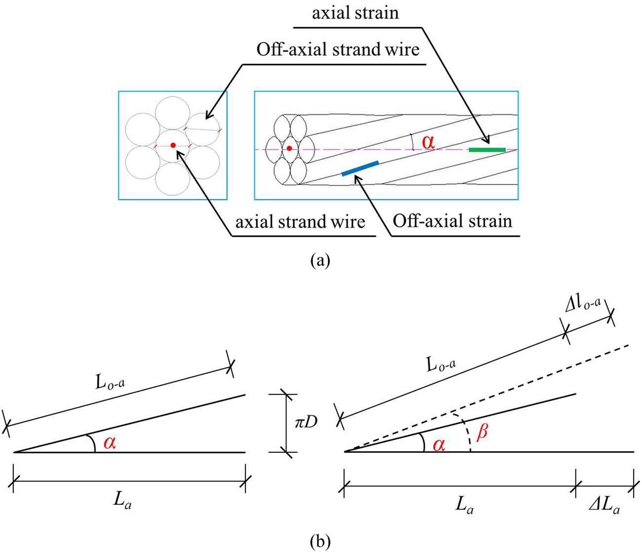
The relation between axial strain and off-axial strain of the CFRP strand wire: (a) section of the CFRP strand wire and (b) relation between axial strain and off-axial strain of the CFRP strand wire before and after loading.

Since the strain gauge is attached to the outside of the strand wire,

(2) r = d a 2 + d o − a k = S 2 π ,

where d a , d o − a are the diameters of the axial and off-axial strand wire, respectively, and S is the lay length.

By integrating t along the longitudinal direction, the helical length per unit lay length can be obtained as follows:

(3) L o − a = ∫ 0 2 π r 2 sin 2 ( t ) + r 2 cos 2 ( t ) + L a 2 π d t = ( 2 π r ) 2 + L a 2 tan ( α ) = π ( d a + 2 d o − a ) L a ; tan ( β ) = π ( d a 1 + 2 d o − a 1 ) L a + Δ L a ,

where L o − a , L a are the helical and axial lengths, α , β are the off-axial angles before and after deformation, and Δ L a are the axial lengths.

The deformation is

(4) Δ L a = L a 1 − L a , Δ d a = d a 1 − d a Δ L o − a = L o − a 1 − L o − a , Δ d o − a = d o − a 1 − d o − a ⇒ Δ L o − a = Δ L a ⋅ cos ( β ) ,

where Δ L a , Δ L o − a are the change lengths of the axial and off-axial strand wire and Δ L a 1 , Δ L o − a 1 are the lengths after the change of axial and off-axial strand wires.

The engineering practice shows that the axial strain of the CFRP strand wire changes from 0 to 9.5 × 10⁻³ after loading, and the variation in the angle between the axial and off-axial wire ranges from 2 to 3% [2]. Therefore, the angle α can be approximately equal to β . The relation between the axial strain and off-axial strain of the CFRP strand wire before and after loading is

(5) ε a = Δ L a L a = L a 1 − L a L a ε o − a = Δ L o − a L o − a = L o − a 1 − L o − a L o − a ⇒ ε o = ε o − a ⋅ 1 cos ( α ) ⋅ cos ( β ) ⇒ ε o ≈ ε o − a ⋅ 1 cos ( α ) 2 ,

where ε a , ε o − a are the axial and off-axial strains of the strand wire, and α , β are the included angles between the axial and off-axial strand wire.

By combining the elastic strain energy theory and composite material mixing law, the strain energy density function equation of the CFRP strand wire is derived as follows:

(6) u c ( ε i j ) = ∫ 0 ε i j σ i j ⋅ d ε i j = 1 2 σ i j ⋅ ε i j ,

where i , j = 1 , 2 , 3 , σ i j is the stress tensor; ε i j is the strain tensor; and u c ( ε i j ) is the strain energy density function of the CFRP.

From the above formula,

(7) u c ( ε i j ) = 1 2 ( σ x ε x + σ y ε y + σ z ε z + τ x y γ x y + τ x z γ x z + τ y z γ y z ) ,

where σ , ε are the normal stress and normal strain, respectively; τ , γ are shear stress and shear strain, respectively; and x , y , z represent the three axials in all directions.

According to Hooke’s law, the following formulae can be obtained:

(8) σ x = E 1 − μ 2 ( ε x + μ ε y ) σ y = E 1 − μ 2 ( ε x + μ ε x ) τ x y = E 2 ( 1 + μ ) γ x y ,

where E is the elasticity modulus of the CFRP strand wire and μ is the Poisson’s ratio.

Based on the composite material mixing law, the following formula is obtained:

(9) E = E cfrp V cfrp + E epoxy V epoxy ,

where E cfrp , E epoxy are the elasticity modulus of CFRP and epoxy resin, respectively, and V cfrp , V epoxy are the volume fraction of the CFRP fiber and epoxy resin, respectively.

The elastic strain energy density of the CFRP strand wire is expressed as follows:

(10) u c ( ε i j ) = E 2 ( 1 − μ 2 ) ( ε x 2 + ε y 2 + 2 μ ⋅ ε x ε y ) + E 4 ( 1 + μ ) ⋅ γ x y 2 .

At this time, the total strain energy of the CFRP strand wire is

(11) U M , c = ∭ V u c ( ε i j ) d V = E 2 ( 1 + μ ) ∭ V μ 1 − μ ( ε x + ε y ) 2 + 1 1 − μ ( ε x 2 + ε y 2 ) + 1 2 γ x y 2 d V ,

where U M , c is the total strain energy density function of the CFRP strand wire.

2.1.2 Electrical analysis

By combining the Maxwell velocity distribution law of electrons and the kinematic equation, the total potential energy equation of the CFRP strand wire in a passive electrostatic field is derived:

(12) U E , c = 1 2 ∭ V ρ q ⋅ φ d V ,

where ρ q is the density of the volume charge, φ is the electric potential, and U E , c is the total potential energy function.

According to the Maxwell distribution equation, the electrical conductivity of the CFRP strand wire is as follows:

(13) C = n e ⋅ q e 2 m e t e = n e ⋅ q e 2 m e ⋅ λ e v e ,

where n e , m e are the electronic quantity and quality, respectively; q e is the quantity of the electric charge; t e is the average time between electron collisions; λ e is the free path distance of the electron movement; v e is the average rate of the electron migration; and C is the electrical conductivity.

Consider the influence of the temperature effect in service environments. Therefore, the electrical characteristics of CFRP sensors are related to the Fermi level density based on the quantum theory of conductivity and heat conduction. Namely, the equation is

(14) v F , e = 2 ε F m e ,

where v F , e is the Fermi velocity and ε F is the Fermi energy.

Then, Equation (13) is rewritten as

(15) C = n e q e 2 λ e ′ ⋅ 1 / 2 m e ⋅ ε F ,

where λ e ′ is the corresponding free path distance of the electron movement of electron wave scattering.

Furthermore, the bulk charge density is

(16) ρ q = n e ⋅ q e = C ⋅ 2 m e ε F q e λ e ′ ,

yielding the total potential energy of the CFRP sensor as

(17) U E , c = ∭ V φ ⋅ C ⋅ 2 m e ε F q e λ e ′ d V .

2.1.3 Resistance–strain relationship

By combining the potential energy function of the CFRP sensor from the mechanical and electrical aspects above, the total potential energy of the CFRP sensor in the passive electrostatic field can be obtained as follows:

(18) U T , c = U M , c + U E , c = E 2 ( 1 + μ ) ∭ V μ 1 − μ ( ε x + ε y ) 2 + 1 1 − μ ( ε x 2 + ε y 2 ) + 1 2 γ x y 2 d V + ∭ V φ ⋅ C ⋅ 2 m e ε F q e λ e ′ d V .

The total potential energy follows Thomson’s law in the passive electrostatic field. Therefore, the governing equation of conductivity C and strain ε of the CFRP sensor can be obtained based on the variational principle (let δ U T , c = 0 in Equation (18)):

(19) C = − ξ + 1 4 η ⋅ C 1 ε x 2 − ξ η ⋅ C 1 ε x ε y − ξ + 1 4 η ⋅ C 1 ε y 2 − 1 2 η ⋅ C 1 γ x y 2 + C 0 C 1 = E 2 ( 1 + μ ) , ξ = 2 μ 1 − μ , η = φ 2 m e ε F q e λ e ′ ,

where C 1 , C 0 , ξ and η are constants.

According to Ohm’s law, the resistance R , resistivity ρ , and conductivity C of the CFRP sensor meet the following requirements:

(20) R = ρ ⋅ L A = 1 C ⋅ L A ,

where L and A are the length and the cross-sectional area, respectively.

Considering that axial tensile failures often occur in the anchor zone, the shear strain γ x y can be ignored, whereas the Poisson effect μ = ε y / ε x should be considered in Equation (19). Incorporating Equations (19) into (20) yields the following relationship between the resistance R and the strain ε x :

(21) R = 1 a ε x 2 + b ⋅ L A ,

where a , b are the material parameters.

According to the principle of elasticity [29],

(22) ε x = L − L 0 L 0 = Δ L L 0 ⇒ L = ( 1 + ε x ) L 0 ,

where L 0 , Δ L are the initial length and variation of length, respectively.

The combination of Equations (21) and (22) yields the following equation:

(23) R = 1 + ε x a ε x 2 + b ⋅ L 0 A .

The sensitivity K denotes the resistance change rate Δ R / R 0 per unit strain ε x in a CFRP sensor. Namely:

(24) R − R 0 / R 0 ε x = Δ R / R 0 ε x = K Δ R / R 0 = ( a 0 + b i ) ⋅ ε x + a 0 − a i a ⋅ ε x 2 + b ,

where R 0 , Δ R are the initial resistance and variation of resistance, respectively; and a 0 , a i , and b 0 are all unknown constants.

The above model provides theoretical support for analyzing the intelligent sensing performance of the CFRP strand wire.

2.2 Damage model of the new-type anchor

A previous study has shown that the stress distribution in the anchorage zone and interface damage state were important effect factors of anchoring performance. In this section, the local bond-slip constitutive model based on the fracture mechanics theory is used to derive the calculation models of stress distribution in the anchorage zone, CFRP slippage, and ultimate bearing capacity in different loading stages [30].

2.2.1 Fundamental assumptions

The designed new-type arc-cone anchor system [21] is shown in Figure 4.

Figure 4

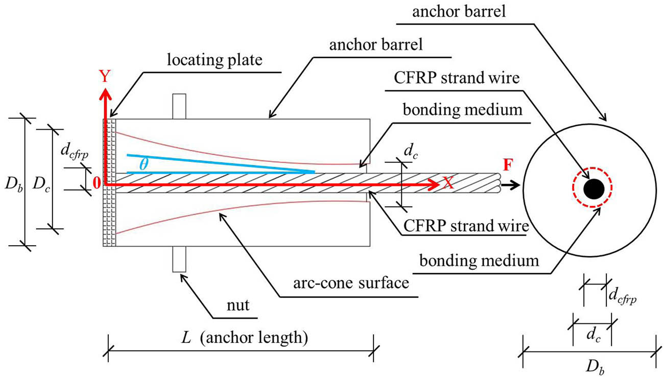
Design parameters of new-type anchors for the CFRP strand wire.

According to the stress state abovementioned, the stress distribution and damage development model of the interface between the CFRP strand wire and the bonding medium were derived in different loading stages. The assumptions are as follows: ① the CFRP strand wire, bonding medium, and anchor barrel are uniform and linearly elastic; ② the stress distribution in the cross-sections of the CFRP stand wire, bonding medium, and anchor barrel are uniform; ③ there is no relative displacement or initial stress at the interface between the CFRP strand wire and bonding medium; and ④ the transverse shear deformations of the CFRP strand wire and bonding medium are ignored.

For simplicity, the anchoring system is divided into two parts: (1) the anchor barrel and bonding medium as the first part (equivalent body) and (2) the CFRP strand wire as the other part.

2.2.2 Governing equations

The simplified model for the mechanical analysis of the new-type anchor is shown in Figure 5.

Figure 5

The simplified micrograph of the new-type anchor for the CFRP strand wire.

Based on the static equilibrium conditions, we can obtain

(25) π 4 d cfrp 2 ⋅ d σ ( x ) = π d c f r p ⋅ d x ⋅ τ ( x ) ⇒ d σ ( x ) d x − 4 τ ( x ) d cfrp = 0 F e = F cfrp ⇒ σ e A e + σ cfrp A cfrp = 0 ,

where d cfrp is the diameter of the CFRP strand wire; σ ( x ) , τ ( x ) are the normal and shear stresses of the CFRP strand wire, respectively; F e , F cfrp are the external forces applied to the equivalent body and CFRP strand wire, respectively; σ e , σ cfrp are normal stress of equivalent body and CFRP strand wire, respectively; and A e , A cfrp are the cross-sectional area of the equivalent body and CFRP strand wire, respectively.

Based on the theory of elastic mechanics [30], the constitutive equation can be written as

(26) τ ( x ) = f ( δ ) σ cfrp = E d u ( x ) cfrp d x σ e = E e d u ( x ) e d x ,

where f ( δ ) is the relative displacement function between the CFRP strand wire and equivalent body, u ( x ) cfrp is the displacement of the CFRP strand wire, u ( x ) e is the displacement of the equivalent body, and E e is the elasticity modulus of the equivalent body.

The slip at the interface between the CFRP strand wire and the bonding medium is

(27) δ ( x ) = u ( x ) cfrp − u ( x ) e .

Substituting Equations (26) and (27) into Equation (25), we obtain:

(28) d 2 δ ( x ) d x 2 − 8 G f τ f 2 ⋅ ψ 2 ⋅ f ( δ ) = 0 σ ( x ) cfrp = τ f 2 2 G f d cfrp ψ 2 ⋅ d δ ( x ) d x ,

where

(29) ψ 2 = τ f 2 2 G f 1 E d cfrp + A cfrp A e E e d cfrp δ ( x ) = f ( δ ) ⇒ G f = ∫ f ( δ ) ⋅ d δ ,

where G f is the fracture energy, τ f is the local bond strength, and δ ( x ) is the relative displacement function.

Equation (28) represents the stress distribution in the anchorage zone (Figure 6). The general solution of the governing equation can be determined once the bond-slip constitutive model is known.

Figure 6

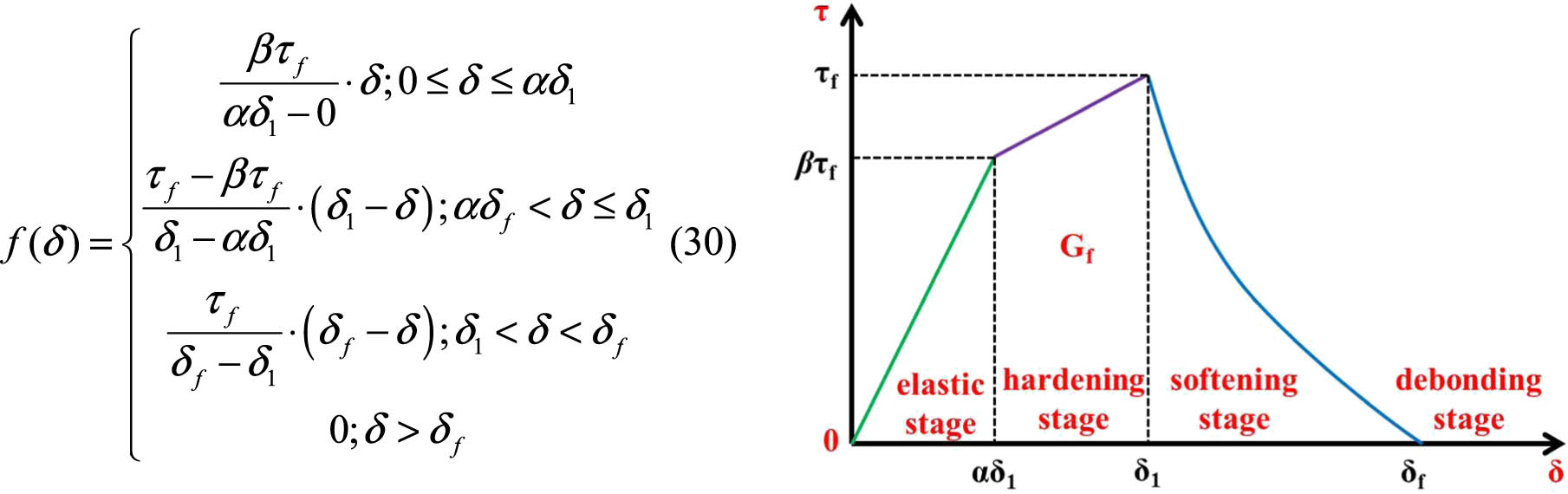
The bond-slip constitutive model of the new-type anchor for the CFRP strand wire.

2.2.3 Bond-slip relationship

Based on previous research [22], a tri-linear hardening bond-slip constitutive model is chosen in this study, as shown in Figure 6:

(30) f ( δ ) = β τ f α δ 1 − 0 ⋅ δ ; 0 ≤ δ ≤ α δ 1 τ f − β τ f δ 1 − α δ 1 ⋅ ( δ 1 − δ ) ; α δ f < δ ≤ δ 1 τ f δ f − δ 1 ⋅ ( δ f − δ ) ; δ 1 < δ < δ f 0 ; δ > δ f ,

where α , β are constants.

2.2.4 Whole damage process analysis

According to the proposed bond-slip model in Section 2.2.3, the governing equation (Equation (28)) can be solved to determine the shear/tensile stress distribution and load–displacement relationship along the interface of the new-type anchor in different stages. The states of elastic, hardening, softening, and debonding are shown in Figure 7.

Figure 7

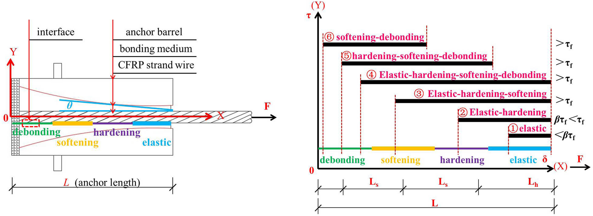
The damage process development of the new-type anchor for the CFRP strand wire.

2.2.4.1 Elastic stage

When the entire anchor zone is elastic, we have x = L ⇒ τ ( x ) < β τ f . Then, Equation (30) for 0 ≤ δ ≤ α δ 1 is applied to Equation (28), yielding

(31) d 2 δ d x 2 − ψ 1 2 δ = 0 ; ( 0 ≤ δ ≤ α δ 1 ) .

The boundary conditions:

(32) x = L , σ cfrp = F A cfrp ; ( tensile-end ) x = 0 , σ cfrp = 0 ; ( free-end ) ,

where

(33) ψ 1 2 = 8 β G f α τ f δ 1 ⋅ ψ 2 = 4 β τ f α δ 1 1 E d cfrp + A 1 A e E e d cfrp .

The displacement, shear stress of interface, and normal stress of the CFRP strand wire are obtained as follows:

(34) δ = α δ cfrp β τ f . F ⋅ d cfro ψ 1 4 A cfrp sinh ( ψ 1 L ) cosh ( ψ 1 x ) τ = F ⋅ d cfrp ψ 1 4 A cfrp sinh ( ψ 1 L ) cosh ( ψ 1 x ) σ cfrp = F A cfrp sinh ( ψ 1 L ) sinh ( ψ 1 x ) ⇒ F = β α . 4 τ f A cfrp d cfrp ψ 1 . Δ δ 1 tanh ( ψ 1 L ) ,

where F is the external force of the anchor; Δ is the displacement of the tensile end (namely, δ = Δ at x = L ); and ψ , h are the material parameters.

2.2.4.2 Elastic-hardening stage

When the load is in the elastic-hardening stage ( x = L ⇒ β τ f < τ ( x ) < τ f ), the interface hardened (hardening zone length L h ). Then, the function ( 0 ≤ δ ≤ α δ 1 , α δ 1 ≤ δ ≤ δ 1 ) of Equation (30) is substituted into the governing Equation (28) to obtain

(35) d 2 δ d x 2 − ψ 1 2 δ = 0 ; ( 0 ≤ δ ≤ α δ 1 ) d 2 δ d x 2 − ψ 2 2 δ = β − α 1 − α δ 1 ψ 2 2 ; ( α δ 1 < δ ≤ δ 1 ) .

The boundary conditions

(36) x = L , σ cfrp = F A cfrp ; x = 0 , σ cfrp = 0 x = L − L h , σ cfrp [ C ( E ) ] ; x = L − L h , δ = α δ 1 ,

where

(37) ψ 2 2 = 8 G f τ f 2 ψ 2 1 − β 1 − α . τ f δ 1 = 1 − β 1 − α . 4 τ f δ 1 1 E cfrp d cfrp + 1 A e E e d cfrp .

The conditions should be divided into two aspects:

① In the elastic zone ( 0 ≤ δ ≤ α δ 1 , 0 ≤ x ≤ L − L h ) ,

(38) δ = α δ 1 cos ( ψ 1 x ) cosh [ ψ 1 ( L − L h ) ] τ = β τ f cos ( ψ 1 x ) cosh [ ψ 1 ( L − L h ) ] σ cfrp = 4 β τ f d cfrp ψ 1 sin ( ψ 1 x ) cosh [ ψ 1 ( L − L h ) ] .

② In the hardening zone ( α δ 1 ≤ δ ≤ δ 1 , L − L h ≤ x ≤ L ) ,

(39) δ = 1 − α 1 − β β δ 1 cosh [ λ 2 ( L − L h − x ) ] − α δ 1 ψ 1 ψ 2 tanh [ ψ 1 ( L − L h ) ] sin [ ψ 2 ( L − L h − x ) ] τ = β τ f cosh [ ψ 2 ( L − L h − x ) ] − 1 − β 1 − α . α τ f ψ 1 ψ 2 tanh [ ψ 1 ( L − h ) ] sin [ ψ 2 ( L − L h − x ) ] σ cfrp = − 4 β τ f d cfrp ψ 2 sinh [ ψ 2 ( L − L h − x ) ] + 4 τ f β ψ 1 d cfrp tanh [ ψ 1 ( L − L h ) ] cos [ ψ 2 ( L − L h − x ) ] .

When the boundary condition (Equation (36)) is substituted into Equation (38), the following equation is obtained:

(40) F = 4 A cfrp β τ f d cfrp ψ 2 sinh ( ψ 1 h ) + 4 τ f β d c f r p ψ 1 tanh [ ψ 1 ( L − L h ) ] cosh ( ψ 1 L h ) Δ = ( 1 − α ) β δ 1 1 − β cosh ( ψ 2 L h ) + α δ 1 ψ 1 ψ 2 tanh [ ψ 1 ( L − L h ) ] sin ( ψ 2 L h ) − β − α 1 − β δ 1 .

2.2.4.3 Elastic-hardening–softening stage

When loads are in the elastic-hardening–softening stage ( x = L ⇒ δ = δ 1 , τ ( x ) > τ f ), the interface softens (hardening zone length L h and softening zone length L s ). The function ( 0 ≤ δ ≤ α δ 1 , α δ 1 ≤ δ ≤ δ 1 , δ 1 ≤ δ ≤ δ f ) of Equation (30) is substituted into the governing Equation (28):

(41) d 2 δ d x 2 − ψ 1 2 δ = 0 ; ( 0 ≤ δ ≤ α δ 1 ) d 2 δ d x 2 − ψ 2 2 δ = β − α 1 − α δ 1 ψ 2 2 ; ( α δ 1 < δ ≤ δ 1 ) d 2 δ d x 2 + λ 3 2 δ = δ f ψ 3 2 ; ( δ 1 < δ ≤ δ f ) .

The boundary conditions are as follows:

(42) x = L , σ cfrp = F cfrp A cfrp ; x = 0 , σ cfrp = 0 x = L − L s , σ cfrp [ C ( E ) ] ; x = L − L s , δ = δ 1 x = L − L h − L s , σ cfrp [ C ( E ) ] ; x = L − L h − L s , δ = α δ 1 ,

where

(43) ψ 3 2 = 8 G f τ f ⋅ 1 δ f − δ 1 . ψ 2 .

At this time, the conditions should be divided into three aspects:

① In the elastic region ( 0 ≤ δ ≤ α δ 1 ) ,

(44) δ = α δ 1 cosh ( ψ 1 x ) cosh [ ψ 1 ( L − L h − L s ) ] τ = β τ f cosh ( ψ 1 x ) cosh [ ψ 1 ( L − L h − L s ) ] σ cfrp = 4 β τ f d cfrp ψ 1 sinh ( ψ 1 x ) cosh [ ψ 1 ( L − L h − L h ) ] .

② In the hardening zone ( α δ 1 ≤ δ ≤ δ 1 ) ,

(45) δ = − ( 1 − α ) δ 1 1 − β . sinh [ ψ 2 ( L − L h − L s − x ) ] sinh ( ψ 2 L h ) + δ 1 ( 1 − α ) β sinh [ ψ 2 ( L − L s − x ) ] ( 1 − β ) sinh ( ψ 2 L h ) − β − α 1 − β δ 1 τ = − τ f sinh [ ψ 2 ( L − L h − L s − x ) ] sinh ( ψ 2 h ) + β τ f sinh [ ψ 2 ( L − L s − x ) ] sinh ( ψ 2 h ) σ cfrp = 4 τ f d cfrp ψ 2 cosh [ ψ 2 ( L − L h − L s − x ) ] sinh ( ψ 2 h ) − β cosh [ ψ 2 ( L − L s − x ) ] sinh ( ψ 2 h ) .

③ In the softening region ( δ 1 ≤ δ ≤ δ f ) ,

(46) δ = − ( 1 − α ) ψ 2 δ 1 1 − β ψ 3 . sin [ ψ 3 ( L − L s − x ) ] [ cosh ( ψ 2 h ) − β ] sinh ( ψ 2 h ) − ( δ f − δ 1 ) cos [ ψ 3 ( L − L s − x ) ] τ = ( 1 − α ) ψ 2 δ 1 τ f ( 1 − β ) ψ 3 ( δ f − δ 1 ) . sin [ ψ 3 ( L − L s − x ) ] [ cosh ( ψ 2 h ) − β ] sinh ( ψ 2 h ) + τ f cos [ ψ 4 ( L − L s − x ) ] σ cfrp = 4 τ f d cfrp ψ 2 . cos [ ψ 3 ( L − L s − x ) ] [ cosh ( ψ 2 h ) − β ] sinh ( ψ 2 h ) − 4 τ f sin [ ψ 3 ( L − L s − x ) ] d c f r p ψ 3 .

When the boundary condition (Equation (43)) is substituted into Equation (46), the following equation is obtained:

(47) F = 4 A cfrp τ f d cfrp ψ 2 . [ cosh ( ψ 2 h ) − β ] cos ( ψ 3 a ) sinh ( ψ 2 h ) + 4 τ f sin ( ψ 3 a ) d cfrp ψ 3 Δ = ( 1 − α ) ψ 2 δ 1 ( 1 − β ) ψ 3 . [ cosh ( ψ 2 h ) − β ] sin ( ψ 3 a ) sinh ( ψ 2 h ) − ( δ f − δ 1 ) cos ( ψ 3 a ) + δ f .

2.2.4.4 Elastic-hardening–softening–debonding stage

When loads are in the elastic-hardening–softening–debonding stage, the debonding zone (crack growth zone) gradually expands along the interface between the CFRP strand wire and equivalent body from the tensile end to the free end (hardening zone length L h , softening zone length L s , and debonding zone length L d ). Then, L in Equations (44)–(47) is substituted with L − L d , and the stress distribution is as follows:

① In the elastic region ( 0 ≤ δ ≤ α δ 1 ) ,

(48) δ = α δ 1 cosh ( ψ 1 x ) cosh [ ψ 1 ( L − L h − L s − L d ) ] τ = β τ f cosh ( ψ 1 x ) cosh [ ψ 1 ( L − L h − L s − L d ) ] σ cfrp = 4 β τ f d cfrp ψ 1 sinh ( ψ 1 x ) cosh [ ψ 1 ( L − L h − L s − L d ) ] .

② In the hardening region ( α δ 1 ≤ δ ≤ δ 1 ) ,

(49) δ = − ( 1 − α ) δ 1 1 − β . sinh [ ψ 2 ( L − L h − L s − L d − x ) ] sinh ( ψ 2 h ) + δ 1 ( 1 − α ) β sinh [ λ 2 ( L − L s − L d − x ) ] ( 1 − β ) sinh ( ψ 2 h ) − β − α 1 − β δ 1 τ = − τ f sinh [ ψ 2 ( L − L h − L s − L d − x ) ] sinh ( ψ 2 h ) + β τ f sinh [ ψ 2 ( L − L s − L d − x ) ] sinh ( ψ 2 h ) σ cfrp = 4 τ f d cfrp ψ 2 cosh [ ψ 2 ( L − L h − L s − L d − x ) ] sinh ( ψ 2 h ) − β cosh [ ψ 2 ( L − L s − L d − x ) ] sinh ( ψ 2 h ) .

③ In the softening region ( δ 1 ≤ δ ≤ δ f ) ,

(50) δ = − ( 1 − α ) ψ 2 δ 1 1 − β ψ 3 . sin [ ψ 3 ( L − L s − L d − x ) ] [ cosh ( ψ 2 h ) − β ] sinh ( ψ 2 h ) − ( δ f − δ 1 ) cos [ ψ 3 ( L − L s − L d − x ) ] + δ f τ = ( 1 − α ) ψ 2 δ 1 τ f ( 1 − β ) ψ 3 ( δ f − δ 1 ) . sin [ ψ 3 ( L − L s − L d − x ) ] [ cosh ( ψ 2 h ) − β ] sinh ( ψ 2 h ) + τ f cos [ ψ 3 ( L − L s − L d − x ) ] σ cfrp = 4 τ f d cfrp ψ 2 . cos [ ψ 3 ( L − L s − L d − x ) ] [ cosh ( ψ 2 h ) − β ] sinh ( λ 2 h ) − 4 τ f sin [ ψ 3 ( L − L s − L d − x ) ] d c f r p ψ 3 .

When the slip-off δ > δ f on the tensile end, the relationship between the displacement and loading is as follows:

(51) P = 4 A cfrp τ f d cfrp ψ 2 . [ cosh ( ψ 2 h ) − β ] cos ( ψ 3 L d ) sinh ( ψ 2 h ) + 4 τ f sin ( ψ 3 L d ) d cfrp ψ 3 Δ = δ f + F A cfrp E cfrp + F A e E e d cfrp = δ f + F ψ 2 d cfrp 2 τ f A cfrp ( β δ 1 − α δ 1 + δ f ) .

2.2.4.5 Hardening–softening–debonding stage

When loads are in the hardening–softening–debonding stage ( x = 0 ⇒ δ = α δ 1 , τ ( x ) > τ f ), the interface hardened-softened and debonded (hardening zone length L h , softening zone length L s , and debonding zone length L d ). The function ( α δ 1 ≤ δ ≤ δ 1 , δ 1 ≤ δ ≤ δ f ) of Equation (30) is substituted into governing Equation (28):

(52) d 2 δ d x 2 − ψ 2 2 δ = β − α 1 − α δ 1 ψ 2 2 ; ( α δ 1 < δ ≤ δ 1 ) d 2 δ d x 2 + λ 3 2 δ = δ f ψ 3 2 ; ( δ 1 < δ ≤ δ f ) .

The boundary conditions are as follows:

(53) x = L h + L s = L − L d , σ cfrp = F cfrp A cfrp ; x = 0 , σ cfrp = 0 x = L h = L − L s − L d , δ = δ 1 x = L h + L a = L − L d , δ = δ f x = L h = L − L s − L d , σ cfrp [ C ( E ) ] .

At this time, the conditions should be divided into two aspects:

① In the hardening region ( α δ 1 ≤ δ ≤ δ 1 ) ,

(54) δ = ( 1 − α ) δ 1 1 − β . cosh ( ψ 2 x ) cosh ( ψ 2 h ) − β − α 1 − β δ 1 τ = τ f cosh ( ψ 2 x ) cosh ( ψ 2 h ) σ cfrp = 4 τ f d cfrp ψ 2 . sinh ( ψ 2 x ) cosh ( ψ 2 h ) .

② In the softening region ( δ 1 ≤ δ ≤ δ f ) ,

(55) δ = δ f − δ f − δ 1 sin ( ψ 3 L s ) sin [ ψ 3 ( L h + L s − x ) ] τ = τ f sin ( ψ 3 L s ) sin [ ψ 3 ( L h + L s − x ) ] σ cfrp = 4 τ f d cfrp ψ 3 . cos [ ψ 3 ( L h + L s − x ) ] sin ( ψ 3 L s ) .

When Equation (55) is substituted into Equation (54), the following formula is obtained:

(56) F = 4 τ f A cfrp d cfrp ψ 3 sin ( ψ 3 L s ) Δ = δ f + F A cfrp E cfrp + F A e E e d cfrp = δ f + F ψ 2 d cfrp 2 τ f A cfrp ( β δ 1 − α δ 1 + δ f ) .

2.2.4.6 The softening–debonding stage

When loads are in the softening–slip stage ( x = 0 ⇒ δ = δ 1 , τ ( x ) > τ f ), the interface has softening–debonding (hardening zone length L h , softening zone length L s , and debonding zone length L d ). The function ( δ 1 ≤ δ ≤ δ f ) of Equation (30) should be substituted into governing Equation (28):

(57) d 2 δ d x 2 + ψ 3 2 δ = δ f ψ 3 2 ; ( δ 1 ≤ δ ≤ δ f ) .

The boundary conditions are as follows:

(58) x = L s = L − L s , σ cfrp = F cfrp A cfrp ; x = 0 , σ cfrp = 0 x = L s = L − L s , δ = δ f .

Then, one obtains the following solution:

(59) δ = δ f − F d cfrp ( δ f − δ 1 ) ψ 3 4 A cfrp τ f . cos ( ψ 3 x ) sin ( ψ 3 L s ) τ = F d cfrp ψ 3 4 A cfrp . cos ( ψ 3 x ) sin ( ψ L s ) σ cfrp = F A cfrp . sin ( ψ 3 x ) sin ( ψ 3 L s ) .

When Equation (58) is substituted into Equation (59), the following formula is obtained:

(60) F = 4 τ f A cfrp d cfrp Δ = δ f + F A cfrp E cfro + F A e E e d cfrp = δ f + F A cfrp E cfrp + F A e E e ( L − L c ) .

2.3 Regional distribution monitoring model of the new-type anchor

Based on the distributed sensing monitoring concept [18], the corresponding resistance signal of the CFRP stand wire (Section 2.1) is measured in different zones, which are divided according to the damage distribution across the anchor zone before the occurrence of failure (Section 2.2). Then, the damage degree of the anchor can be ascertained based on the measured electrical resistance. The distributed sensing monitoring process [18] is shown in Figure 8.

Figure 8

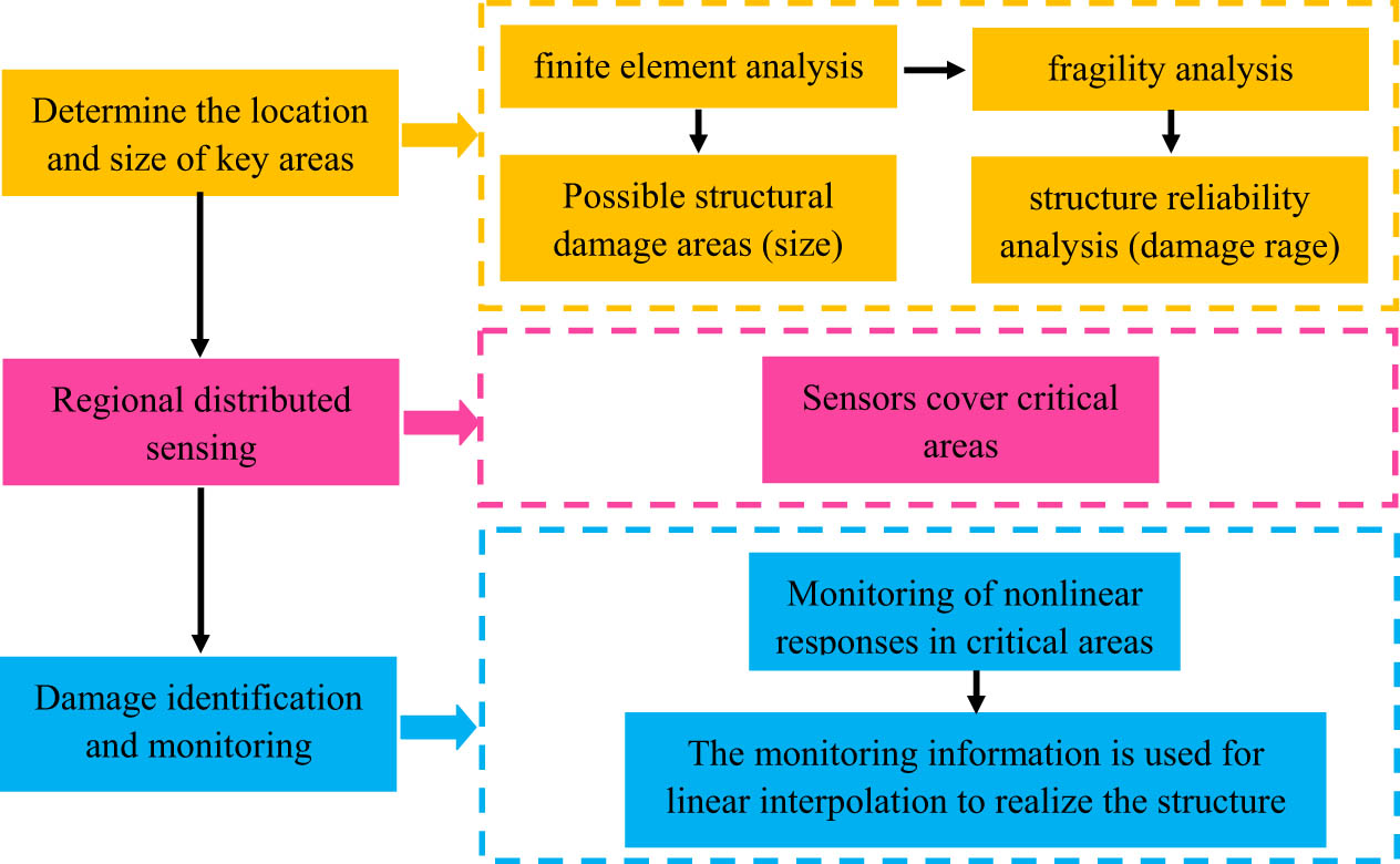
The structure area-distributed sensing monitoring process.

2.3.1 Structural state parameter analysis

Based on the damage analysis of the anchor in Section 2.2, the stress distribution of the anchor is simulated using a finite element method. The physical parameters and parameters [21] in the finite element model are summarized in Tables 1–3. The SolidWorks software [31] is used to establish the assembly model of the anchor for the CFRP strand wire (Figure 9a). Meanwhile, this model is imported into ANSYS Workbench software [32] to generate the finite element model (Figure 9b). The numerical results are shown in Figure 9c and d.

Table 1

Design parameters of the new-type anchor for the CFRP strand wire

Anchor length L (mm)	d _cfrp (mm)	D _b(mm)	D _c (mm)	d _c(mm)	Cone radius (mm)
300	15.2	60	50	25	4,800

Table 2

Parameters of all materials

Component	Material	Elasticity modulus (GPa)	Poisson’s ratio	Element type	Material behavior
Anchor barrel	Cr40	211	0.33	Solid 186	Bilinear elastoplasticity
Bonding medium	UHPC	35	0.19	Solid 187	Bilinear elastoplasticity
CFRP strand wire	—	155 (axial)/10 (radial)	0.27/0.02	Solid 186	Linear elasticity

Table 3

Settings of the interface contact

Interface	Type	Interfacial friction coefficient	Formula	Contact element
Primary interface	Frictional	0.5	Augmented Lagrange	Contact pairs
Second interface	Bonded	—	MPC	Conta 174
CFRP strand wire	Bonded	—	MPC	Targe 170

Figure 9

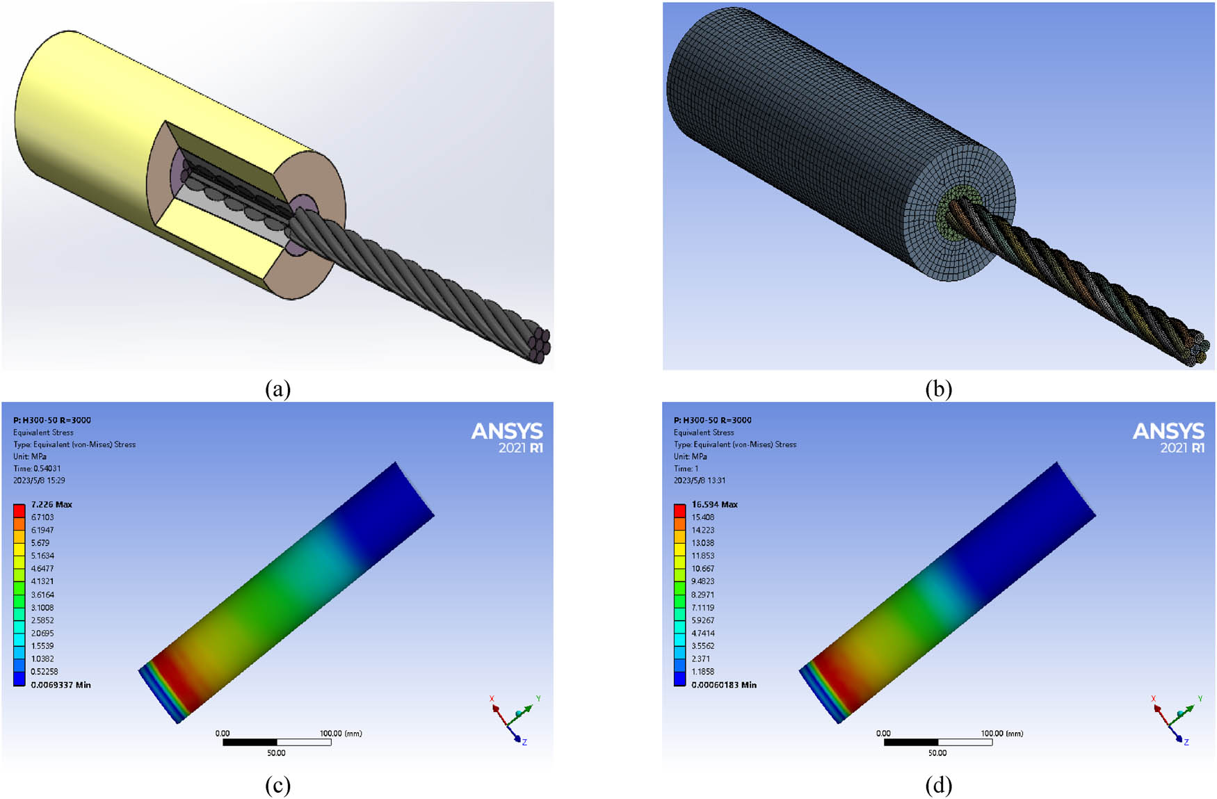
The stress distribution of the new-type anchor system for the CFRP strand wire: (a) physical model of the new-type anchor system; (b) finite element model of the new-type anchor system; (c) stress distribution of the new-type anchor system under 150 MPa; and (d) stress distribution of the new-type anchor system under 300 MPa.

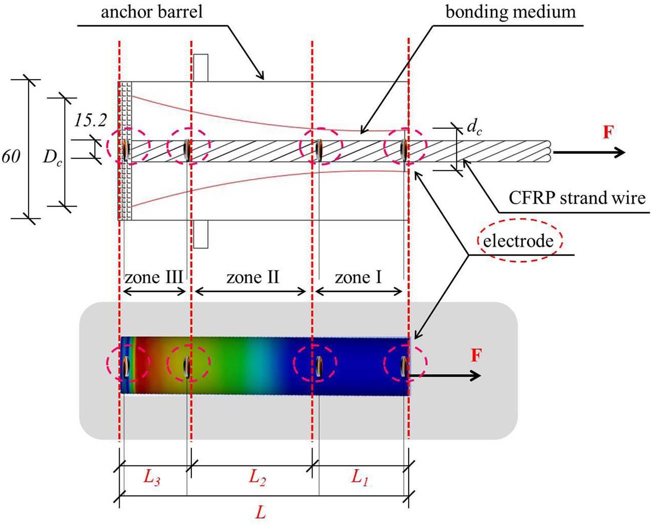
The simulation results show the normal stress distribution in the anchorage zone. The shear stress from the tensile end to the free end changes from a low level to medium and high level [21]. This means the damage distribution in each part of the anchor is not uniform. Thus, the anchorage zone is divided into several monitoring zones, as shown in Figure 10.

Figure 10

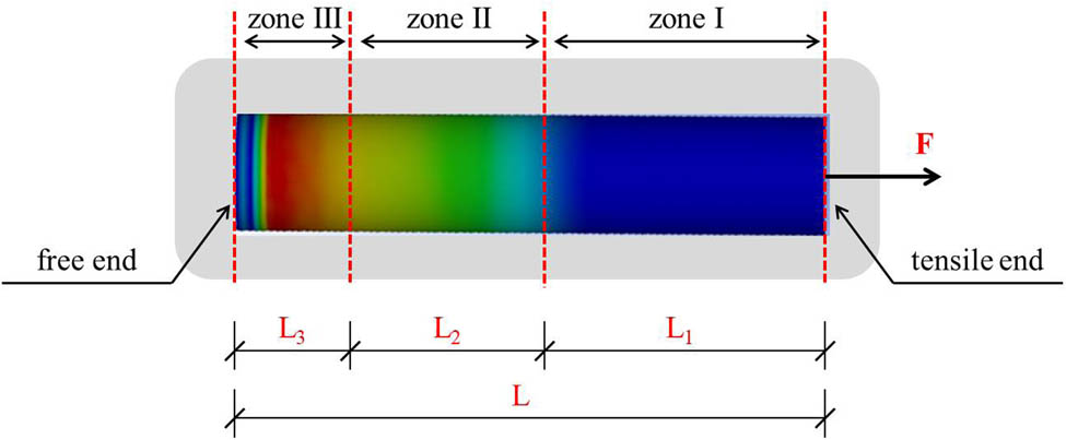
The division of different monitoring areas based on the new-type anchor.

2.3.2 Damage identification theory

Combining the piezoresistive model of the CFRP strand wire (Equation (21)) in Section 2.1 and the damage model of the anchor (Equations (34), (39), (45), (50), (55) and (59)) in Section 2.2, the regional distribution monitoring model of the new-type anchor for the CFRP strand wire is established as follows:

(61) R = 1 + ε x a ε x 2 + b ⋅ L 0 A ε x ∈ E , ε x ∈ E − H − S , ε x ∈ H − S − D ε x ∈ E − H ε x ∈ E − H − S − D ε x ∈ S − D [ zone І − zone III ] ,

where E is the elastic stage, H is the hardening stage, S is the softening stage, and D is the debonding stage.

According to Equation (61), the strain and resistance signals of the CFRP stand wire are measured in different zones for different loading phases.

3 Experimental validation

The regional distribution monitoring model of the anchor is validated by carrying out a series of experimental tests. First, the tests are conducted to examine the volt–ampere characteristics, resistance/resistance fraction–strain relation, and sensitivity of the CFRP strand wire intelligent sensor. Second, the experiments are carried out to measure the ultimate tensile load, anchor efficiency coefficient, displacement, main failure pattern, tensile, and shear distribution of the CFRP strand wire in the anchorage zone for the anchor system. Thereafter, the relationship between the load and both the resistance change and strain was explored.

3.1 Experimental program

The experimental program contains two parts: the CFRP strand wire intelligent sensor and the anchor system.

3.1.1 Materials

The materials of the CFRP strand wire intelligent sensor include the CFRP strand wire, copper foil, electric conductor silver fluid, copper core wire, and epoxy resin. The components of the anchor system include the anchor barrel, CFRP strand wire, and commercial ultra-high performance concrete (UHPC). The specimens and mechanical properties of these materials are shown in Figure 11 and Table 4.

Figure 11

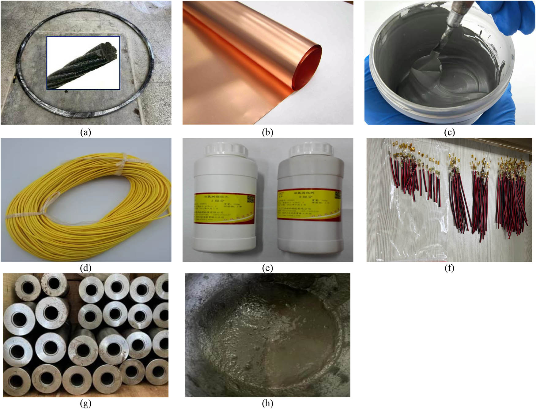
The components of the CFRP strand wire intelligent sensor: (a) CFRP strand wire, (b) copper foil, (c) electric conductor silver fluid, (d) copper core wire, (e) epoxy resin, (f) strain gage, (g) steel barrels, and (h) bonding medium.

Table 4

Parameters of all materials for the CFRP strand wire intelligent sensor

Material	Type	Tensile strength (MPa)	Elasticity modulus (GPa)	Poisson’s ratio	Elongation (%)	Electrical resistivity (Ω m)
CFRP strand wire	HF10-12K	1,800	155 (axial)/10 (radial)	0.27/0.02	1.5	2.6 × 10⁻⁵

Material	Type	Copper content	Thickness (mm)	Electric conductivity
Copper foil	T2	>99.96%	0.09–0.15	>98% IACS

Material	Type	Fineness (μm)	Viscosity (Pa.s)	Resistivity (mΩ)	Adhesion strength (N)
Electric conductor silver fluid	SINMW-3700	≤8	80–280	≤6	≥38

Material	Type	Sectional area (m²)	Electrical resistivity (Ω m)	Electricity (A)
Copper core wire	RVV-0.2	0.2	1.75 × 10⁻⁸	10

Material	Type	Density (g/cm³, 25°C)	Viscosity (cps, 25°C)	Mass ratio
Epoxy resin	AILIK-A/B	A 1.1–1.2/B 0.9–1.0	A 1,000–1,300/B 10–50	100:30

Material	Type	Resistance (Ω)	Sensitivity coefficient	Size (mm)	Monitoring site
Strain gage	BX120-5AA	120 ± 0.1	2.08 ± 1%	3.5 × 4.5	CFRP/Anchor

Material	Type	Elasticity modulus (GPa)	Poisson’s ratio	Tensile strength (MPa)	Brinell Hardness (HB)
Steel barrel	Cr40	211	0.33	≥810	≤207

Material	Type	Elasticity modulus (GPa)	Poisson’s ratio	Compressive strength (MPa)	Water-Binder ratio
UHPC	C120	35	0.19	165	0.2

3.1.2 Specimens

3.1.2.1 CFRP strand wire intelligent sensor

The specimen is shown in Figure 12, and its physical parameters [21] are listed in Table 5.

Figure 12

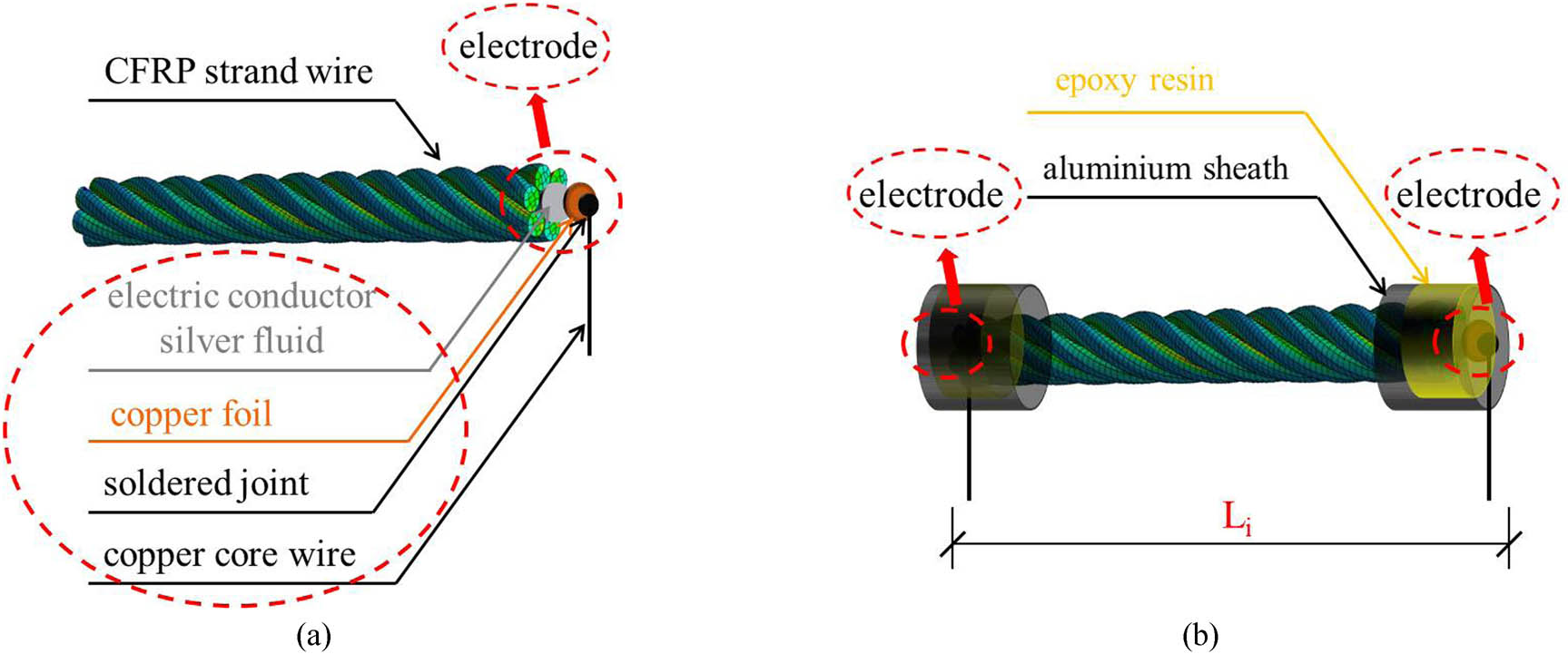
The design diagram of the CFRP strand wire intelligent sensor: (a) design of the electrode, and (b) protection equipment of the electrode.

Table 5

Parameters of the CFRP strand wire intelligent sensor

Order (Li)	Number	Diameter (mm)	Length (mm)	Pitch of the strand wire (mm)
L-300	5	15.2	300	100

The production process was as follows: ① a 150 mm-long CFRP strand wire was chosen, and both ends were polished and cleaned with alcohol; ② the copper foil was cut according to the axial strand size of the CFRP strand wire, and then the copper core wire was welded into and copper foil by tin welding as copper electrode; ③ the copper electrodes were pasted on the two end-sections of the CFRP strand wires with electric conductor silver fluid. A uniform pressure was applied on the copper electrode and cured for 24 h until the conductive silver fluid solidified; ④ the two ends with electrodes of the CFRP strand wire sensor were soaked in epoxy resin, which could protect the electrodes against peeling off after curing; and finally, ⑤ the two aluminum sheaths were bonded to the two electrodes.

3.1.2.2 Anchor system

The specimen is designed as shown in Figure 4, and its geometrical parameters [21] are listed in Table 6. The related parameters of the CFRP strand wire are shown in Table 5. The intelligent monitoring scheme for the anchor system was based on the distributed monitoring technology [18], as shown in Figure 13.

Table 6

Design parameters of the new-type anchor for the CFRP strand wire

Order	Quantity	Anchor length L (mm)	D _b (mm)	D _c (mm)	d _c (mm)	Cone radius (mm)
H300-50-2	5	300	60	50	25	4,800

Figure 13

The experimental specimen of the new-type anchor for the CFRP strand wire.

The production process was as follows: ① the multi-electrodes were installed along the CFRP strand wire; ② the CFRP strand wire was inserted into the vertical barrel and centered by the anchor limiter; and ③ the bonding medium was filled fully in the anchor barrel, with the anchor system gently knocked with a hammer to remove bubbles in UHPC. The anchor specimens were cured for more than a week.

3.1.3 Setup and test methods

3.1.3.1 CFRP strand wire intelligent sensor

The setup and test process are shown in Table 7 and Figure 14.

Table 7

Parameters of all setups

Setup	Type	Working frequency (Hz)	Peak load- tensile (kN)	Peak load- compressive (kN)	Maximum stroke (mm)
Testing machine	YSW-100T	0–100	1,000	1,000	125

Setup	Type	Voltage (mV)	Current (mA)	Resistance (Ω)	Frequency (MHz)
Resistance indicator	VC890D	0–300	0–5	0–10	10

Setup	Type	Resistance of bridge (Ω)	Connection mode	Accuracy (με)	Range (με)	Channel numbers
Strain indicator	TS3862	120	1/4	1	±20,000	16

Figure 14

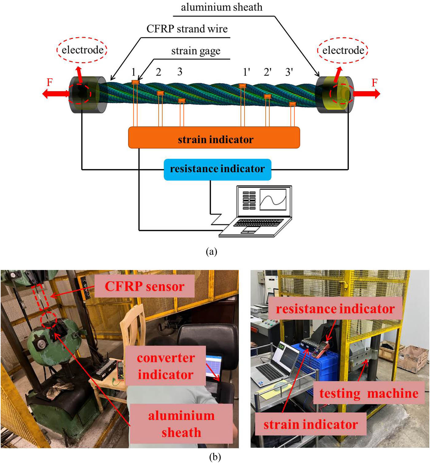
Experimental tests on the CFRP strand wire intelligent sensor: (a) experimental characterization diagram on the CFRP strand wire intelligent sensor and (b) test on the CFRP strand wire intelligent sensor.

The test method is as follows [33,34,35,36,37]: Strain gages were uniformly attached to the off-axial strand (surface of stand wire) within the range of lay. The copper core wires of the CFRP strand wire sensor and strain gages were attached to a strain indicator and a resistance indicator. Preloading was carried out with a load ranging from 1 to 2 kN. According to 20, 40, 60, and 80% of the standard tensile strength of CFRP bars, the load growth rate was maintained at 100 MPa/min. The load of the testing machine remained unchanged for 30 min when the load was close to 80% of the standard value of tensile strength, and then the load gradually increased until the CFRP strand wire sensor was completely damaged. The strain indicator and resistance indicator were used to record the strain and resistance value of the CFRP strand wire sensor, respectively. In order to overcome temperature drift, a small segment of the CFRP strand wire with the same characteristics was connected to the monitoring circuit and used to establish the differential circuit as temperature compensation [27].

3.1.3.2 Anchor system

The setup and test process are shown in Table 8 and Figure 15.

Table 8

Parameters of all setups

Setup	Type	Measurement range (mm)	Measurement accuracy (mm)
Deflection equipment	WCZ-68	0–30	0.001

Setup	Type	Resolution ratio (nm)	Magnification	Accelerating voltage (kV)	Image accuracy (PPI)
Scanning electron microscope	HITACHI	3	×5–×300,000	0.3–30	5,120 × 3,840

Setup	Type	Peak load- tensile (kN)	Torque(N-m)	Maximum stroke (mm)	Torsional angle
Testing machine	MTS809	100/25	1,100/200	150	±50°

Setup	Type	Voltage (mV)	Current (mA)	Resistance (Ω)	Frequency (MHz)
Resistance indicator	ET3100	0–300	0–5	0–10	10

Setup	Type	Resistance of bridge (Ω)	Connection mode	Range (με)	Channel number	Range (με)
Strain indicator	T7116Y	120	1/4	1	16	±20,000

Figure 15

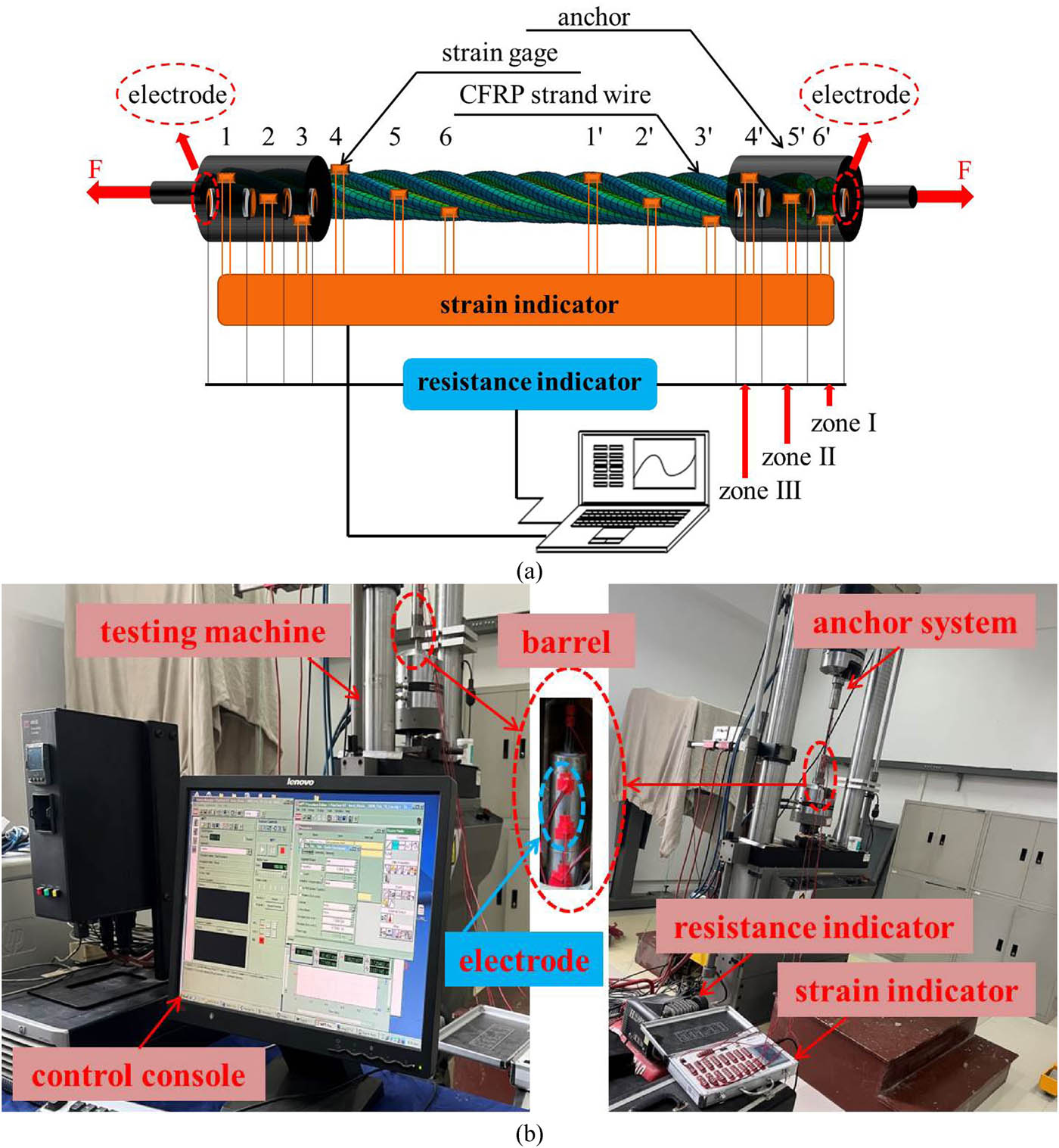
Experimental tests on the new-type anchor for the CFRP strand wire: (a) experimental measurement system, and (b) test on the new-type anchor for the CFRP strand wire.

The test method is the same as in previous studies [33,34,35,36,37].

3.2 Experimental results and analysis

The experimental program contains two parts: the CFRP strand wire intelligent sensor and the anchor system.

3.2.1 Volt–ampere characteristics

The volt–ampere characteristic curve is an important index to measure the electrical stability of conductors. Good volt–ampere characteristics of the CFRP strand wire are the basic premise to realizing stable sensing function. The volt–ampere curve of the CFRP strand wire intelligent sensor is shown in Figure 16.

Figure 16

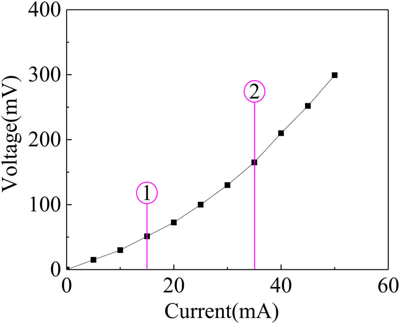
The volt–ampere characteristics of the CFRP strand wire intelligent sensor.

Figure 16 shows that whenever the current increases at the beginning stage (①) and middle stage (②), the trend of current–voltage curve presents almost linear change. This means the CFRP strand wire intelligent sensor follows Ohm’s law and meets the electrical characteristics of Section 2.1.

3.2.2 Resistance/resistance fraction–strain relation

The resistance–strain curve is an important index for sensors since it directly indicates electrical resistance change with the structural strain during tensile loading, as shown in Figure 17.

Figure 17

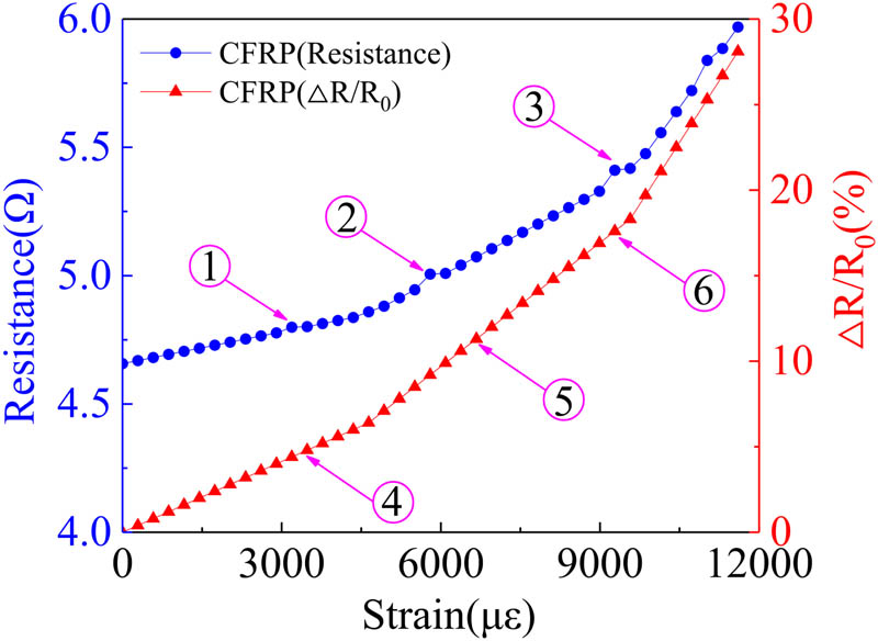
The resistance–strain relation of the P-strand wire intelligent sensor.

Figure 17 shows that when the tensile load is in the elastic stage (①), the carbon fiber tows in the sensor are gradually straightened. The resistance increases slightly in this stage, and the slope of the resistance–strain curve is small. The corresponding resistance and resistance fraction values of the CFRP strand wire intelligent sensor are 4.75 and 4.4%, respectively. When the tensile load is in the plastic stage (②), the carbon fiber tow in the sensor is in a straight state, and the resistance increases. The resistance increases rapidly in this stage, and the slope of the resistance–strain curve is small. The resistance is increased since the carbon fiber is stretched longer. The corresponding resistance and resistance fraction values of the CFRP strand wire intelligent sensor are 5.007 and 9.23%, respectively. The corresponding growth rates are 5.42 and 109.77% between the elastic and plastic stages. When the tensile load enters the last stage (③), the resistance change rate increases significantly, and even intermittent jumps occur in the curve due to the partial fracture of the internal fiber. The resistance increases more sharply, and intermittent jumps appear in the curve due to the fractures of partial carbon fibers. The corresponding resistance and resistance fraction values of the CFRP strand wire intelligent sensor are 5.42 and 17.6%, respectively. The corresponding growth rates are 8.25 and 90.68% between the plastic and last stages. The above results show that the resistance/resistance fraction values of CFRP strand wire sensors are different in different stages, which validates the resistance–strain model proposed in Sections 2.1.2 and 2.1.3.

3.2.3 Sensitivity

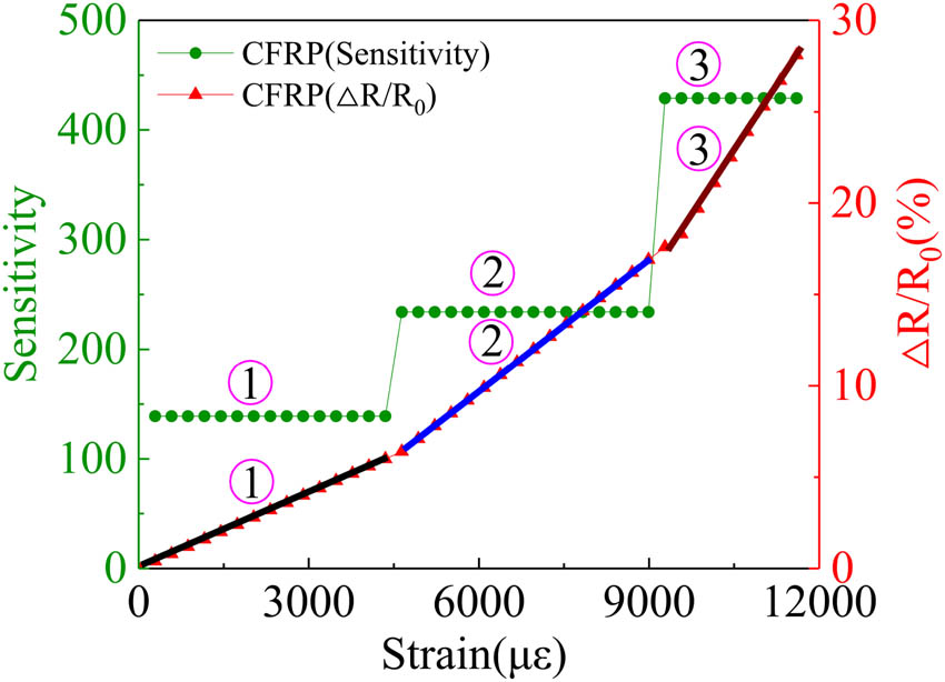
The sensitivity curve is an important index to measure the sensor since it directly indicates the resistance change rate during unit strain. The sensitivity curve calculated by Equation (24) of the CFRP strand wire intelligent sensor is shown in Figure 18, and its corresponding fitting results are listed in Table 9. Meanwhile, the sensitivity comparison between the CFRP strand wire intelligent sensor and other sensors [38,39,40] is listed in Table 10.

Figure 18

The sensitivity of the CFRP strand wire intelligent sensor.

Table 9

Sensitivity fitting results at different stages of the CFRP strand wire intelligent sensor

Stage	Fitted equation	Average sensitivity (k)	Correlation coefficient (R ²)
①	Y = 137.93x + 23.83	137.93	0.973
②	Y = 234.45x – 235.69	234.45	0.956
③	Y = 429.13x – 458.55	429.13	0.974

Note: The micro-strain με was converted into strain ε when the calculated curve slope 1 με = 10⁻⁶ε (%).

Table 10

Comparison of sensitivity between the CFRP sensor and other sensors

Sensor name	Sensitivity range (k)	Measurement range (ε) (%)	Measurement error (%)
CFRP sensor	137.93–429.13	0–1.5	<1
Strain gage	1.8–2.08	0–2	<2
Fiber Bragg grating [38]	1.1–1.4	0–0.5	<2
Soft pneumatic actuator [39]	0–1.85	0–3	<1
Flexible strain sensor [40]	0–294	0–4	<1

Note: The above character refers to the parameters for measuring strain.

Figure 18 shows that when the fitted line is in the elastic stage (①), the corresponding average sensitivity of the CFRP strand wire intelligent sensor is 137.93. Similarly, the corresponding average sensitivities of the CFRP strand wire intelligent sensor in stage (②) and stage (③) are 234.45 and 429.13, which show an obvious three-stage pattern. The reason is that the axial deformation occurring in the elastic stage (①) is relatively small and results in a small change in the resistance change rate, while the CFRP filament entered into the plastic stage after elastic deformation and the axial change is large in this stage (②), which causes the slope (sensitivity) increase. Meanwhile, the CFRP filament entered into the end stage (③) after plastic deformation, and its axial change is large and even causes the slope (sensitivity) to become steep.

As shown in Table 10, the sensitivity of the CFRP sensor is far higher than that of the strain gage, fiber Bragg grating, and soft pneumatic actuator; however, it is lower than that of the flexible strain sensor during stage ① (137.93,294) and ② (234.45,294), and the proportions of reduction are 113.04 and 25.11%. The measurement range of the CFRP sensor is higher than that of fiber Bragg grating and lower than that of the strain gage, soft pneumatic actuator, and flexible strain sensor, and the ratios of higher and lower are 200, 33.33, 50, 100, and 166.66%, respectively. It should be noted that the sensitivity and stability of CFRP sensors vary with the environmental conditions, including temperature and humidity. Calibration is necessary for the sensors under different application scenarios since signal drifts often occur. Special measures should be taken, such as temperature compensation and packaging technologies, to ensure a reasonable sensitivity and stability of CFRP sensors.

3.2.4 Displacement and main failure pattern

The ultimate load was tested to be 247.8 kN on average, and the anchor efficiency coefficient was calculated to be 99.3%. The load–displacement curve and the failure mode are shown in Figure 19.

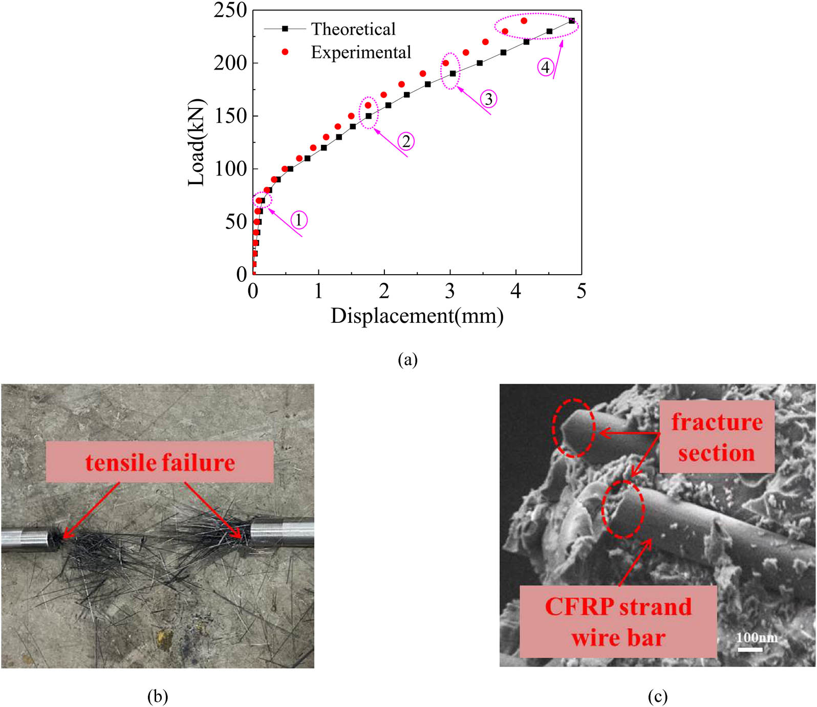
$Figure 19 The load–slip curve and failure process of the new-type anchor for the CFRP strand wire: (a) load–slip curve of the new-type anchor; (b) failure mode of the new-type anchor; and (c) fracture section of CFRP.$

Figure 19

The load–slip curve and failure process of the new-type anchor for the CFRP strand wire: (a) load–slip curve of the new-type anchor; (b) failure mode of the new-type anchor; and (c) fracture section of CFRP.

During the initial loading stage (①), the anchor system is in an elastic state, and displacement increases linearly with load. When the load is over 70.5 kN, the displacement rate (curve slope) tends to become small (①–②), which means the anchor enters the hardening stage. When the load is over 150.6 kN, the displacement curve slope tends to be larger (②–③), which means the anchor is softened and the CFRP strand wire slips in the anchor zone with a slight crackle sound. When the load exceeds 190.2 kN, the displacement rate tends to become large (③–④), which means the anchor starts debonding, and the CFRP strand wire is pulled out finally with crackling. Meanwhile, the debonding zone starts to expand, and the strand wire fractures at 247.8 kN.

From the whole loading process, the experimental ultimate loads in the elastic stage, hardening stage, softening–debonding stage, and failure stage are 70.5, 150.6, 190.3, and 247.8 kN, and the corresponding displacements are 0.14, 1.76, 3.04 and 4.85 mm, respectively. The theoretical displacements based on Equations (34)–(60) are 0.09, 1.51, 2.58, and 4.12 mm, respectively. The contrast results show that the error is within 22.5%, and the proposed model is applicable in illustrating the damage process of the anchor system.

3.2.5 Shear and tensile distribution of the CFRP strand wire in the anchorage zone

The shear stress at the interface between the CFRP strand wire and the bonding medium and the tensile stress distribution of the CFRP strand wire is depicted in Figure 20.

Figure 20

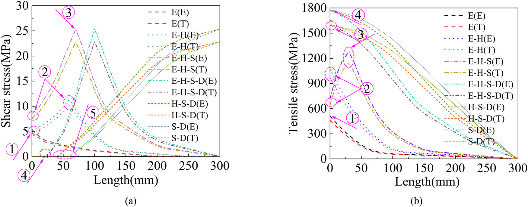
The shear and tensile stress distribution along the new-type anchor: (a) shear stress distribution along the anchor, and (b) tensile stress distribution along the anchor.

It can be seen that when the anchor zone is elastic, the shear stress (Figure 20a, ①) and tensile stress (Figure 20b, ①) increase linearly. When the load increases, the anchor zone enters into a hardening stage. The shear stress (Figure 20a, ②) and tensile stress (Figure 20b, ②) increase at a quicker rate, while x = 50 mm and τ = 15.3 MPa. When the interface between CFRP and the bonding medium starts softening, the shear stress (Figure 20a, ③) reaches a peak value, and x = 76 mm and τ = 25.2 MPa. The length of the softening zone reaches a maximum, and the whole elastic zone of the interface disappears with the disappearance of the softening and debonding regions.

When the load passes the peak value and enters the debonding stage, shear stress (Figure 20a, ④) and tensile stress (Figure 20b, ②–③) would redistribute with the expansion of the debonding zone. When the load increases, the debonding zone continues to increase (Figure 20a, ④–⑤), and tensile stress reaches a peak value (Figure 20b, ④).

The above phenomena indicate that the anchor system goes through an elastic-hardening–softening–debonding stage under tensile loading until final failure. This suggests the applicability of the proposed damage model in analyzing the stress and interface damage in the anchor zone.

3.2.6 Fractional changes in resistance and axial strain

The relationship between the load and both the strain (measured by points 4′, 5′, and 6′ in Figure 15a) and resistance fracture in Zones Ⅰ to Ⅲ (Figure 13) is illustrated in Figure 21.

Figure 21

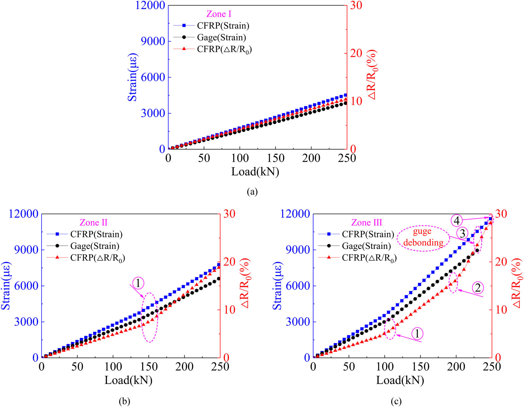
The resistance–strain relation in different zones of the CFRP strand wire under different loads: (a) Zone I, (b) Zone II, and (c) Zone III.

Figure 21 shows that when the load increases from 0 to 70.5 kN, the CFRP strand wire in the three zones is in the elastic stage (Figure 21a–c). A load of 70.5 kN yields the strains of 1,320, 1,122, 2,040, 1,734, 2,640, and 2,244 με, respectively, in Zones Ⅰ to Ⅲ, whereas the corresponding resistance fractures calculated based on Equations (23) and (24) are 3.12, 3.62 and 4.83%, respectively. The comparison of the above data indicates the discrepancies are between 17.65 and 54.81%, respectively, between the results from both methods. When the load is over 70.5 kN (Figure 21c, ①), CFRP strand wire in zone Ⅲ enters into the hardening stage, and it in zones Ⅰ and Ⅱ is still in elastic stage (Figure 21a and b).

When the load increases to over 190.3 kN (Figure 21c, ②), the CFRP strand wire enters into the debonding stage in zone Ⅲ and enters into the softening stage in zone Ⅱ, while it still remains in the hardening stage in zone Ⅰ. A load of 190.3 kN yields strains of 3,466, 2,946, 5,720, 4,862, 8,520, and 7,225 με, respectively, in Zones Ⅰ to Ⅲ, whereas the corresponding resistance change rates calculated based on Equations (24) and (24) are 8.06, 12.35 and 15.38%, respectively. These comparisons indicate the discrepancies are between 18.47 and 90.82%, respectively, between the results from both methods. Meanwhile, only softening and debonding states can be observed at the interface, with gradual expansion of the debonding zone and decrease of the softening zone.

When the load increases to over 220.4 kN (Figure 21c, ③), the resistance does not increase anymore since the strain gages are damaged due to the extrusion between the bonding medium and CFRP strand wire. This phenomenon illustrates the advantage of CFRP self-sensing without the need for external strain gages. When the load is >247.8 kN (Figure 21c, ④), the CFRP strand wire is broken in zone Ⅲ, while in zones Ⅱ and Ⅰ, it is still in the softening or hardening stage. This means the CFRP strand wire in the anchor zone undergoes the elastic–hardening–softening–debonding stage, elastic–hardening–softening stage, and elastic–hardening stage in zones Ⅲ, Ⅱ, and Ⅰ, respectively. Thus, different anchorage zone suffers from varying damages, which makes it necessary to apply the distributed sensing monitoring technology for monitoring the damage in the anchor zone.

4 Conclusions

In this article, the piezoresistive model of the CFRP strand wire, the damage model, and the regional distribution monitoring model of the new-type anchor were established. Meanwhile, the corresponding experiments were carried out. The main conclusions were summarized as follows:

The piezoresistive model of the CFRP strand wire was established based on the electrical and mechanical perspectives, which was verified by the experimental results.
The damage model in the anchorage zone was derived based on the interfacial trilinear model. Following this, the distributions of the shear stress at the interface between the CFRP strand wire and the bonding medium, as well as the normal stress of the CFRP strand wire, were deduced in different loading stages.
The regional distribution monitoring model was established based on the simulation results by using the finite element method. The corresponding regionally distributed resistance and resistance change in the entire anchorage zone were tested and compared with the experimental measurements, which exhibit the constant consistency of the theoretical and experimental results.
The proposed methodology enables self-sensing and self-monitoring on the anchors for the CFRP strand wire in different loading stages by measuring the local resistances in the anchorage zone.
Nevertheless, the sensitivity and stability of the CFRP sensors vary with the environmental temperature and humidity; therefore, special measures should be taken, including temperature compensation and packaging technologies, to guarantee reasonable sensitivity and stability of the CFRP sensors. These considerations are necessary for calibrating the CFRP sensors under different application scenarios.

Acknowledgments

The authors gratefully acknowledge the financial support from the National Natural Science Foundation of China (No. 51478209) and the Science and Technology Service Platform Cultivation Project of Jiangsu Province (No. XQPT202102).

Funding information: Authors state no funding involved.
Author contributions: All authors have accepted responsibility for the entire content of this manuscript and consented to its submission to the journal, reviewed all the results, and approved the final version of the manuscript. Rong-Gui Liu have made substantial contributions to the resource, conception or design of the work; or the acquisition, analysis, or interpretation of data for the work. Zheng-Nan Jing have drafted the work or revised it critically for important intellectual content, and made substantial contributions to the acquisition and analysis.
Conflict of interest: Authors state no conflict of interest.
Data availability statement: All data generated or analysed during this study are included in this published article.

References

[1] Wu G, Chen ZQ, Dang J. Intelligent maintenance of bridges [M]. Beijing: China Communications Press; 2022. p. 115–201.Search in Google Scholar

[2] Wu ZS, Zhang J. Advanced structural health monitoring technology and theory [M]. Beijing: China Science Press; 2015. p. 267–78.Search in Google Scholar

[3] Li L, Sun M, Gong J, Zhou H, Gong F. Evaluating the load-bearing capacity of corroded cables in long-span cable-stayed bridges: A stochastic corrosion field simulation approach. Structure. 2024;65:15–8.10.1016/j.istruc.2024.106650Search in Google Scholar

[4] Liu Y, Gu M, Liu X, Tafsirojjaman T. Life-cycle cost analysis of long-span CFRP cable-stayed bridges. Polymers. 2022;14(9):20–5.10.3390/polym14091740Search in Google Scholar PubMed PubMed Central

[5] Dan DH, Han F, Xu B. Dynamics and intelligent monitoring of complex cable systems [M]. Shanghai: Shang Hai Scientific and Technical Press; 2023. p. 105–208.Search in Google Scholar

[6] Edan A, Abdulsahib W. The impact of using prestressed CFRP bars on the development of flexural strength. Open Eng. 2024;14(1):20240059. 10.1515/eng-2024-0059.Search in Google Scholar

[7] Wang C, Guan S, Sabbrojjaman M, Tafsirojjaman T. Bond performance of CFRP strands to grouting admixture for prestressed structure and development of their bond-slip constitutive models. Polymers. 2023;15(13):2906. 10.3390/polym15132906.Search in Google Scholar PubMed PubMed Central

[8] Kim YJ, Jung WT, Kang JY, Park JS. Testing methods and design specifications for CFRP-prestressed concrete members: A review of current practices and case studies. Case Stud Constr Mater. 2022;16:e00842. 10.1016/j.cscm.2021.e00842.Search in Google Scholar

[9] Qi L, Bai J, Wu H, Xu G, Xiong H, Yang Y. The first engineering application of 10MN CFRP cables in cable-stayed bridge in China. Structure. 2024;68:12–4.10.1016/j.istruc.2024.107199Search in Google Scholar

[10] Tan J. Learn NVH-noise, vibration, modal analysis for beginners and advancements (2nd Edition) [M]. Beijing: China Machine Press; 2021. p. 240–5.Search in Google Scholar

[11] Mei K, Li Y, Wang Y, Li X, Jia W, Sun S. Experimental study and failure mechanism analysis at the meso-scale of the fatigue performance of a CFRP tendon novel composite anchorage. Structure. 2023;58:8–12.10.1016/j.istruc.2023.105449Search in Google Scholar

[12] Han L, Li HL, Wei Y. Conductive Nanocomposite [M]. Beijing: Scientific and Technical Literature Press; 2020. p. 240–5.Search in Google Scholar

[13] Qian RX, Liu YX. Conductive polymer/cellulose fiber composites [M]. Beijing: China Science Press; 2018. p. 267–78.Search in Google Scholar

[14] Lv GY. High performance carbon fibers [M]. Beijing: Chemical Industry Press; 2016. p. 240–5.Search in Google Scholar

[15] Yang GX, Wu LQ. Interface behavior of composite materials [M]. Beijing: Chemical Industry Press; 2020. p. 240–5.Search in Google Scholar

[16] Zhang PX. Fully distributed optical fiber sensing technology [M]. Beijing: China Science Press; 2021. p. 267–78.Search in Google Scholar

[17] Tang SY. Self-sensing FRP materials and intelligent structures based on distributed fiber sensing [M]. Beijing: China Science Press; 2018. p. 267–78.Search in Google Scholar

[18] Jia NB, Piao Y, Song GA. Sensor technology [M]. Nanjing: Southeast University Press; 2007. p. 267–78.Search in Google Scholar

[19] Fang Z, Liang D. Experimental study on bonded anchor with single carbon fiber (CFRP) prestressed reinforcement. J Univ South China. 2004;18(1):35–7.Search in Google Scholar

[20] Mei KH, Zou HX, Sun JS. Analysis and experiment on mechanical performance of CFRP bar bonded anchorage. J Chang’an Univ (Nat Sci Ed). 2017;37(3):64–71.Search in Google Scholar

[21] Liu RG, Jing ZN, Xie GH, Li Y. Mechanical analysis of new-type arc-cone anchor for CFRP strand wires. Compos Struct. 2024;332:16–25.10.1016/j.compstruct.2024.117896Search in Google Scholar

[22] Xie GH, Bian YL, Feng QH, Wang CM, Liu RG. Experimental study on wedge-bonded anchors for CFRP tendons under cyclic loading. Constr Build Mater. 2020;236:117599.10.1016/j.conbuildmat.2019.117599Search in Google Scholar

[23] Xie GH, Feng QH, Tang YS, Liu RG, Bian YL. A fatigue damage model of CFRP tendon bonded anchors. J Jiangsu Univ (Nat Sci Ed). 2019;40(5):603–7.Search in Google Scholar

[24] Conor PC, Owston CN. Electrical resistance of single carbon fibres. Nature. 1969;223(5211):1146–7.10.1038/2231146b0Search in Google Scholar

[25] Xu HZ. Research on carbon fiber composite self-sensing performance of prestressed concrete structure [D]. Zhenjiang: Jiang Su University; 2016. p. 22–30.Search in Google Scholar

[26] Le XZ. Study on carbon nanofibers composite material’s resistance-strain sensor property [D]. Wuhan: Wuhan University of Technology; 2007. p. 38–42.Search in Google Scholar

[27] Liu D. Sensing properties of resin based carbon fiber reinforced bar and its application in pre-stressed concrete structure [D]. Zhenjiang: Jiang Su University; 2020. p. 67–71.Search in Google Scholar

[28] Yang J. Study on the bridge damage identification and monitoring system based in distributed long-gage FBG sensing [D]. Nanjing: Southeast University; 2021. p. 43–7.Search in Google Scholar

[29] Xu LZ. Elasticity [M]. Beijing: Higher Education Press; 2008. p. 105–8.Search in Google Scholar

[30] Chen J, Cheng SS. Fracture mechanics [M]. Beijing: Science Press; 2006. p. 35–48.10.1016/j.corsci.2005.02.014Search in Google Scholar

[31] Zhang JY, Li QY. SolidWorks 2014 Chinese version basic design [M]. Beijing: Tsinghua University Press; 2015. p. 35–9.Search in Google Scholar

[32] Wang MX. ANSYS numerical analysis of engineering structure [M]. Beijing: China Communications Press; 2016. p. 25–9.Search in Google Scholar

[33] JT/T775-2016. Transportation industry standard of the People’s Republic of China Cable of parallel steel wires for large-span cable-stayed bridge [S]. Beijing, China: Ministry of Transport of the People’s Republic of China Press; 2016.Search in Google Scholar

[34] JGJ85-2010. Industry standard of the People’s Republic of China Technical specification for application of anchor, grip and coupler for prestressing tendons [S]. Beijing, China: China Building Industry Press; 2010.Search in Google Scholar

[35] ASTM:D3552. Standard test method for tensile properties of fiber reinforced metal matrix composites [S]. Philadelphia, USA: American Society for Materials and Testing; 2007.Search in Google Scholar

[36] GB/T30826-2014. Industry standard of the People’s Republic of China Technical conditions for steel strand cable of cable styed bridge [S]. Beijing, China: General Administration of Quality Supervision, Inspection and Quarantine of the People’s Republic of China; 2014.Search in Google Scholar

[37] ASTM:D3039. Standard test method for tensile properties of polymer matrix composite materials [S]. Philadelphia, USA: American Society for Materials and Testing; 2014.Search in Google Scholar

[38] Zhang Z, Wei S, Nan H. Experimental study of type-I crack propagation in rock monitored by fiber Bragg grating. Theor Appl Fract Mechaincs. 2024;134:11–3.10.1016/j.tafmec.2024.104734Search in Google Scholar

[39] Chen H, Ali MA, Wang Z. Performance optimizing of pneumatic soft robotic hands using wave-shaped contour actuator. Results Eng. 2024;103:2–3.10.2139/ssrn.4966317Search in Google Scholar

[40] Lv R, Cao X, Zhang T. A highly stretchable, self-healing, self-adhesive polyacrylic acid/chitosan multifunctional composite hydrogel for flexible strain sensors. Carbohydr Polym. 2024;123:21–4.10.1016/j.carbpol.2024.123111Search in Google Scholar PubMed

Received: 2024-10-14

Revised: 2024-12-16

Accepted: 2025-01-25

Published Online: 2025-04-12

This work is licensed under the Creative Commons Attribution 4.0 International License.

Articles in the same Issue

https://doi.org/10.1515/secm-2025-0051

Keywords for this article

anchor; CFRP strand wire; piezoresistive model; damage model; regional distribution monitoring

Creative Commons

BY 4.0