An application of Nwogu’s Boussinesq model to analyze the head-on collision process between hydroelastic solitary waves

1 Introduction

During the past few years, hydroelasticity grabbed the attention of different researchers due to its versatile applications in engineering as well as in various industrial processes. Hydroelasticity is associated with the motion and deformation of elastic bodies responding to a hydrodynamic excitation, and associated response to the movement of a working fluid. Hydroelastic waves can be observed in those colder areas, where frozen water is transformed into runways, and roads, and automobiles are helpful to break the ice. Particularly, nowadays industries are getting in deeper offshore and polar regions and are facing different challenges in design and modeling. The mathematical methods and theory of hydroelasticity relevant to convoluted problems are not adequately developed.

The hydroelastic problems are coupled in such a way that the deformation of elastic bodies relies upon hydrodynamic forces and vice versa. In such kind of problems, coupled fluid motions are very much complicated to studied numerically and theoretically. Therefore, various authors investigated the mechanism of hydroelasticity in different geometrical aspects using multiple mathematical methods. For instance, Ertekin et al. [1] investigated the waves due to a moving disturbance in a finite channel using the shallow water approximation. They used the Green–Naghdi theory to analyze the behavior of moving pressure on the surface of an elastic plate. Xia and Shen [2] discussed the nonlinear interaction between water and a floating ice sheet with compressive force effect. An analytical method has been used to obtain the solution of a periodic equation. They found that the wave speed, shape and wavelength of the nonlinear waves depend on the wave amplitude. Bennetts et al. [3] addressed the scattering of linear wave under an ice sheet having variable thickness buoyant on a variable quiescent depth. They used the Rayleigh–Ritz technique with a combination of variational principle and multi-mode approximation to determine the velocity potential. Deike et al. [4] presented an experimental analysis of linear and nonlinear hydroelastic waves, propagating under an ice sheet in the presence of surface tension. They used an optical technique to determine the full time and space field. Wang and Lu [5] discussed the propagation of nonlinear hydroelastic waves in two dimensions. Wang et al. [6] scrutinized the impact of longitudinal compressive force response of a thin beam of a rectangular cross-section on the surface of the water. Cheng et al. [7] presented a two-dimensional model to analyze the interaction between an elastic plate and monochromatic waves in a finite channel having variable depth. They used the Euler–Bernoulli–von Karman nonlinear beam model to examine the imposed fluid pressure on the fluid–structure interface. Recently, Trichtchenko et al. [8] discussed the stability of periodic traveling waves in the presence of thin elastic plate in a two-dimensional channel using an asymptotic method. Parau and Dias [9] studied the nonlinear hydroelastic steady response of infinite broken ice sheet in the presence of a moving load.

It is renowned that the Korteweg–de Vries (KdV) equation is helpful to describe long-time asymptotic weakly nonlinear shallow water waves. Initially, Gardner et al. [10] introduced an inverse scattering transform (IST) method to obtain the exact solution for the KdV equation. Further, they presented the essential characteristics of collision process between solitary waves. When the collision occurs between solitary waves, they exchange their positions, energies and regain their original forms after separation. During this whole process, solitary waves have extraordinarily stable entities and maintain their original shapes throughout the interaction process. However, the sole impact of a collision is their phase shifts. It is now realized that the striking and colliding features of solitary waves can maintain in a conservative system. The IST method depicts that all the KdV solitary waves propagate along the same direction with their corresponding boundary conditions showing disappearing elevations at infinity [10, 11, 12]. For overtaking collision between solitary waves, one can efficiently use the IST method to obtain the behavior of solitary waves during colliding. To determine the head-on collision between solitary waves, however, it is compulsory to utilize the asymptotic expansion to solve the original field equations. For this purpose, the Poincaré–Lighthill–Kuo (PLK) method is an excellent and efficient technique to determine the head-on collision process between solitary waves. Su and Mirie [13] discussed the head-on collision process between solitary gravity waves using the PLK technique, and presented the solution up to fourth order approximation. Dai [14] examined the interaction between solitary waves in a two-layer fluid regarding a generalized form of Boussinesq’s equations, and obtained the second order series solution by using the PLK method and a reductive perturbation method. Mirie and Su [15, 16] reported the head-on collision among generalized and modified solitary waves using the PLK method. They considered a two-layer fluid model in a finite channel which is bounded above and below by a rigid sheet. After few years, Zhu and Dai [17] investigated the generalized KdV solitary waves and their head-on collision process in the presence of surface tension effects. Later, Zhu [18] considered the similar problem and used the same methodology to obtain the modified KdV solitary waves to examine the head-on collision process with surface tension effects. Recently, Ozden and Demiray [19] elaborated the work of Su and Mirie [13] under the assumption of different trajectory functions. The order of trajectory function assumed by Su and Mirie [13] is ε, where ε is the perturbation parameter related to the wave amplitude. Ozden and Demiray [19] assumed, with the same definition for ε, the order of trajectory functions is ε².

Nonlinear waves in shallow water have been studied based on the Boussinesq model. For the broader range of water depth, Nwogu’s Boussinesq model [20] is beneficial. This model, proposed by Nwogu [20] in 1993, is not only limited for shallow water waves, but it is also applicable for deep water waves,which have been examined numerically by Wei et al. [21] and Wei and Kirby [22]. Later, Zhang et al. [23] described the mathematical properties of a Boussinesq model having constant depth for weakly nonlinear and weakly dispersive water waves. They found that the 1 + 1 dimensional Boussinesq model does not hold the Painleve integrability. Chen et al. [24] discussed the head-on collision among solitary waves using Nwogu’s Boussinesq model. They discussed the head-on collision process at a constant depth by using the PLK method.

Recently, Bhatti and Lu [25] discussed the head-on collision process among two nonlinear hydroelastic solitary waves in the framework of potential flow theory. They also used the PLK method in order to obtain the series solution and derived a third-order KdV for the hydroelastic wave profile. Unfortunately, it does not seem applicable for deep water waves, because the Taylor series used to derive the governing equations fails to converge at infinity. However, the present study is also appropriate for deep water waves as well as for shallow water waves.

According to the authors’ best knowledge, no such attempt has been made on the head-on collision between hydroelastic solitary waves by using Nwogu’s Boussinesq model through a shallow water depth. It has been proved by Il’ichev [26] that solitary waves of sufficiently small amplitude exist on the water–ice interface. Therefore, the main theme of the present investigation is to analyze the head-on collision process between hydroelastic solitary waves having a long wavelength and a small amplitude in terms of Nwogu’s Boussinesq model. This model consists of a free parameter α that is associated with horizontal velocities, according to the selected level of horizontal velocity variables. This parameter provides more freedom to determine different problems for multiple values of α. We have considered a thin elastic plate on the surface of the water. To solve the problem analytically, we employ the PLK method and present the solution up to the third order approximation. The present model is applicable for different values of the mean depths. The physical features of all the parameters are discussed graphically and mathematically for plate deflection, phase shift, maximum run-up at the time of collision, wave speed, and distortion profile.

2 Governing equations

Consider two hydroelastic solitary waves traveling beneath an infinite elastic plate in shallow water. A Cartesian coordinate system (x, z_α) is taken with the x-axis taken along the horizontal direction and the z_α-axis measured upwards from the still-water level. A thin elastic plate is taken on the surface of water. The deflection of the plate (namely the hydroelastic wave profile) is presented by z_α = ζ (x, t). z_α = −h(x) is the bottom of the channel, and z_α = 0 is the undisturbed plate–water interface. The fluid is considered to be incompressible and inviscid, the flow is irrotational, and there is no cavitation between an elastic plate and water. The governing equations in terms of Nwogu’s Boussinesq model can be written as [20]

In the above equations, U is the velocity vector at an arbitrary depth z_α, g the gravitational acceleration, ρ the density of the fluid, and P_e the pressure on the plate–water interface. The detailed derivation for the terms with z_α in Eqs. (1) and (2) was elaborated by Nwogu [20].

For a thin homogeneous elastic plate with a uniform mass density ρ_e and a constant thickness d, the relationship between a plate deflection ζ and the pressure P_e consists on the Euler–Bernoulli beam theory which can be written as

where D = Ed³/[12(1 − ν²)], M = ρ_ed, ν Poisson’s ratio, and E Young’s modulus of the plate. Q is associated to the lateral stress of the plate (with compression at Q > 0).

We consider one-dimensional flow in a channel of constant depth, namely U = {U(x, t), 0, 0} and the water depth h is constant. Nwogu’s Boussinesq model for hydroelastic waves in the flow field U = {U(x, t), 0, 0} can be written as

where

and α is a free parameter representing the depth level.

According to Nwogu’s Boussinesq model [20], it is observed that if the velocity at depth z_α = −0.531h is used, then the corresponding dispersion relation can be enhanced to that obtained by the classical potential flow theory. The free parameter α is helpful to analyze various kinds of problems. For instance by taking α = 0, Eqs. (4) and (5) reduce to the classical Boussinesq equation. Further, for α = −1/3 or −1/2, one can get two different models and the associated field U shows the depth-mean and bottom velocities, respectively. Depth-mean system is almost equivalent to the system at a water depth with α = −1/3. It is worth mentioning here that the present results can reduce to the results obtained by Chen et al. [24] for pure-gravity waves by taking D ! 0, Q ! 0 and M → 0 in Eqs. (4) and (5).

3 Solution methodology

We will apply the PLK method in the subsequent section. Let us introduce the following coordinate transformations in wave frame as follows

where η₀ and ξ₀ represent the left- and right-going phase variables, respectively; δ is a positive constant; k̄ and k are the wave numbers of order unity for the left- and right-going wave, respectively; ε with 0<ε ≪ 1 is a dimensionless parameter, which represents the wave amplitude and order of magnitude; C and C̄ are the wave speeds of right-and left-going solitary waves. Introducing the transformation of phase functions with wave frame coordinates, we write

In the above equation, θ(ξ , η) and φ(ξ , η) are the phase functions to be deduced in the perturbation analysis of Eqs. (4) and (5). The purpose of these functions is to make the asymptotic approximations, which acquiesce us to analyze the phase changes due to a collision.

In our present study we consider δ = 1/2 in Eq. (7) for the scaling of the horizontal wavelength by using Ursell’s relationship. The purpose of δ = 1/2 is to derive the KdV equation for shallow water solitary waves. However, δ = 0, 1/4, 1/8, 1 are also applicable, but these values have some limitations in our present case. For instance, these values fail to give the KdV equation. On the other hand, these values are beneficial to derive different forms of KdV equations for internal solitary waves in a two-layer fluid model using the PLK method. Mirie and Su [16] and Zhu [18] used δ = 1 to derive the modified KdV equation for a two-layer fluid model. Zhu and Dai [17] used δ = 1/4 to derive the generalized form of KdV equation for a two-layer fluid model. Furthermore, Dai et al. [27] used δ = 0 to discuss the head-on collision between solitary waves propagating in a compressible Mooney–Rivlin elastic rod. An interesting fact is that they derived a KdV equation for the solitary waves in a single-layer fluid model. Therefore, the value of δ is important and mainly depends upon mathematical and physical assumptions of the governing problem.

Let c(k) be the phase speed

where

By taking D = 0, Q = 0 and M = 0, the phase speed in Eq. (9) reduces to that for pure-gravity waves obtained by Nwogu [20]. For the sake of simplicity, we introduce a column vector T defined as

In view of the PLK technique, one can describe the following series expansions

where c̄ = c(k̄), and in the right-hand side of Eqs. (12) to (16), the variables with subscripts will be determined throughout the singular perturbation analysis; a and b are the amplitudes.

4 Perturbation analysis

Using the asymptotic expansion in Eqs. (12) to (16), we obtain a set of coupled differential equations in the coefficients form of ε32,ε52,ε72,… which are expressed in a sequence as follows.

4.3 Coefficients of ε^7/2

In the third order equations, one obtains the following set of equations

(41) N k ∂ T 3 ∂ ξ + a c k F 1 + 1 h F 2 A + 1 h 2 F 3 A 2 A ′ + 1 h F 4 A ′ A 1 + A A ′ 1 + F 5 A ′ 1 + F 6 A ′ ′ ′ 1 + F 7 + F ~ 8 A ′ + N ~ k ¯ ∂ T 3 ∂ η + b c k ¯ F ~ 1 + 1 h F ~ 2 B + 1 h 2 F ~ 3 B 2 B ′ + 1 h F ~ 4 B ′ B 1 + B ′ 1 B + F ~ 5 B ′ 1 + F ~ 6 B ′ ′ ′ 1 + F ~ 7 + F 8 B ′ = 0 ,

where N and Ñ are defined in Eq. (18) while F_n and F̃_n (n = 1 . . . 8) are listed in Appendix A.

Let’s assume the solution of the following form

(42) T3=X2(ξ,η)R+Y2(ξ,η)R˜,

where X₂(ξ , η) and Y₂(ξ , η) are two functions to be determined. Using Eq. (42) in Eq. (41), and multiplying it by L, we get the equation for X₂. The procedure is similar to that from Eq. (22) to Eq. (24). The resultant equation is further divided into three groups, namely (i) secular terms, (ii) local terms and (iii) non-local terms.

4.3.1 Secular terms

The secular terms appearing in this order are found as

(43) L F 1 + 1 h L F 2 A + 1 h 2 L F 3 A 2 A ′ + 1 h L F 4 A ′ A 1 + A A ′ 1 + L F 5 A ′ 1 + L F 6 A ′ ′ ′ 1 .

The above equation can be written in a simplified form as

(44) A 1 ‴ − A 1 ′ + 3 h A 1 A ′ + A 1 ′ A + − 2 c 2 + C 14 A ′ − C 15 h A A ′ − C 16 h 2 A 2 A ′ ,

where C₁₄, C₁₅ and C₁₆ are defined in Appendix B. Upon integrating the above equation we get

(45) A 1 ″ − A 1 + 3 h A 1 A = ( 2 c 2 − C 14 ) A + C 15 2 h A 2 + C 16 3 h 2 A 3 .

In the above equation, the first term on the right side reveals a secular behavior which is unbounded as ξ ➝ ±∞, and as a result, the series solution will not be asymptotic. Therefore, the term in the coefficient must vanish. Let

(46) c 2 = C 14 2 .

Then the solution of Eq. (45) can be written as

(47) A 1 = C 17 A + C 18 h A 2 ,

where C₁₇ and C₁₈ are defined in Appendix B.

In Eq. (47), the homogeneous solution in the form of A⁰ is not written. Because, as going to higher order approximation it is found that the homogeneous solution only causes a uniform shift in the wave profile at the origin of ξ, which expresses a simple phase shift as mentioned above. Therefore, this term is dropped here.

Similarly, one has

(48) B 1 = C 17 B + C 18 h B 2 ,

(49) c ¯ 2 = C 14 2 .

This completes the solutions for Eqs. (38) and (40).

4.3.2 Non-local terms

The non-local terms appear in this order are found as

(50) L F 7 A ′ = 0.

The above equation reduces to

(51) θ 1 = θ ¯ 1 , 0 k ¯ h ∫ − ∞ η B d η 1 + θ ¯ 1 , 1 k ¯ h 2 ∫ − ∞ η B 2 d η 1 ,

where

(52) θ ¯ 1 , 0 = − b 2 Y C 2 + χ C 5 + a h C 3 + χ C 6 A ,

(53) θ ¯ 1 , 1 = − b 2 2 Y C 4 + χ C 7 .

Similarly

(54) φ 1 = φ ¯ 1 , 0 k h ∫ + ∞ ξ A d ξ 1 + φ ¯ 1 , 1 k h 2 ∫ + ∞ ξ A 2 d ξ 1 ,

where

(55) φ ¯ 1 , 0 = − a 2 Y C 2 + χ C 5 + b h C 3 + χ C 6 B ,

(56) φ ¯ 1 , 1 = − a 2 2 Y C 4 + χ C 7 .

In Eqs. (51) and (54), one can observe that all the terms reveal a simple phase shift as compared with the first-order phase shift. However, only one term in θ ¯ 1 , 0 and φ ¯ 1 , 0 depends on ξ and η as η ➝ +1 and ξ v −∞ (see Eqs. (52) and (55)). Therefore, θ₁ and φ₁ enter into the argument of ξ and η of the functions A and B. The functions A and B distort the wave profile, and as a result, the wave profile is different before and after collision process. It is found that the wave profile tilts backward in the direction of wave propagation (see Fig. 12). However, Bhatti and Lu [25] observed the similar behavior for hydroelastic wave profile as well as Su and Mirie [13] also found that the wave profile tilts backward for pure-gravity wave profile. The behavior of solitary waves before collision process also remains the same as compared with Su and Mirie [13] and Bhatti and Lu [25].

Figure 1

Three-dimensional view of head-on collision between two solitary waves versus time t.

Figure 2

Head-on collision between two solitary waves for different values of Γ and ff. Black line (Chen et al. [24]): Γ = 0, σ = 0, Λ = 0; Green line: Γ = 0.49; Blue line: Γ = 0.62; Red line: Γ = 0.82.

Figure 3

Head-on collision between two solitary waves for different values of α. Black line: α = 0; Green line: = −1/5; Blue line: α = −1/2; Red line: α = −4/5.

Figure 4

Head-on collision between two solitary waves for different values of h. Black line: h = 1; Green line: h = 4; Blue line: h = 7; Red line: h = 10.

Figure 5

Comparison of Head-on collision between two hydroelastic solitary waves. Green line: Bhatti and Lu [25]; Red line: Present results. Solid line: Γ = 0.03; Dashed line: Γ = 0.24.

Figure 6

Maximum run-up vs wave amplitude for different values of α. Black line: α = 0; Green line: = −1/3; Blue line: α = −2/5; Red line: α = −2/3.

Figure 7

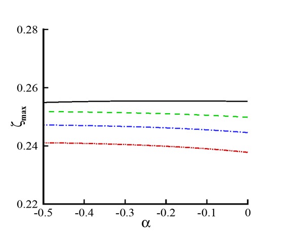
Maximum run-up vs free parameter α. Black line: Γ = 0; Green line: Γ = 0.24; Blue line: Γ = 0.36; Red line: Γ = 0.48.

Figure 8

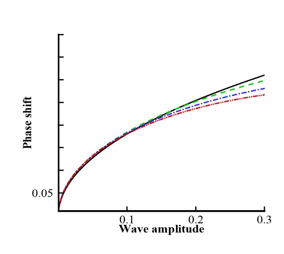
Phase shift vs wave amplitude for different values of α. Black line: α = −3/10; Green line: = −13/20; Blue line: α = −4/5; Red line: α = −9/10.

Figure 9

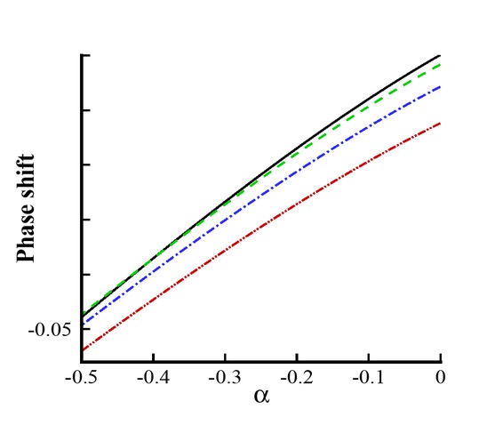
Phase shift vs free parameter α. Black line: Γ = 0.008; Green line: Γ = 0.02; Blue line: Γ = 0.04; Red line: Γ = 0.09.

Figure 10

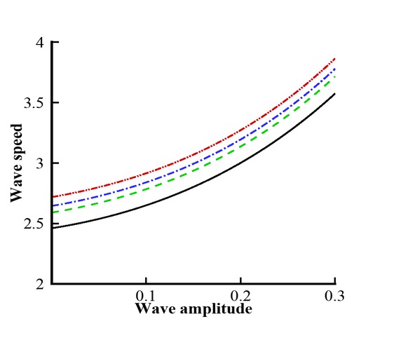
Wave speed vs wave amplitude for different values of α. Black line: α = 0; Green line: = −3/10; Blue line: α = −1/2; Red line: α = −9/10.

Figure 11

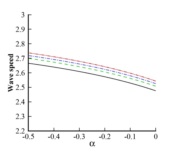
Wave speed vs free parameter α for different values of Γ. Black line: Γ = 0; Green line: Γ = 0.24; Blue line: Γ = 0.36; Red line: Γ = 0.48.

Figure 12

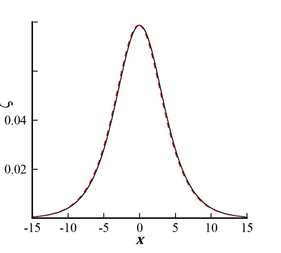
Distortion profile. Black line: Before collision; Red line: After collision.

4.3.3 Local terms

The local terms appearing in the above equations are summarized as

(57) L N ~ R k ¯ ∂ X 1 ∂ η + b c k ¯ L F 8 + L F ~ 1 + 1 h L F ~ 2 B + 1 h 2 L F ~ 3 B 2 B ′ + L F ~ 4 B ′ B 1 + B ′ 1 B + L F ~ 5 B ′ 1 + L F ~ 6 B 1 ‴ + L F ~ 7 B ′ + a c k L F ~ 8 A ′ = 0 .

After integration, one can obtain the solution in the following form

(58) X 2 ( ξ , η ) = C 19 B + C 20 B 2 + C 21 B 3 + A 2 ( ξ ) ,

where C₁₉, C₂₀ and C₂₁ are defined in Appendix B. Similarly

(59) Y 2 ( ξ , η ) = C 19 A + C 20 A 2 + C 21 A 3 + B 2 ( η ) .

In the above equations A₂(ξ) and B₂(η) are the undetermined functions. For further analysis, calculations are stopped and the solutions of A₂(ξ) and B₂(η) are omitted here.

5 Analytical results

The resulting solutions in the foregoing sections are combined and presented below.

The surface elevation at the fluid–plate interface can be described by means of Eqs. (21) and (23), and one gets

where X₁(ξ , η) and Y₁(ξ , η) are defined in Eqs. (38) and (40), respectively.

The distortion profile can be calculated with the help of Eq. (60). Therefore, those terms, which are the products of B(η) and A(ξ) in Eq. (60) must disappear. Thus, the distortion profile at the fluid–plate interface can be obtained. It can be written by setting B(η) = 0. One obtains

The maximum run-up ζ_max while collision at the plate–water interface can be obtained by taking A = B = 1 in Eq. (60). Thus,

The velocity U at the bottom of the channel can be achieved from Eqs. (21) and (23), and one has

The asymptotic results for the wave speeds can be obtained by means of Eqs. (26) and (46), then one has

The phase shifts at the time of collision process read

where θ₀, θ₁, φ₀, and φ₁ are given in Eqs. (34), (36), (51), and (54), respectively.

6 Graphical results and discussion

This section is associated with the graphical results of all the pertinent parameters involved in the governing flow problem. Figures 1 to 12 have been sketched for the head-on collision, phase shift, maximum run-up amplitude, wave profile, and distortion profile. The following values have been chosen to generate the graphical results: h = 1, g = 9.8ms⁻², Γ = 0.24, σ = 0.05, α = −1/3, ν = 0.50, ρ_e = 917 kgm⁻³, ρ = 10³ kgm⁻³, and Λ = 1.

Figure 1 represents the three-dimensional sight of a head-on collision among two solitary waves versus time t.

One can notice that the wave speed and the magnitude of solitary waves are similar before and after a collision. Further, similar behavior was observed by Bhatti and Lu [25]. Figures 2 to 5 show the two-dimensional view of head-on collision for multiple values of Γ, σ, h, and α. In Figure 2 one can notice that when the elastic plate parameter Γ increases, the amplitude of both solitary waves decreases significantly. The plate term Γ, as shown in Eq. (10), is directly proportional to Young’s modulus E and the constant thickness of plate d. Young’s modulus is described as the relationship between stress and strain in a material. Physically,when Young’s modulus increases, the plate becomes stiffer, and opposing forces occur, which tends to suppress the wave profile. It is worth mentioning here that when Γ ➝ 0, σ ➝ 0 and Λ ➝ 0, the present results reduce to those for pure gravity waves obtained by Chen et al. [24].

Figure 3 is plotted against different values of the free parameter α. For α = 0 the results are similar to the classical Boussinesq equation. However, when α increases, a tilting occurs in the wave profile and the wave amplitude slightly increases. Figure 4 shows the variation of water depth h on the wave profile. This model is applicable for deep water waves as stated in the preceding sections. However, the results obtained by Bhatti and Lu [25] for a head-on collision between hydroelastic solitary waves by using classical Boussinesq equation are not applicable for deep water waves. Bhatti and Lu [25] derived the mathematical formulation using the Taylor series expansion at the bottomboundary conditions of finite depth. However, the Taylor series fails to converge at infinity condition. It can be viewed from Figure 4 that an increment in h creates a significant enhancement in the wave profile. Figure 5 shows the comparison of the wave profile with previously published results presented by Bhatti and Lu [25] for shallow water waves. In Figure 5, one can see that the wave profiles for Nwogu’s fluid model are much narrower, while the wave profiles are much flatter in shallow water model as shown by Bhatti and Lu [25].

Figures 6 and 7 are plotted to see the maximum run-up amplitude during the head-on collision. Figure 6 shows the maximum run-up versus the wave amplitude during collision process. It depicts from Figure 6 that when the free parameter α increases, the maximum run-up amplitude increases. Figure 7 shows the variation of maximum run-up amplitude versus α. In this figure, we can see that the behavior of maximum run-up amplitude is uniform for both pure-gravity and hydroelastic wave profiles. However, the maximum run-up amplitude reduces in the presence of thin elastic plate.

Figures 8 and 9 represent the phase shift profile against different values of the plate parameter Γ and the free parameter α. From Figure 8 one can observe that when α increases, the phase shift profile changes its behavior. It decreases due to an increment in α. Figure 9 represents the variation of phase shift profile versus α. In this figure, one can see that the behavior is uniform throughout the domain, whereas the magnitude is small in the presence of hydroelastic wave profile. Figures 10 and 11 represent the wave speed against different values of Γ and α, respectively. It depicts from Figure 10 that wave speed increases due to significant effects of α. Figure 11 is plotted for the wave speed versus α. In this figure, one can see that along the whole domain of α, the phase shift is uniform but increases due to a great influence of elastic plate.

Figure 12 shows the distortion profile before and after collision process. Before collision process the wave profile is symmetric. However, when the distortion occurs in the wave profile, it tilts backward in the direction of wave propagation, and the wave profile becomes unsymmetric.

7 Conclusions

The head-on collision between hydroelastic solitarywaves beneath a thin elastic plate floating on the surface of water has been studied. The problem is formulated with the help of Nwogu’s Boussinesq model. This model consists of a free parameter α that is associated with horizontal velocities according to the chosen level of horizontal velocity variables. The modeled equations are nonlinear, and the exact solution for such kind of nonlinear differential equations are difficult to obtain. Therefore, the Poincaré–Lighthill–Kuo method to get the analytical series solution for the governing differential equations have been applied. The head-on collision process between two solitary waves under a thin elastic plate is mainly determined. The physical features of all the governing parameters is presented and discussed with the help of graphs. The novelty of the present methodology is compared with previously published results.

It is found that when the free parameter α increases, it creates a minor tilting on both waves and causes a slight increment in both waves. However, the collision process does not cause any significant impact on the wave profiles, which regain their original shapes after separation. It is also observed that the presence of elastic plate causes a marked reduction in the amplitude of the solitary waves. Moreover, it is noticed that the maximum run-up amplitude decreases due to a higher impact of plate effects whereas an opposite behavior has been observed for the free parameter α. Further, it has been found that the phase

shift tends to decrease due to the increment in the free parameter α. Distortion profile shows that the solitary waves tilt backward after the collision process in the direction of wave propagation, however, before collision process the wave remains symmetric. It is worth mentioning here that the present results also reduce to those for the pure-gravity waves obtained by Chen et al. [24] by taking Λ ➝ 0, Γ ➝ 0 and σ ➝ 0 in the dynamical boundary conditions. Moreover, the results for the classical Boussinesq model can also be recovered by taking α = 0.

References

[1] Ertekin R. C., Webster W. C., Wehausen J. V., Waves caused by a moving disturbance in a shallow channel of finite width, J. Fluid Mech., 1986, 169, 275-292.10.1017/S0022112086000630Suche in Google Scholar
[2] Xia X., Shen H. T., Nonlinear interaction of ice cover with shallow water waves in channels, J. Fluid Mech., 2002, 467, 259-268.10.1017/S0022112002001477Suche in Google Scholar
[3] Bennetts L. G., Biggs N. R. T., Porter D., A multi-mode approximation to wave scattering by ice sheets of varying thickness, J. Fluid Mech., 2007, 579, 413-443.10.1017/S002211200700537XSuche in Google Scholar
[4] Deike L., Bacri J. C., Falcon E., Nonlinear waves on the surface of a fluid covered by an elastic sheet, J. Fluid Mech., 2013, 733, 394-413.10.1017/jfm.2013.379Suche in Google Scholar
[5] Wang P., Lu D. Q., Analytic approximation to nonlinear hydroelastic waves traveling in a thin elastic plate floating on a fluid, Sci. China Phys. Mech. Astron., 2013, 56, 2170-2177.10.1007/s11433-013-5324-xSuche in Google Scholar
[6] Wang S., Karmakar D., Soares C. G., Hydroelastic impact due to longitudinal compression on transient vibration of a horizontal elastic plate, Maritime Technology and Engineering, CRC PRESS–Taylor & Francis Group, 2015, 1073-1079.Suche in Google Scholar
[7] Cheng Y., Ji C., Zhai G., Oleg G., Fully nonlinear numerical investigation on hydroelastic responses of floating elastic plate over variable depth sea-bottom, Mar. Struct., 2017, 55, 37-61.10.1016/j.marstruc.2017.04.005Suche in Google Scholar
[8] Trichtchenko O., Milewski P., Parau E. I., Vanden-Broeck, J. M., Stability of periodic travelling flexural-gravity waves in two dimensions, Stud. Appl. Math., 2019, 142, 65-90.10.1111/sapm.12233Suche in Google Scholar
[9] Parau E. I., Dias F., Nonlinear effects in the response of a floating ice plate to a moving load, J. Fluid Mech., 2002, 460, 281-305. Gardner C. S., Greene J. M., Kruskal M. D., Miura R. M., Method for solving the Korteweg–de Vries equation, Phys. Rev. Lett., 1967, 19, 1095-1097.10.1017/S0022112002008236Suche in Google Scholar
[10] Gardner C. S., Greene J. M., Kruskal M. D., Miura R. M., Method for solving the Korteweg–de Vries equation, Phys. Rev. Lett., 1967, 19, 1095-1097.10.1103/PhysRevLett.19.1095Suche in Google Scholar
[11] Novikov S.,Manakov S. V., Pitaevskii L. P., Zakharov V. E., Theory of solitons: the inverse scattering method, Springer Science & Business Media, 1984.Suche in Google Scholar
[12] Xue J. K., Head-on collision of the blood solitary waves, Phys. Lett. A., 2004, 331, 409-413.10.1016/j.physleta.2004.09.029Suche in Google Scholar
[13] Su C. H., Mirie, R. M., On head-on collisions between two solitary waves, J. Fluid Mech., 1980, 98, 509-525.10.1017/S0022112080000262Suche in Google Scholar
[14] Dai S. Q., The interaction of two pairs of solitary waves in a two-fluid system, Scientia Sinica Ser. A, 1984, 27, 507-520.Suche in Google Scholar
[15] Mirie R. M., Su C. H., Internal solitary waves and their head-on collision. Part 1, J. Fluid Mech., 1984, 147, 213-231.10.1017/S0022112084002068Suche in Google Scholar
[16] Mirie R. M., Su C. H., Internal solitary waves and their head-on collision. II, Phys. Fluids, 1986, 29, 31-37.10.1063/1.865944Suche in Google Scholar
[17] Zhu Y., Dai S. Q., On head-on collison between two gKdV solitary waves in a stratified fluid, Acta Mech. Sinica, 1991, 7, 300-308.10.1007/BF02486737Suche in Google Scholar
[18] Zhu Y., Head-on collision between two mKdV solitary waves in a two-layer fluid system, Appl. Math. Mech. - Engl. Ed., 1992, 13, 407-417.10.1007/BF02450731Suche in Google Scholar
[19] Ozden A. E., Demiray H., Re-visiting the head-on collision problem between two solitary waves in shallow water, Int. J. Nonlin. Mech., 2015, 69, 66-70.10.1016/j.ijnonlinmec.2014.11.022Suche in Google Scholar
[20] Nwogu O., Alternative form of Boussinesq equations for nearshore wave propagation, J. Waterw. Port. Coast., 1993, 119, 618-638.10.1061/(ASCE)0733-950X(1993)119:6(618)Suche in Google Scholar
[21] Wei G., Kirby J. T., Grilli S. T., Subramanya R., A fully nonlinear Boussinesq model for surface waves. Part 1. Highly nonlinear unsteady waves, J. Fluid Mech., 1995, 294, 71-92.10.1017/S0022112095002813Suche in Google Scholar
[22] Wei G., Kirby J. T., Time-dependent numerical code for extended Boussinesq equations, J. Waterw. Port. Coast., 1995, 121, 251-261.10.1061/(ASCE)0733-950X(1995)121:5(251)Suche in Google Scholar
[23] Zhang J. E., Chen C., Li Y., On Boussinesq models of constant depth, Phys. Fluids, 2004, 16, 1287-1296.10.1063/1.1688323Suche in Google Scholar
[24] Chen C., Huang S., Zhang J. E., On head-on collisions between two solitary waves of Nwogu’s Boussinesq model, J. Phys. Soc. Jpn., 2008, 77, 014003.10.1143/JPSJ.77.014003Suche in Google Scholar
[25] Bhatti M. M., Lu D. Q., Head-on collision between two hydroelastic solitary waves in shallow water, Qual. Theor. Dyn. Syst., 2018, 17, 103-122.10.1007/s12346-017-0263-ySuche in Google Scholar
[26] Il’ichev A. T., Soliton-like structures on a water-ice interface, Russ. Math. Surv., 2015, 70, 1051-1103.10.1070/RM2015v070n06ABEH004974Suche in Google Scholar
[27] Dai H. H., Dai S. Q., Huo Y., Head-on collision between two solitary waves in a compressible Mooney–Rivlin elastic rod, Wave Motion, 2000, 32, 93-111.10.1016/S0165-2125(00)00029-9Suche in Google Scholar
[28] Bhatti M. M., Lu D. Q., Head-on collision between two hydroelastic solitary waves with Plotnikov–Toland’s plate model, Theor. Appl. Mech. Lett., 2018, 8, 384-392.10.1016/j.taml.2018.06.009Suche in Google Scholar
© 2019 Muhammad Mubashir Bhatti and Dong-Qiang Lu, published by De Gruyter
This work is licensed under the Creative Commons Attribution 4.0 International License.
Artikel in diesem Heft
- Regular Articles
- Non-equilibrium Phase Transitions in 2D Small-World Networks: Competing Dynamics
- Harmonic waves solution in dual-phase-lag magneto-thermoelasticity
- Multiplicative topological indices of honeycomb derived networks
- Zagreb Polynomials and redefined Zagreb indices of nanostar dendrimers
- Solar concentrators manufacture and automation
- Idea of multi cohesive areas - foundation, current status and perspective
- Derivation method of numerous dynamics in the Special Theory of Relativity