New numerical method based on Generalized Bessel function to solve nonlinear Abel fractional differential equation of the first kind
-
K. Parand
 and
M. Nikarya
and
M. Nikarya

Abstract
Fractional calculus and fractional differential equations (FDE) have many applications in different branches of sciences. But, often a real nonlinear FDE has not the exact or analytical solution and must be solved numerically. Therefore, we aim to introduce a new numerical algorithm based on generalized Bessel function of the first kind (GBF), spectral methods and Newton–Krylov subspace method to solve nonlinear FDEs. In this paper, we use the GBFs as the basis functions. Then, we introduce explicit formulas to calculate Riemann–Liouville fractional integral and derivative of GBFs that are very helpful in computation and saving time. In the presented method, a nonlinear FDE will be converted to a nonlinear system of algebraic equations using collocation method based on GBF, then the solution of this nonlinear algebraic system will be achieved by using Newton-generalized minimum residual (Newton–Krylov) method. To illustrate the reliability and efficiency of the proposed method, we apply it to solve some examples of nonlinear Abel FDE.
1 Introduction
Although fractional calculus is an ancient mathematical topic, however in the last few decades fractional calculus and fractional differential equations (FDEs) have found many applications in physics, chemistry, engineering, finance, and other branches of sciences, therefore scientists are attracted to study FDEs more than ever; for instance, see [1–5]. Most results about solving nonlinear FDEs are obtained by using numerical methods, because only some particular FDEs can be solved analytically. Due to the growing applications, considerable attention has been given to the numerical solution of fractional differential equations (FDE) [6–10]. Previously, many of researchers study FDEs and attempt to solve them by utilizing several numerical techniques, for example, Alipour and Agahi by using new computational techniques based on g-fractional differential operator [11], Wang and Fan by using the Chebyshev wavelet method[8], Rehman and Khan by using the Legendre wavelet method[9], Ordokhani and Rahimkhani by using Müntz–Legendre polynomials method[12], Xu et al. using an efficient quasi-Newton’s method and simplified reproducing kernel method[13], Doha and Bhrawy by using the Tau method Chebyshev [14], Pezza and Pitolli by using a multi-scale collocation method [15], Esmaeili and Shamsi by using the pseudo-spectral method [16], Pedas and Tamme by using the spline collocation methods [17], as well as many other researchers by several methods have attemptet to solve linear or nonlinear FDEs [18–23, 23–26].
In this paper, we attempt to introduce a new method, based on a new class of Bessel functions namely GBFs and spectral collocation method for solving nonlinear Abel FDE of the first kind. Formerly, classical Bessel functions and Bessel polynomials have been used for solving several types of nonlinear problems [27–31]. Also previously, the classical Bessel function of the first kind has been used to solved nonlinear FDEs and fractional intrgro–differential equation, in their work the calculation of the fractional derivative of basis functions was not easy, for this reason they had to use few bases in spectral expansion [32].
Now, we aim to improve this problem, so we introduce the generalized Bessel function of the first kind (GBF), then by Riemann–Liouville fractional integral and derivative definition introduce explicit formulas to calculate fractional integro and derivative of GBF. Also, we introduce the derivative matrix of the Bessel function and GBF. Another novelty in this paper is using Newton–Krylov sub–space method to solve nonlinear system of algebraic equations that be obtained by spectral GBF method.
To show the reliability, efficiently and applicability of the proposed method we employ the presented method to solve nonlinear Abel FDE of the first kind [32, 33]:
where a(x), b(x), c(x) and d(x) are functions of x, and a(x) ≠ 0. D is the fractional derivative operator. The Abel differential equation has a long history and therefore it can be easily found in many areas of pure mathematics and applied mathematics [33, 34]. Among the existing methods, the most efficient is an analytical method, thus, many scholars have applied various analytical methods to find a reliable solution for different mathematical problems [33, 35]. On the other hand, for many decades, nonlinear differential equations such as Able equation were and are in the center of attentions to find an applicable and reliable analytical solution for them. Abel equation appears to reduce the order of many higher orders nonlinear problems. Hence, every day, the exact solution is demanded for Abel differential equation in first and second kind[36, 37].
The remainder of this paper is organized as follows. In Section 1.1, some essential definitions and information about the fractional calculus theory and FDEs are described. The basic information of function approximation, Bessel function and generalized Bessel function, spectral collocation methods based on generalized Bessel functions and Newton–Krylov method are explained in Section 2. In section 3, some examples of fractional Abel equation are solved by the proposed method and their results are presented. Finally, in the last section, we have described several concluding remarks.
1.1 Basic definitions of fractional calculus
In this section, we present some notations, definitions and preliminary facts of the fractional calculus theory.
Definition 1.
The Riemann–Liouville fractional integral operator I of order on a usual Lebesgue space is given by
Some properties of this definition are:
where f ∈ L1[a, b], β, α ≥ 0 and ν > −1
Definition 2.
The Riemann–Liouville fractional derivative of order α > 0 is defined as follows:
where m is an integer, which is satisfied in m − 1 < α ≤ m. Another fractional differential operator D proposed by Caputo.
2 Spectral methods based on generalized Bessel functions
Definition 3:
Let λ = {x|a < x < b}, then nonnegative function ω(x) is a weight function if:
(a) ω(x) ≥ 0 is measurable on finite or infinite interval.
(b) µk = ∫Λxkω(x)dx < ∞ for k = 0, 1, ....
(c) ∫Λω(x)dx > 0.
Let ω is a certain weight function, therefore:
where
In particular, in Hilbert space
with following norm, and semi-norm
For any real r ≥ 0, we define the space
2.1 Generalized Bessel function
In this section, we explain Bessel function and generalized Bessel function of the first kind and some useful relations of them.The Bessel function of the first kind Jn(x) is defined as follow:
where Γ(λ) is the gamma function:
The series (4) is convergent for all −∞ < x < ∞. Actually, the Bessel function is a solution of the following Sturm– Liouville equation[39]:
It is clear that, for integer n, Jn(x) are linear independent. Some recursive relations of Bessel functions are as follows [39]:
Lemma:
One of the useful recursion relations of Bessel function of the first kind is:
Proof.
By deriving of (4) and using expansions of Jn−1(x) and Jn+1(x), the result is desirable. □
Remark:
The derivative operational matrix of the first kind Bessel functions can be obtained as follows:
Let Jn = [J0(x), J1(x), J2(x), ..., Jn(x)]T therefor J′ = D Jn, where D is derivative operational matrix and is obtained by (6):
where the a0, a1, a2, ..., an will be obtained by an interpolation technique.
Now we define generalized Bessel function (GBF) of the first kind as follows:
Definition 4:
Let n > −1 then generalized Bessel function (GBF) of the first kind is defined as:
Theorem 1:
A recursive relation of derivative of GBF of the first kind is as follows,
Proof.
By using GBF of the first kind definition and expansion of Jn−1(x) the result will be achieved. □
Remark:
The derivative operational matrix of the first kind GBF can be obtained as follow:
Let
where the b0, b1, b2, ..., bn will be obtained by an interpolation technique. Notice that:
Theorem 2:
If α > 0 and n > −1 then the Riemann– Liouville fractional integral of generalized Bessel function of the first kind is:
and the Riemann–Liouville fractional derivative of GBF is:
Proof.
By using definition of Bessel function of the first kind (4) and Riemann–Liouville fractional integral of
by calculating and relations of Gamma function for real values, we have:
Which ultimately results
Also, the Equation (12) can be concluded immediately in the same way. □
To comfort we denominate:
and
In this paper, we use the GBFs as the basis functions of L2(Λ). Let N be a positive integer, we define the following space:
this is clear that
Now consider L2(Λ)-orthogonal projection
or equivalently
In other words, let y be an arbitrary element in L2(Λ), since
so, for any v ∈ Hr(Λ) and r 0 we have[40]:
Hence, the error of this approximation by increasing N will be decreased, in numerical examples, this principle will be shown.
2.2 Collocation method
Spectral methods, in the context of numerical schemes for solving differential equations, generically belong to the family of weighted residual methods (WRMs) [41–43]. WRMs represent a particular group of approximation techniques, in which the residuals (or errors) are minimized in a certain way and thereby leading to specific methods including Galerkin, Petrov-Galerkin, collocation and tau formulations. consider the approximation of the following problem via spectral method:
where ℒ is the differential or integral operator,
where ϕn’s are the basis functions that we have chosen
Notice that,
The notion of the WRM is to force the residual function to zero in adequate norm by requiring:
where {ψk} are test functions, and ω is a positive weight function. The choice of test functions results to a kind of the spectral methods [41, 44]. A method for forcing the residual function (19) to zero, is the collocation algorithm [27, 44, 45]. In this method, by choosing Lagrange basis polynomials as test function, such that ψj(x) = Lj(x) and using Gauss quadrature rule in (20) we can write[41]:
Where xj is Gauss points and Wj is Gauss weights. If we use xj as collocation points and construct Lagrangian polynomial based on these points, according to Lagrange polynomials definition ψi(xj) = δij and by choosing ω = 1:
In this paper, since the FDEs (17) are nonlinear, the obtained system of equations (22) is nonlinear, too. To solve this nonlinear algebraic system, we use Newton–Krylov sub–space method [46, 47]. In this method for solving a nonlinear system of algebraic equations F(x) = 0, where F : ℝn → ℝn is a function F(x) = (f1(x), f2(x), f3(x), ..., fn(x))T and x ∈ ℝn is a vector. Speed and the accuracy of solving this nonlinear system are very important. Many works have been done to improve. One of the best methods to solve a nonlinear system is classical Newton’s iterative method:
where F′(x) = J(x) is the n × n Jacobian matrix. Therefore:
In fact, in each iteration, a linear system must be solved:
Now, we apply the proposed method to solve equation (1) with initial condition y(0) = 0 in general form. To do this, we approximate the y(x) as follow:
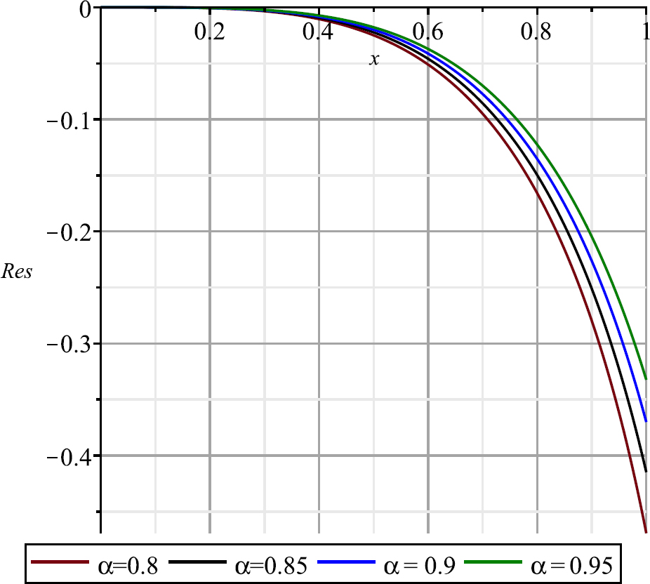
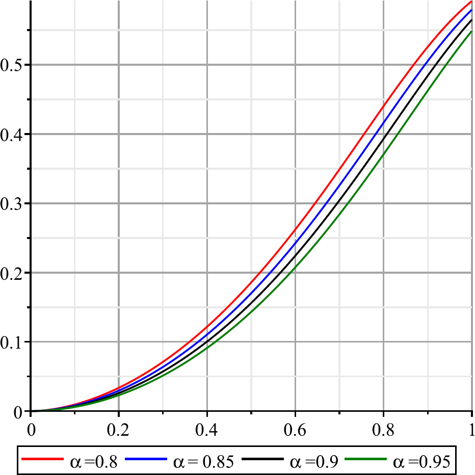
The graphs of the approximation solutions of Example 1 for N = 30 and α = 0.8, 0.85, 0.9, 0.95.
3 Solving Some example of nonlinear Abel fractional differential equation of the first kind
In this section, we apply the proposed method which is described in section 2.2, to solve some examples of nonlinear Abel fractional differential equation of the first kind (1). All examples that are chosen to solve in this section have not analytical and semi–analytical solution.
In the all of the following examples, we use the roots of shifted Chebyshev polynomials as the collocation points, the initial guess of Newton–Krylov method is vector [1, 1, ..., 1]T and numbers of Newton–Krylov iterations maximum is 10.
Now, we use the generalized minimum residual method to solve obtained linear system in each Newton iteration. We have explained this method in previous work [46, 47].
then we construct the residual function as follows:
According to collocation technique, N nonlinear equation will be obtained via (20)–(22), then by solving this nonlinear system of equations by using Newton–Krylov the approximation solution yN(x) be achieved.
Example 1.
Consider the fist example of nonlinear Abel fractional differential equation of the first kind [32, 33]:
with the initial condition:
This example has been solved by Xu and He by using the short memory principle (SMP) [33]. Also, Parand and Nikarya have solved this example by using a collocation method based on classical Bessel function [32].
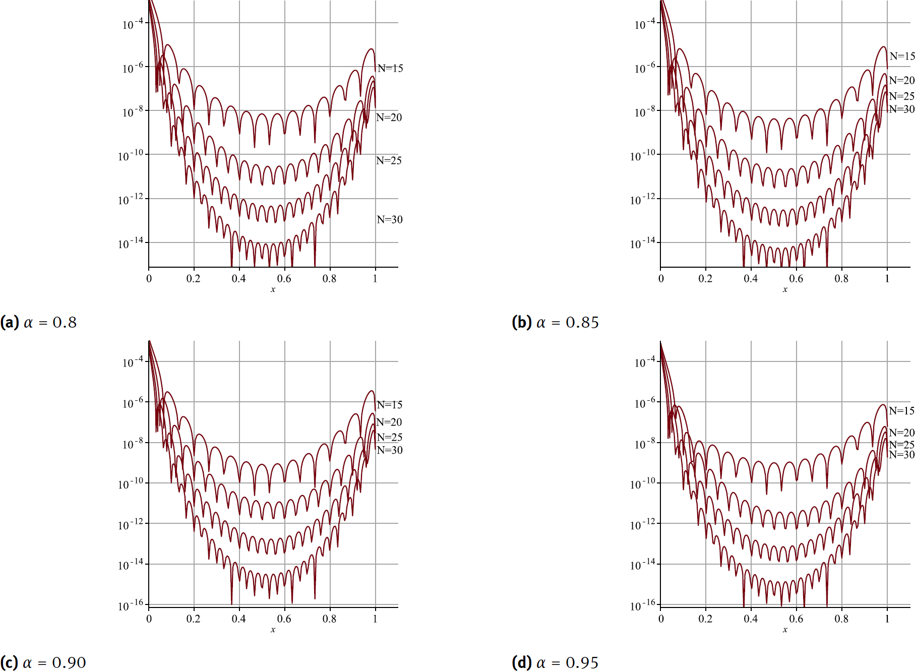
Now, we have solved this example by employing the proposed method for α = 0.8, 0.85, 0.9 and 0.95. The obtained graphs of approximation solution yN(x) of Eq. (27) are shown in Fig. 1, also in Table 1 the values of yN(x) and Res(x) is compared with results of BFC method [32] and orthogonal fractional polynomials (OFP) method[48] for several. To show the accuracy and convergency of the present method to solve this example for α = 0.8, 0.85, 0.9 and 0.95, the graphs of residual function Res(x) is presented for several N in Fig. 2, in this these graphs, we showed that, by increasing the N the residual function decreases, to show the convergence of the presented method.
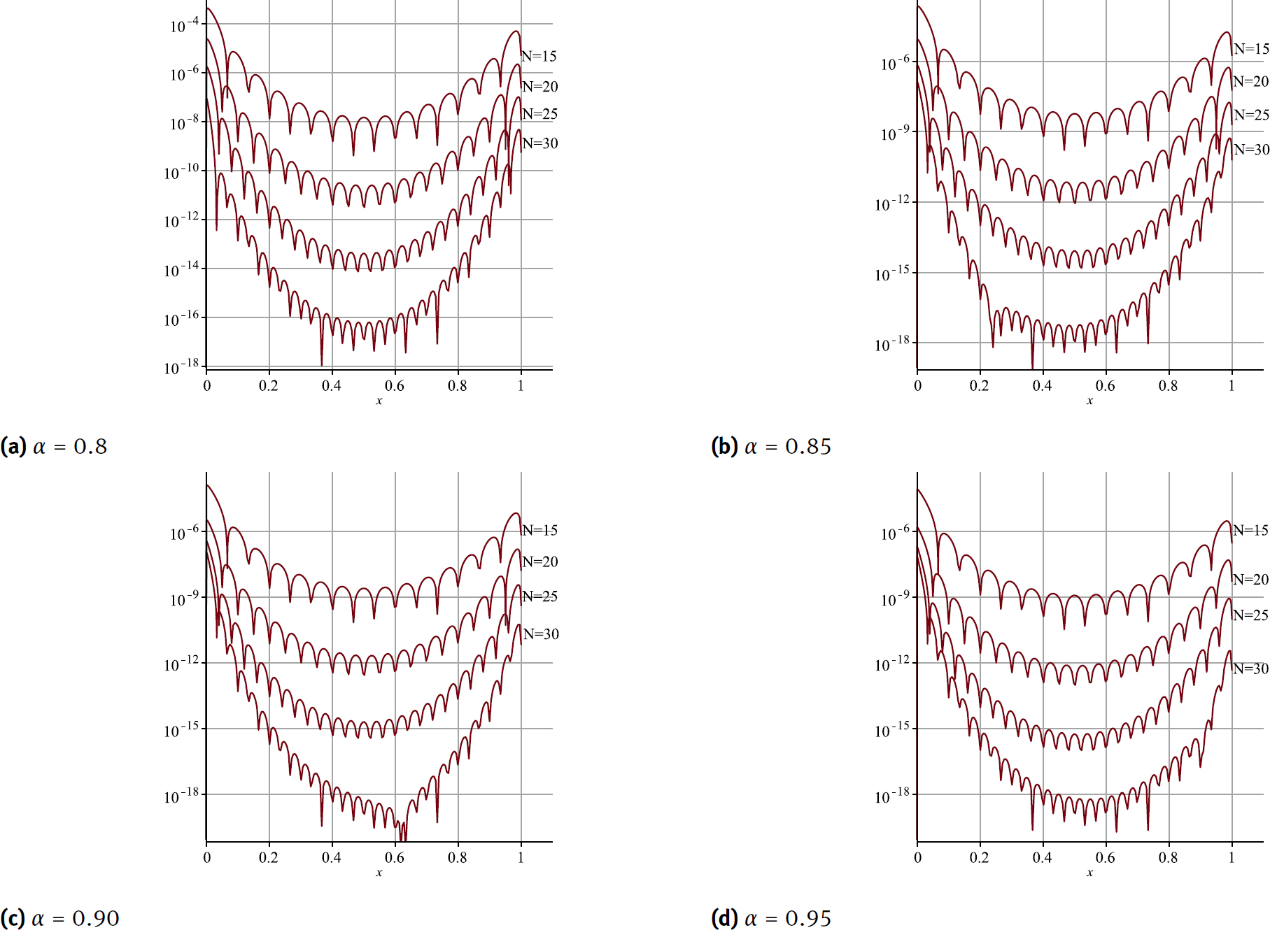
The graphs of residual function to show convergence rate of the proposed method for solving Example 1 for α = 0.8, 0.85, 0.9, 0.95 and several N.
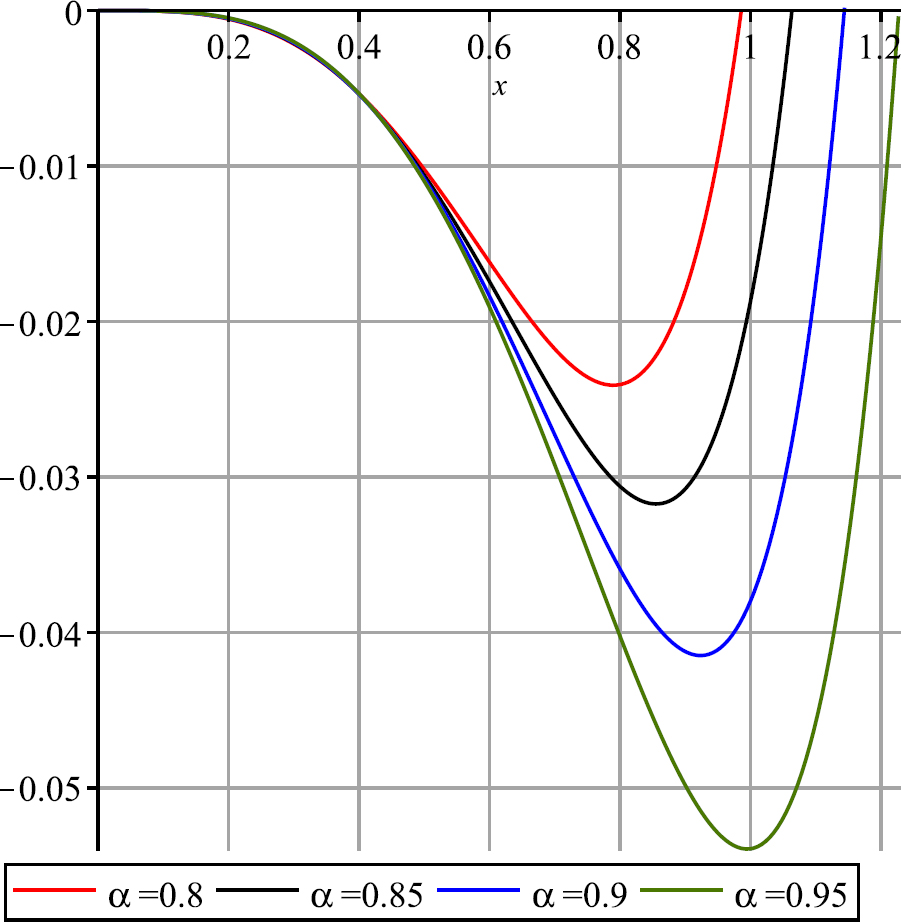
The graphs of the approximation solutions of Example 2 for α = 0.8, 0.85, 0.9, 0.95 and N = 30.
Example 2.
Consider the first kind Abel fractional differential equation:
with initial conditions:
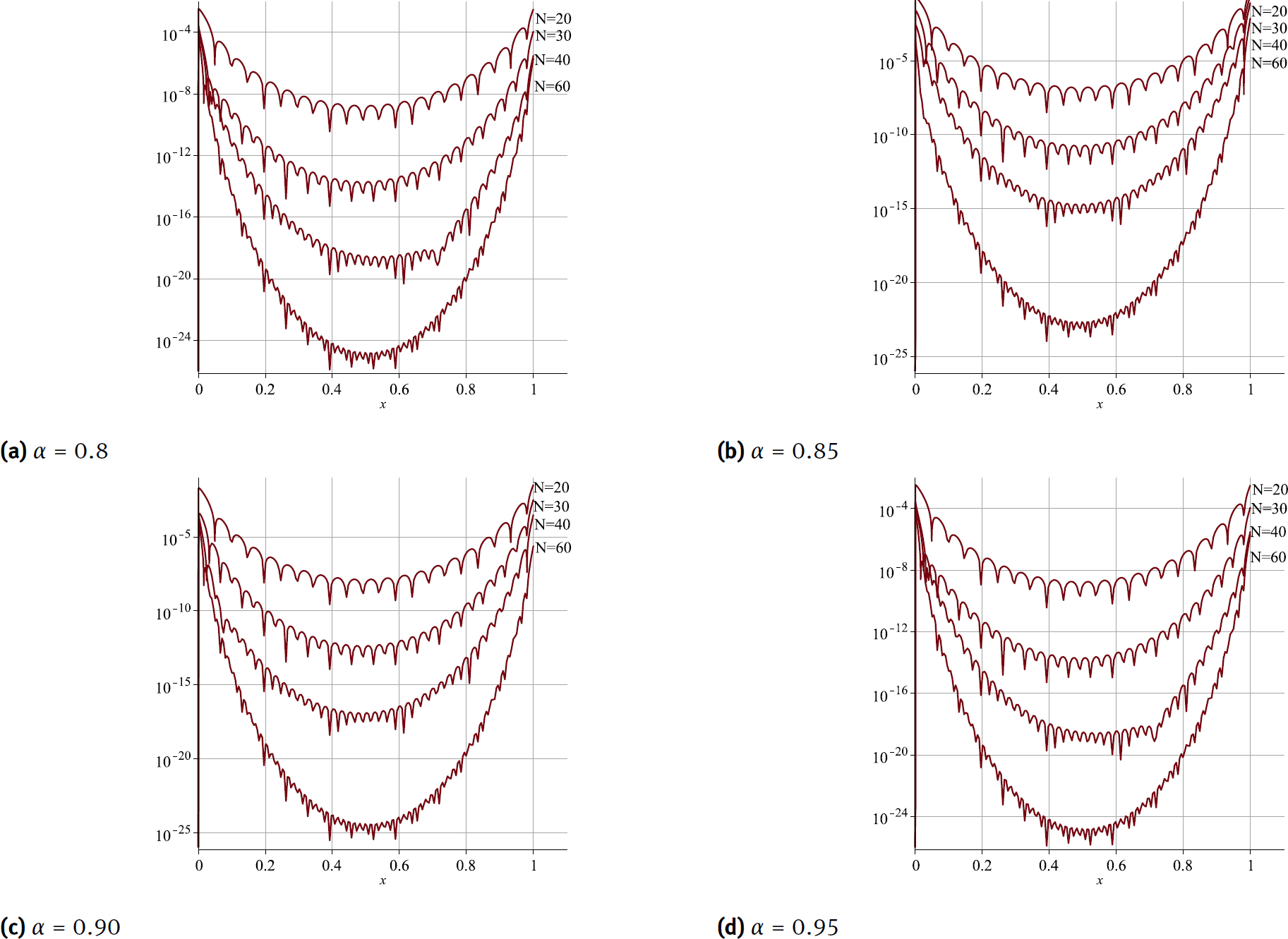
We have solved Eq. (29) by the proposed method for α = 0.8, 0.85, 0.9 and 0.95. The graphs of approximation solution yN(x) are shown in Fig. 3, in Table 2 the values of yN(x) is presented for α = 0.8, 0.85, 0.9 and 0.95. Also to show the accuracy and convergency of the present method to solve this example for α = 0.8, 0.85, 0.9 and 0.95, the graphs of residual function Res(x) is presented for several N in Fig. 4, in this these graphs, we showed that, by increasing the N the residual function decreases.
Comparison of obtained values of the proposed method and methods of [32, 48] for Example 1 for α = 0.8, 0.85, 0.9
| x | Proposed method | OFP method [48] | BFC method[32] | |||
|---|---|---|---|---|---|---|
| yN(x) | Res(x) | yN(x) | Res(x) | yN(x) | Res(x) | |
| α = 0.8 | ||||||
| 0.2 | −0.000744342596 | 5.21e − 16 | −7.443e − 4 | 4.39e − 8 | −0.000744347 | 2.34e − 7 |
| 0.4 | −0.010522091334 | 1.41e − 18 | −1.052e − 2 | 3.00e − 8 | −0.010522097 | 8.25e − 8 |
| 0.6 | −0.051085883734 | 2.12e − 18 | −5.108e − 2 | 2.06e − 8 | −0.051085888 | 4.23e − 7 |
| 0.8 | −0.165925971799 | 4.84e − 16 | −1.659e − 1 | 4.53e − 8 | −0.165925912 | 1.00e − 6 |
| 1.0 | −0.469342130398 | 5.29e − 11 | −4.693e − 1 | 7.88e − 8 | −0.469341539 | 8.71e − 5 |
| α = 0.85 | ||||||
| 0.2 | −0.000637969398 | 5.26e − 18 | ______ | ______ | −0.000637325 | 5.21e − 6 |
| 0.4 | −0.009317385395 | 1.02e − 19 | ______ | ______ | −0.009316125 | 7.16e − 6 |
| 0.6 | −0.045936456944 | 2.19e − 19 | ______ | ______ | −0.045937147 | 9.43e − 6 |
| 0.8 | −0.149705797239 | 5.53e − 17 | ______ | ______ | −0.149708698 | 5.18e − 5 |
| 1.0 | −0.414921134187 | 6.04e − 11 | ______ | ______ | −0.414919988 | 4.36e − 4 |
| α = 0.9 | ||||||
| 0.2 | −0.000546521537 | 1.41e − 17 | −5.465e − 4 | 1.66e − 09 | −0.0005465031 | 3.26e − 6 |
| 0.4 | −0.008248714922 | 3.63e − 20 | −8.248e − 3 | 1.06e − 09 | −0.0082482782 | 4.28e − 6 |
| 0.6 | −0.041322824126 | 2.82e − 21 | −4.132e − 2 | 9.61e − 10 | −0.0413235146 | 8.33e − 6 |
| 0.8 | −0.135349790084 | 4.30e − 18 | −1.353e − 1 | 9.78e − 10 | −0.1353508143 | 2.90e − 5 |
| 1.0 | −0.370165019409 | 6.84e − 12 | −3.701e − 1 | 1.49e − 09 | −0.3701646146 | 2.31e − 4 |
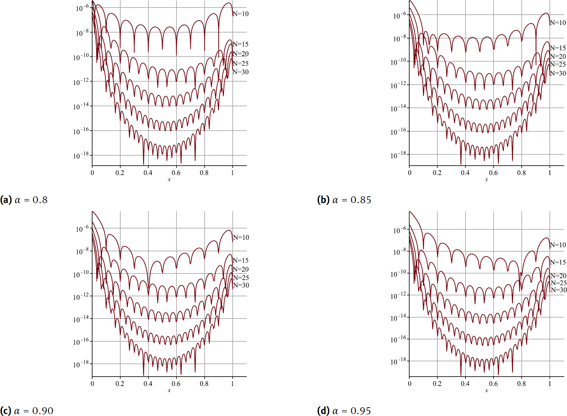
The graphs of residual function to show convergence rate of the proposed method for solving Example. 2 for α = 0.8, 0.85, 0.9, 0.95 and several N.
The values of approximation solution yN(x) of Example 2 for α = 0.8, 0.85, 0.9, 0.95 and N = 30
| x | α = 0.8 | α = 0.85 | α = 0.9 | α = 0.95 |
|---|---|---|---|---|
| 0.2 | −0.0005475041 | −0.0005222619 | −0.0004968084 | −0.0004718497 |
| 0.4 | −0.0053435740 | −0.0053795562 | −0.0053722684 | −0.0053332339 |
| 0.6 | −0.0161724534 | −0.0174150949 | −0.0183578125 | −0.0190602822 |
| 0.8 | −0.0240508103 | −0.0305890412 | −0.0359020939 | −0.0402140291 |
| 1.0 | 0.00457208778 | −0.0187336581 | −0.0379851769 | −0.0538981175 |
The values of approximate solution yN(x) of Example 3 for α = 0.8, 0.85, 0.9, 0.95 and N = 30
| x | α = 0.8 | α = 0.85 | α = 0.9 | α = 0.95 |
|---|---|---|---|---|
| 0.2 | 0.03363616357 | 0.02961943104 | 0.02608193866 | 0.022960828432 |
| 0.4 | 0.12181916687 | 0.11053132512 | 0.10037152807 | 0.09118563054 |
| 0.6 | 0.26234938310 | 0.24253149973 | 0.22437891679 | 0.20768345736 |
| 0.8 | 0.44042831745 | 0.41646752645 | 0.39326700741 | 0.37093250960 |
| 1 | 0.59212471706 | 0.57961602578 | 0.56516743215 | 0.54897123418 |
The values of approximate solution yN(x) of Example 4 for α = 0.85, 0.9, 0.95, N = 30 and α = 0.8, N = 120
| x | α = 0.8 | α = 0.85 | α = 0.9 | α = 0.95 |
|---|---|---|---|---|
| 0.1 | 0.0096441004 | 0.0082085561 | 0.0069957467 | 0.0059478742 |
| 0.3 | 0.0757064787 | 0.0674889644 | 0.0602060179 | 0.0537146181 |
| 0.5 | 0.2157562378 | 0.1950112085 | 0.1766105697 | 0.1601707949 |
| 0.7 | 0.4861687659 | 0.4365854896 | 0.3945279816 | 0.3581641713 |
| 0.9 | 1.2377342889 | 1.0106236135 | 0.8650944099 | 0.7594334013 |
The graphs of the approximation solutions of Example 3 for N = 30 and α = 0.8, 0.85, 0.9, 0.95 and N = 30.
Example 3.
Consider the fractional differential equation:
with conditions:
We have solved Eq. (31) by the proposed method for α = 0.8, 0.85, 0.9 and 0.95. The graphs of obtained approximation solution yN(x) are shown in Fig. 5. Table 3 shows the values of yN(x) for α = 0.8, 0.85, 0.9 and 0.95. Also to show the accuracy and convergency of the present method to solve this example for α = 0.8, 0.85, 0.9 and 0.95, the graphs of residual function Res(x) is presented for several N in Fig. 6, in this these graphs, we showed that, by increasing the N the residual function decreases.
Example 4.
Consider the fractional differential equation:
with the initial condition:
This example has not the exact or analytical solution, too. This example has been solved by Xu and He by using the short memory principle (SMP) [33].
We have solved Eq. (33) by the proposed method for α = 0.8, 0.85, 0.9 and 0.95. The graphs of the obtained approximation solution yN(x) are shown in Fig. 7. Table 4 shows the values of yN(x) for α = 0.8, 0.85, 0.9 and 0.95. Also to show the accuracy and convergency of the present method to solve this example for α = 0.8, 0.85, 0.9 and 0.95, the graphs of residual function Res(x) is presented for several N in Fig. 8, in this these graphs, we showed that, by increasing the N the residual function decreases.
The graphs of residual function to show convergence rate of the proposed method for solving Example 3 for α = 0.8, 0.85, 0.9, 0.95 and several N

The graphs of the approximation solutions of Example 4 for α = 0.8, 0.85, 0.9, 95 and N = 30.
4 Conclusion
The fractional calculus and fractional differential equations have found application in different sciences. But real and practical FDEs often have not exact or analytical solution, therefore, numerical solving of the fractional differential equations have become an attractive field of applied mathematics and computer science. In this article, we have introduced a new and high accurate numerical method based on generalized Bessel function (GBF) and collocation method to solve Abel fractional differential equation of the first kind. Also, in this paper, we have introduced an explicit formula to calculate Riemann–Liouville fractional derivative and integral of GBF, this formula causes the calculations be easier and faster. In the proposed method to solve obtained nonlinear algebraic systems, we use Newton–Krylov sub-space method. In this paper, we have solved the nonlinear Abel FDE of the first kind, that has not the exact or analytical solution. In this paper, we show the applicability and reliability of the proposed method to solve nonlinear FDEs.
The graphs of residual function to show convergence rate of the proposed method for solving Example 4 for α = 0.8, 0.85, 0.9, 0.95 and several N
Acknowledgement
The corresponding author would like to thank Shahid Beheshti University for the awarded grant.
References
[1] J. T. Machado, V. Kiryakova, F. Mainardi, Recent history of fractional calculus, Commun. Nonlinear Sci. Numer. Simul. 3 (2011) 1140–1753.10.1016/j.cnsns.2010.05.027Search in Google Scholar
[2] K. Oldham, Fractional differential equations in electrochemistry, Adv. Eng. Soft. 41 (2010) 9–17.10.1016/j.advengsoft.2008.12.012Search in Google Scholar
[3] R. Hilfer, Applications of fractional calculus in physics, World Scientific Publishing Company, Singapore, 2000.10.1142/3779Search in Google Scholar
[4] K. Diethelm, The Analysis of Fractional Differential Equations, Springer-Verlag, Berlin Heidelberg, 2010.10.1007/978-3-642-14574-2Search in Google Scholar
[5] L. Suarez, A. Shokooh, An eigenvector expansion method for the solution of motion containing fractional derivatives, J. Appl. Mech. 64 (1997) 629–675.10.1115/1.2788939Search in Google Scholar
[6] Z. Odibat, S. Momani, Numerical methods for nonlinear partial differential equations of fractional order, Appl. Math. Model. 32 (2008) 28–39.10.1016/j.apm.2006.10.025Search in Google Scholar
[7] S. Momani, R. Qaralleh, Numerical approximations and Padé approximats for a fractional population growth model, Appl. Math. Model. 31 (2007) 1907–1914.10.1016/j.apm.2006.06.015Search in Google Scholar
[8] Y. Wang, Q. Fan, The second kind Chebyshev wavelet method for solving fractional differential equations, Appl. Math. Comput. 218 (2011) 8592–8601.10.1016/j.amc.2012.02.022Search in Google Scholar
[9] M. Rehman, R. A.Khan, The Legendre wavelet method for solving fractional differential equations, Commun. Nonlinear Sci. Numer. Simul. 16 (2011) 4163–4173.10.1016/j.cnsns.2011.01.014Search in Google Scholar
[10] A. Saadatmandi, M. Dehghan, A new operational matrix for solving fractional-order differential equations, Comp. Math. Appl. 59 (2010) 1326–1336.10.1016/j.camwa.2009.07.006Search in Google Scholar
[11] M. Alipour, H. Agahi, New computational techniques for solving nonlinear problems using g-fractional differential operator, J. Comput. Appl. Math. 330 (2018) 70 – 74.10.1016/j.cam.2017.08.004Search in Google Scholar
[12] Y. Ordokhani, P. Rahimkhani, A numerical technique for solving fractional variational problems by müntz–legendre polynomials, J. Appl. Math. Comput. 58 (2018) 75–94.10.1007/s12190-017-1134-zSearch in Google Scholar
[13] M. Xu, J. Niu, Y. Lin, An e˛cient method for fractional nonlinear differential equations by quasi-Newton’s method and simplified reproducing kernel method, Math. Methods Appl. Sci. 41 (2017) 5–14.10.1002/mma.4590Search in Google Scholar
[14] E. Doha, A. Bhrawy, S. Ezz-Eldien, E˛cient Chebyshev spectral methods for solving multi-term fractional orders differential equations, Appl. Math. Model. 36 (2011) 5662–5672.10.1016/j.apm.2011.05.011Search in Google Scholar
[15] L. Pezza, F. Pitolli, A multiscale collocation method for fractional differential problems, Math. Comput. Simul 147 (2017) 210–219.10.1016/j.matcom.2017.07.005Search in Google Scholar
[16] S. Esmaeili, M. Shamsi, A pseudo-spectral scheme for the approximate solution of a family of fractional differential equations, Commun. Nonlinear Sci. Numer. Simul. 16 (2011) 3646– 3654.10.1016/j.cnsns.2010.12.008Search in Google Scholar
[17] A. Pedas, E. Tamme, On the convergence of spline collocation methods for solving fractional differential equations, J. Comput. Appl. Math 235 (2011) 3502–3514.10.1016/j.cam.2010.10.054Search in Google Scholar
[18] A. Saadatmandi, M. Dehghan, A Legendre collocation method for fractional integro-differential equations, J. Vibr. Contr. 17 (2011) 2050–2058.10.1177/1077546310395977Search in Google Scholar
[19] M. Delkhosh, Introduction of derivatives and integrals of fractional order and its applications, Appl. Math. Phys. 1 (2013) 103–119.Search in Google Scholar
[20] M. Jleli, M. Kirane, B. Samet, A numerical approach based on ln-shifted Legendre polynomials for solving a fractional model of pollution, Math. Methods Appl. Sci. 40 (2017) 7356–7367.10.1002/mma.4534Search in Google Scholar
[21] A. Lotfi, S. A. Yousefi, A numerical technique for solving a class of fractional variational problems, J. Comput. Appl. Math. 237 (2013) 633–643.10.1016/j.cam.2012.08.005Search in Google Scholar
[22] R. Caponetto, S. Fazzino, A semi-analytical method for the computation of the Lyapunov exponents of fractional-order systems, Commun. Nonlinear Sci. Numer. Simul. 18 (2013) 22–27.10.1016/j.cnsns.2012.06.013Search in Google Scholar
[23] H. Khosravian-Arab, M. Dehghan, M. R. Eslahchi, Generalized Bessel functions: Theory and their applications, Math. Methods Appl. Sci. 40 (2017) 6389–6410.10.1002/mma.4463Search in Google Scholar
[24] G. Wang, Twin iterative positive solutions of fractional qdifference Schrodinger equations, Appl. Math. Lett. 76 (2018) 103 – 109.10.1016/j.aml.2017.08.008Search in Google Scholar
[25] S. Ezz-Eldien, E. Doha, A. Bhrawy, A. El-Kalaawy, J. Machado, A new operational approach for solving fractional variational problems depending on indefinite integrals, Commun. Nonlinear Sci. Numer. Simul. 57 (2018) 246 – 263.10.1016/j.cnsns.2017.08.026Search in Google Scholar
[26] K. Sayevand, K. Pichaghchi, E˛cient algorithms for analyzing the singularly perturbed boundary value problems of fractional order, Commun. Nonlinear Sci. Numer. Simul. 57 (2018) 136 – 168.10.1016/j.cnsns.2017.09.012Search in Google Scholar
[27] K. Parand, M. Nikarya, J. A. Rad, F. Baharifard, A new reliable numerical algorithm based on the first kind of Bessel functions to solve Prandtl–Blasius laminar viscous flow over a semi-infinite flat plate, Zeit. Natur. A. 67 (2012) 665–673.10.5560/zna.2012-0065Search in Google Scholar
[28] K. Parand, S. Latifi, M. Delkhosh, M. Moayeri, Generalized Lagrangian Jacobi Gauss collocation method for solving unsteady isothermal gas through a micro-nano porous medium, Eur. Phys. J. Plus 133 (2018) 28.10.1140/epjp/i2018-11859-5Search in Google Scholar
[29] K. Parand, P. Mazaheri, M. Delkhosh, A. Ghaderi, New numerical solutions for solving Kidder equation by using the rational Jacobi functions, SeMA J. 74 (2017) 569–583.10.1007/s40324-016-0103-zSearch in Google Scholar
[30] S. Yuzbasi, M. Sezer, An improved Bessel collocation method with a residual error function to solve a class of Lane-Emden differential equations, Math. Comput. Model 57 (2013) 1298– 1311.10.1016/j.mcm.2012.10.032Search in Google Scholar
[31] S. Yuzbasi, Numerical solution of the Bagley-Torvik equation by the Bessel collocation method, Math. Methods Appl. Sci. 36 (2013) 300–312.10.1002/mma.2588Search in Google Scholar
[32] K. Parand, M. Nikarya, Application of Bessel functions for solving differential and integro-differential equations of the fractional order, Appl. Math. Model. 38 (2014) 4137–4147.10.1016/j.apm.2014.02.001Search in Google Scholar
[33] Y. Xu, Z. He., The short memory principle for solving Abel differential equation of fractional order, Comput. Math. Appl. 64 (2011) 4796–4805.10.1016/j.camwa.2011.10.071Search in Google Scholar
[34] J. Gine, X. Santallusia, Abel differential equations admitting a certain first integral, J. Math. Anal. Appl. 370 (2010) 187–199.10.1016/j.jmaa.2010.04.046Search in Google Scholar
[35] M. Markakis, Closed-form solutions of certain Abel equations of the first kind, Appl. Math. Lett. 22 (2009) 1401 – 1405.10.1016/j.aml.2009.03.013Search in Google Scholar
[36] T. Harko, M. K. Mak, Exact travelling wave solutions of nonlinear reaction-convection-diffusion equations, an Abel equation based approach, J. Math. Phys. 56 (11) (2015) 111501– 111525.10.1063/1.4935299Search in Google Scholar
[37] F. Schwarz, Symmetry analysis of Abel’s equation, Stud. Appl. Math. 100 (1998) 269–294.10.1111/1467-9590.00078Search in Google Scholar
[38] R. A. Adams, Sobolev Spaces, Academic Press, New York, 1975.Search in Google Scholar
[39] W. W. Bell, Special Functions For Scientists And Engineers, Published simultaneously in Canada by D. Van Nostrand Company, (Canada), Ltd, 1967.Search in Google Scholar
[40] B. Y. Guo, Spectral methods and their applications, World Scientific, Shelton Street, Covent Garden, London WC2H 9HE, 1998.Search in Google Scholar
[41] J. Shen, T. Tang, L. L. Wang, Spectral Methods Algorithms, Analysics And Applicattions, first edition, Springer, 2001.Search in Google Scholar
[42] K. Parand, M. Delkhosh, Accurate solution of the Thomas– Fermi equation using the fractional order of rational Chebyshev functions, J. Comput. Appl. Math. 317 (2017) 624 – 642.10.1016/j.cam.2016.11.035Search in Google Scholar
[43] K. Parand, M. Delkhosh, An e˛cient numerical solution of nonlinear Hunter–Saxton equation, Commun. Theor. Phys. 67 (2017) 483.10.1088/0253-6102/67/5/483Search in Google Scholar
[44] J. P. Boyd, Chebyshev and Fourier spectral methods. 2nd ed, New York Dover, 2000.Search in Google Scholar
[45] K. Parand, J. A. Rad, M. Nikarya, A new numerical algorithm based on the first kind of modified Bessel function to solve population growth in a closed system, Int. J. Comput. Math. 91 (2014) 1239–1254.10.1080/00207160.2013.829917Search in Google Scholar
[46] K. Parand, M. Nikarya, A numerical method to solve the 1D and the 2D reaction diffusion equation based on Bessel functions and jacobian free Newton–Krylov subspace methods, Eur. Phys. J. Plus 132 (2017) 496–514.10.1140/epjp/i2017-11787-xSearch in Google Scholar
[47] K. Parand, M. Nikarya, A novel method to solve nonlinear Klein-Gordon equation arising in quantum field theory based on Bessel functions and Jacobian free Newton-Krylov subspace methods, Commun. Theor. Phys. 69 (2018) 637.10.1088/0253-6102/69/6/637Search in Google Scholar
[48] K. Parand, M. Delkhosh, M. Nikarya, Novel orthogonal functions for solving differential equations of arbitrary order, Tbilisi Mathematical Journal 10 (2017) 31 – 55.10.1515/tmj-2017-0004Search in Google Scholar
© 2019 K. Parand and M. Nikarya, published by De Gruyter.
This work is licensed under the Creative Commons Attribution 4.0 Public License.
Articles in the same Issue
- Chebyshev Operational Matrix Method for Lane-Emden Problem
- Concentrating solar power tower technology: present status and outlook
- Control of separately excited DC motor with series multi-cells chopper using PI - Petri nets controller
- Effect of boundary roughness on nonlinear saturation of Rayleigh-Taylor instability in couple-stress fluid
- Effect of Heterogeneity on Imbibition Phenomena in Fluid Flow through Porous Media with Different Porous Materials
- Electro-osmotic flow of a third-grade fluid past a channel having stretching walls
- Heat transfer effect on MHD flow of a micropolar fluid through porous medium with uniform heat source and radiation
- Local convergence for an eighth order method for solving equations and systems of equations
- Numerical techniques for behavior of incompressible flow in steady two-dimensional motion due to a linearly stretching of porous sheet based on radial basis functions
- Influence of Non-linear Boussinesq Approximation on Natural Convective Flow of a Power-Law Fluid along an Inclined Plate under Convective Thermal Boundary Condition
- A reliable analytical approach for a fractional model of advection-dispersion equation
- Mass transfer around a slender drop in a nonlinear extensional flow
- Hydromagnetic Flow of Heat and Mass Transfer in a Nano Williamson Fluid Past a Vertical Plate With Thermal and Momentum Slip Effects: Numerical Study
- A Study on Convective-Radial Fins with Temperature-dependent Thermal Conductivity and Internal Heat Generation
- An effective technique for the conformable space-time fractional EW and modified EW equations
- Fractional variational iteration method for solving time-fractional Newell-Whitehead-Segel equation
- New exact and numerical solutions for the effect of suction or injection on flow of nanofluids past a stretching sheet
- Numerical investigation of MHD stagnation-point flow and heat transfer of sodium alginate non-Newtonian nanofluid
- A New Finance Chaotic System, its Electronic Circuit Realization, Passivity based Synchronization and an Application to Voice Encryption
- Analysis of Heat Transfer and Lifting Force in a Ferro-Nanofluid Based Porous Inclined Slider Bearing with Slip Conditions
- Application of QLM-Rational Legendre collocation method towards Eyring-Powell fluid model
- Hyperbolic rational solutions to a variety of conformable fractional Boussinesq-Like equations
- MHD nonaligned stagnation point flow of second grade fluid towards a porous rotating disk
- Nonlinear Dynamic Response of an Axially Functionally Graded (AFG) Beam Resting on Nonlinear Elastic Foundation Subjected to Moving Load
- Swirling flow of couple stress fluid due to a rotating disk
- MHD stagnation point slip flow due to a non-linearly moving surface with effect of non-uniform heat source
- Effect of aligned magnetic field on Casson fluid flow over a stretched surface of non-uniform thickness
- Nonhomogeneous porosity and thermal diffusivity effects on stability and instability of double-diffusive convection in a porous medium layer: Brinkman Model
- Magnetohydrodynamic(MHD) Boundary Layer Flow of Eyring-Powell Nanofluid Past Stretching Cylinder With Cattaneo-Christov Heat Flux Model
- On the connection coefficients and recurrence relations arising from expansions in series of modified generalized Laguerre polynomials: Applications on a semi-infinite domain
- An adaptive mesh method for time dependent singularly perturbed differential-difference equations
- On stretched magnetic flow of Carreau nanofluid with slip effects and nonlinear thermal radiation
- Rational exponential solutions of conformable space-time fractional equal-width equations
- Simultaneous impacts of Joule heating and variable heat source/sink on MHD 3D flow of Carreau-nanoliquids with temperature dependent viscosity
- Effect of magnetic field on imbibition phenomenon in fluid flow through fractured porous media with different porous material
- Impact of ohmic heating on MHD mixed convection flow of Casson fluid by considering Cross diffusion effect
- Mathematical Modelling Comparison of a Reciprocating, a Szorenyi Rotary, and a Wankel Rotary Engine
- Surface roughness effect on thermohydrodynamic analysis of journal bearings lubricated with couple stress fluids
- Convective conditions and dissipation on Tangent Hyperbolic fluid over a chemically heating exponentially porous sheet
- Unsteady Carreau-Casson fluids over a radiated shrinking sheet in a suspension of dust and graphene nanoparticles with non-Fourier heat flux
- An efficient numerical algorithm for solving system of Lane–Emden type equations arising in engineering
- New numerical method based on Generalized Bessel function to solve nonlinear Abel fractional differential equation of the first kind
- Numerical Study of Viscoelastic Micropolar Heat Transfer from a Vertical Cone for Thermal Polymer Coating
- Analysis of Bifurcation and Chaos of the Size-dependent Micro–plate Considering Damage
- Non-Similar Comutational Solutions for Double-Diffusive MHD Transport Phenomena for Non-Newtnian Nanofluid From a Horizontal Circular Cylinder
- Mathematical model on distributed denial of service attack through Internet of things in a network
- Postbuckling behavior of functionally graded CNT-reinforced nanocomposite plate with interphase effect
- Study of Weakly nonlinear Mass transport in Newtonian Fluid with Applied Magnetic Field under Concentration/Gravity modulation
- MHD slip flow of chemically reacting UCM fluid through a dilating channel with heat source/sink
- A Study on Non-Newtonian Transport Phenomena in Mhd Fluid Flow From a Vertical Cone With Navier Slip and Convective Heating
- Penetrative convection in a fluid saturated Darcy-Brinkman porous media with LTNE via internal heat source
- Traveling wave solutions for (3+1) dimensional conformable fractional Zakharov-Kuznetsov equation with power law nonlinearity
- Semitrailer Steering Control for Improved Articulated Vehicle Manoeuvrability and Stability
- Thermomechanical nonlinear stability of pressure-loaded CNT-reinforced composite doubly curved panels resting on elastic foundations
- Combination synchronization of fractional order n-chaotic systems using active backstepping design
- Vision-Based CubeSat Closed-Loop Formation Control in Close Proximities
- Effect of endoscope on the peristaltic transport of a couple stress fluid with heat transfer: Application to biomedicine
- Unsteady MHD Non-Newtonian Heat Transfer Nanofluids with Entropy Generation Analysis
- Mathematical Modelling of Hydromagnetic Casson non-Newtonian Nanofluid Convection Slip Flow from an Isothermal Sphere
- Influence of Joule Heating and Non-Linear Radiation on MHD 3D Dissipating Flow of Casson Nanofluid past a Non-Linear Stretching Sheet
- Radiative Flow of Third Grade Non-Newtonian Fluid From A Horizontal Circular Cylinder
- Application of Bessel functions and Jacobian free Newton method to solve time-fractional Burger equation
- A reliable algorithm for time-fractional Navier-Stokes equations via Laplace transform
- A multiple-step adaptive pseudospectral method for solving multi-order fractional differential equations
- A reliable numerical algorithm for a fractional model of Fitzhugh-Nagumo equation arising in the transmission of nerve impulses
- The expa function method and the conformable time-fractional KdV equations
- Comment on the paper: “Thermal radiation and chemical reaction effects on boundary layer slip flow and melting heat transfer of nanofluid induced by a nonlinear stretching sheet, M.R. Krishnamurthy, B.J. Gireesha, B.C. Prasannakumara, and Rama Subba Reddy Gorla, Nonlinear Engineering 2016, 5(3), 147-159”
- Three-Dimensional Boundary layer Flow and Heat Transfer of a Fluid Particle Suspension over a Stretching Sheet Embedded in a Porous Medium
- MHD three dimensional flow of Oldroyd-B nanofluid over a bidirectional stretching sheet: DTM-Padé Solution
- MHD Convection Fluid and Heat Transfer in an Inclined Micro-Porous-Channel