Inhomogeneous broadening in the time domain
-
Ludmila J. Prokopeva
 and
Alexander V. Kildishev
and
Alexander V. Kildishev


Abstract
Forty-five years after the initial attempts – first by Efimov–Khitrov in 1979, then by Brendel–Bormann in 1992 – we present a comprehensive, causal, and physically consistent framework for modeling the dielectric function with inhomogeneous (non-Lorentzian) broadening, where scattering becomes frequency- or time-dependent. This theoretical framework is based on spectral diffusion, described in the frequency domain by a complex probability density function and in the time domain by a matching characteristic function. The proposed approach accurately models the lineshapes resulting from multiple broadening mechanisms and enables the retrieval of intrinsic homogeneous linewidths as well as inhomogeneous disorder-controlled material dispersion features. To implement the new general dispersion function in time-domain Maxwell solvers, we have designed a constrained minimax-based semi-analytical approximation method (MiMOSA) that generates the shortest possible numerical stencils for a given approximation error. Application examples of exact and approximate MiMOSA models include the Gauss–Lorentz oscillator, Gauss–Debye relaxation, and Gauss–Drude conductivity. Although this study primarily focuses on the optical domain, the resulting models, which account for the Doppler shift, are equally applicable to other wave propagation phenomena in disordered dispersive media in a broad range of areas, including acoustics, magnonics, astrophysics, seismology, plasma, and quantum technologies.
1 Introduction
The fundamental understanding and predictive modeling of the broadening of the spectral line in optical systems require careful consideration of homogeneous and inhomogeneous mechanisms. These processes play crucial roles in determining the optical response of materials and are essential for understanding spectroscopic measurements and laser physics [1].
Homogeneous Broadening (HB). HB represents broadening mechanisms that affect all atoms or molecules in a system identically, arising primarily from the finite lifetime of excited states through the energy-time uncertainty principle, ΔEΔt ∼ ℏ, [2]. In the statistical sense, the HB process is intimately connected to the Cauchy distribution (also referred to as Cauchy–Lorentz or Lorentz, Eq. (12)). This distribution arises naturally from the solution of the quantum-mechanical equation of motion for a damped oscillator, which models the atomic transition. The Cauchy distribution’s “heavy tails” (with slower decay than a Gaussian) reflect the fundamental nature of the uncertainty principle. The Cauchy distribution belongs to the class of stable distributions. Thus, in the presence of several HB mechanisms associated with the same transition frequency Ω, a sum of coherent Cauchy-distributed variates ∑ i Cauchy(Ω, γ i ) matches distribution of Cauchy(Ω, ∑ i γ i ), preserving the location parameter Ω, as depicted in Figure 1(a). The resulting absorption spectrum follows a Lorentzian lineshape 1/(1 + x 2) with a resonant frequency Ω and a half-width-at-half-maximum (HWHM) given by γ = ∑ i γ i .
![Figure 1:
Broadening mechanisms in ordered and disordered media. (a) Ordered materials have a structured molecular or engineered arrangement, with a Lorentzian lineshape of absorption ɛ″(ω) [3]; (b) disordered materials, with lineshapes combining homogeneous (Lorentzian, γ) and inhomogeneous (e.g., Gaussian, σ) broadening, are largely inaccessible to time-domain nanophotonics due to the lack of efficient and physics-consistent models; examples: random metasurfaces, semi-continuous metal films, perovskites [4], MXenes [5], defects in oxides [6]. The peak decompositions are illustrative approximations rather than mathematically precise representations.](/document/doi/10.1515/nanoph-2025-0044/asset/graphic/j_nanoph-2025-0044_fig_001.jpg)
Broadening mechanisms in ordered and disordered media. (a) Ordered materials have a structured molecular or engineered arrangement, with a Lorentzian lineshape of absorption ɛ″(ω) [3]; (b) disordered materials, with lineshapes combining homogeneous (Lorentzian, γ) and inhomogeneous (e.g., Gaussian, σ) broadening, are largely inaccessible to time-domain nanophotonics due to the lack of efficient and physics-consistent models; examples: random metasurfaces, semi-continuous metal films, perovskites [4], MXenes [5], defects in oxides [6]. The peak decompositions are illustrative approximations rather than mathematically precise representations.
The most fundamental example of HB is a natural line broadening (γ natural) due to the finite lifetime of excited states. Additional HB mechanisms include pressure broadening (γ collision) in gases [7], where collisions interrupt the phase of atomic oscillations, and phonon scattering (γ phonon) in solids, which contributes to dephasing processes [8]. Using the stability of the Cauchy distribution, the total homogeneous linewidth is expressed as γ = γ natural + γ collision + γ phonon.
In the modeling sense, this simplest class of dispersion assumes that individual sources of electromagnetic response (e.g., electrons) follow identical equations of motion, with the total macroscopic model achieved via multiplication by the volume-averaged number of sources.
Inhomogeneous Broadening (IB). In contrast to HB, IB creates distinct subgroups of atoms or molecules with different resonant frequencies, fundamentally altering the optical response of the material system [9]. For example, in quantum dots, this phenomenon manifests itself through size distribution effects [10]. At the same time, in amorphous materials, it is caused through local structural variations modifying the electronic density of states [11], and in gas-phase systems through the IB-inducing thermal motion [12]. For example, IB plays a crucial role in modifying the optical response of quantum and nanoscale systems. In quantum cascade lasers, IB impacts emission properties, with the linewidth enhancement factor introducing phase-amplitude coupling that affects frequency comb formation [13]. At the quantum well level, studies have shown that interface roughness and well width fluctuations can lead to a significant broadening of intersubband absorption bands, with spectral hole burning experiments revealing the interplay between homogeneous and inhomogeneous contributions [14]. These IB effects have important implications for device design, as demonstrated in early work exploring intersubband scattering and coherent phenomena [15]. The fundamental understanding of IB mechanisms, presented, for example, in the work on quantum well structures [16], remains crucial to engineering and optimizing the performance of quantum and nanophotonic devices. In addition, optical materials can have intrinsic natural and fabrication defects, disorder, or amorphous structure. For example, in nanoplasmonic systems, IB arises from geometric variations in fabricated structures – even small polydispersity in parameters, such as plasmonic nanorod dimensions, can dramatically alter the optical spectra of their ensembles compared to individual elements[1] [19]. IB also occurs in natural crystals such as lithium niobate, where asymmetric infrared absorption arises from multiple anharmonic decay paths of phonon–polaritons into low-frequency phonons [20]. Finally, in photonics and plasma physics, individual carriers undergo a Doppler shift due to the Maxwellian distribution of their velocities [12]. As a result, real measured spectra deviate from the ideal Lorentzian absorption lineshape, 1/(1 + x 2), since the observed absorption peaks include two broadening mechanisms – homogeneous (γ) and inhomogeneous (σ, e.g., Gaussian), Figure 1(b). Retrieving both broadening components (γ and σ) is essential for capturing the underlying physics and tailoring the response, and requires physically consistent non-Lorentzian permittivity models.
Currently, to account for diverse IB effects with non-Lorentzian lineshapes, most ellipsometry fitting software relies on empirical frequency-domain approximations [21], [22]. Common examples include the pseudo-Voigt profile [23], which approximates the convolution of Lorentzian and Gaussian broadening functions (16b) with a weighted sum, and Kim’s model [24], [25], [26], which uses an empirical FD α-switch of the form
Modern Experimental Techniques. The comprehensive understanding, along with predictive and efficient numerical modeling of broadening mechanisms, have profound implications for ultra-fast laser physics [31], nanophotonic devices [32], and quantum technologies [33]. Recent advances in experimental techniques [34] continue to reveal new aspects of these fundamental processes and revolutionize our ability to study broadening mechanisms through the single-molecule [35], ultrafast [36] two-dimensional [37], and coherent multidimensional [38] spectroscopic techniques. These methods enable direct observation of individual quantum systems, provide temporal resolution of broadening dynamics, and separate homogeneous and inhomogeneous contributions. Novel spectroscopic methods [39] and advances in single-molecule detection [40] drive the development of new efficient numerical schemes that can further elucidate the complex interplay between diverse broadening phenomena and their role in areas ranging from plasma physics to emerging quantum technologies.
Numerical Modeling in the Time Domain (TD). The first TD models of HB dispersion were coupled with the classical finite-difference time-domain (FDTD) approximations of the Maxwell equations in the 1990s [41], [42]. Since then, multiple discretization techniques based on auxiliary differential equations (ADE) [43], [44], recursive convolution (RC) [45], [46], [47], [48], and Z-transform [49] have been developed. These methods assumed the classical Lorentz, Drude, and Debye dispersion models, where the dielectric function was given as a rational function in the FD, resulting in a set of exponential terms in the TD and ordinary differential equations with constant coefficients.
To date, efficient TD approximation schemes have been unavailable for simulations of dielectric functions that do not belong to the classical rational class. In some cases, the traditional non-Lorentzian empirical FD models are not even causal.
The present work addresses this problem for a broad class of natural and artificial materials with non-Lorentzian dispersion, where statistical averaging of individual sources results in convolved integral models. The approach begins with a causal exact description compatible with TD, where a fundamental dispersion formula is derived for an arbitrary absorption probability profile (Section 2). Section 3 expands the general formula into dispersion models for various broadening functions, yielding standard Lorentzian-type models (e.g., Lorentz, Debye, Drude) and new causal models based on Gaussian and Voigt profiles. All the models are summarized in Appendix A, Table A.
The implementation of new non-Lorentzian dispersion models in time-domain solvers (e.g., FDTD) is developed using a minimax-optimized semi-analytical approximation (MiMOSA), initially demonstrated for a causal Gaussian oscillator model [50]; here, we generalize and extend this approach to the Gauss–Lorentz, Gauss–Drude, and Gauss–Debye models (Section 3.4).
2 Methods
2.1 Probability formalism for dispersion
This section aims to formulate the material dispersion through the concept of photon absorption probabilities (or broadening functions
[3]) G
i
(x), enabling generalization of classical dielectric laws from Lorentz broadening to arbitrary distributions. We start with a representation of complex relative permittivity in the time and frequency domains, connected via the Fourier transform[4] (FT,
where, for generality, standard high-frequency permittivity (ɛ ∞) and conductivity terms (with DC electric conductivity σ e) are assumed [53].
The dispersion terms
Each PDF G
i
(x) is parameterized by the mean (μ
i
), variance
In the time domain, obtained via the inverse FT and applying the convolution theorem, Eq. (2) reads
where the symmetric broadening functions G i (x) contribute through its characteristic functions (CF) φ i (t) [54]. Standard CF properties include boundedness and zero-centered unity, |φ i (t)| ≤ 1 and φ i (0) = 1; moreover, if the PDF is symmetric, its CF is real-valued.
As a clear example, we reformulate the classical Lorentz oscillator using the proposed formalism
Here f, γ are oscillator’s strength and damping parameters, while Ω and
Substituting the general form of the unbroadened susceptibilities
where
Real and imaginary parts of susceptibility
Equation (5) represents a powerful theoretical framework that generates physically consistent permittivity models for any probability distribution with known complex PDFs
2.2 Analytical constraints
Time-domain modeling requires the dielectric function to be physically consistent, ensuring analyticity in the upper half-plane, causality, time-reversal symmetry (T-symmetry), Kramers–Kronig (KK) consistency, passivity and proper decay at infinity to satisfy the sum rule.
Causality of the total permittivity (ɛ(t) = 0, ∀t < 0) in Eq. (1a) is ensured as long as the unbroadened functions
T-symmetry and KK-consistency. The real and imaginary parts of each term in (1b) satisfy the time-reversal symmetry
For symmetric distributions G
i
(x) = G
i
(−x), convolution (2) holds these properties, provided the unbroadened functions
Sum rules. In ultrafast TD modeling, physically accurate high-frequency asymptotic behavior is important. As ω → ∞, total permittivity in Eq. (1a) should approach a free electron gas behavior: (a)
Condition (b) yields the sum rule
Condition (a) in Voigt multi-term dispersion model (16) is satisfied asymptotically, in both exact and MiMOSA models, as
Passivity of the total permittivity (ɛ″(ω) ≥ 0, ∀ω ≥ 0) is easy to ensure in the general formulation (5b) by the passivity of individual terms, provided that all phases are zero (ϕ i = 0) and the broadening functions G i (x) are bell-shaped.[7] When non-zero phases (ϕ i ≠ 0) are present, individual terms may locally exhibit gain, compensated by other terms in the total sum. A representative class of examples are MiMOSA models in Section 3.4, where coupled oscillators with conjugate poles maintain overall passivity[8] (see also Figure 5 in [50]).
3 Results
The new probability-based dispersion relation (5) extends classical (homogeneously broadened) dispersion models – Lorentz oscillator, Debye relaxation, and Drude conductivity – to the general case of Voigt (Gauss–Lorentz) broadening and other distributions. We first derive the unbroadened case (Section 3.1), then validate the fundamental formula (5) with homogeneous (Lorentz) broadening (Section 3.2) and present new models for inhomogeneous (Gaussian and Voigt) broadening in Section 3.3.[9]
3.1 Zero broadening (ZB)
ZB represents an idealized scenario with infinitely narrow spectral lines (G(x) = δ(x)) and infinite transition lifetimes. In the class of rational functions, the general form of a single-term unbroadened model is derived by taking the limit γ → 0+ in the HB case (11) resulting in
with [a, ϕ, Ω] being the amplitude, phase and oscillation frequency parameters.
The ZB formula (6) is consistent with the fundamental dispersion equation (5), where a delta function distribution is used as the PDF,
and represents zero scattering γ = 0+.[10]
The phase parameter ϕ in (6) (also known as the loss angle) mixes the real and imaginary parts and allows the transition between two orthogonal cases: (ϕ = 0, Ω > 0) representing a classical oscillator and
Lossless Lorentz oscillator (ϕ = 0, Ω > 0), also called the Sellmeier model [57], has quadratically decaying real part and delta functions in absorption
Lossless Debye relaxation
Lossless Drude model
Here ω
p is a plasma frequency – a characteristic point where the lossless Drude permittivity
The delta function terms in (6b), often omitted in the literature, represent degenerate distributions of zero width and play a key role in the convolution formalism. When the ZB model (6b) is convolved with a PDF G(x), the absorption of an oscillator (ϕ = 0) is directly linked to the function G(x) as
This is why, for example, a Gaussian distribution produces a Gaussian lineshape in the absorption. In the case of relaxation/conduction, the lineshape (of
3.2 Homogeneous broadening (HB)
HB represents the natural linewidth broadening that affects all atoms or molecules equally, due to the finite lifetime τ = γ −1 of excited states (uncertainty principle [2]). The general form of single-term HB dispersion, also known as the critical point model [60], represents an arbitrary rational function[13]
The HB case (11) can be derived by either convolving (“blurring”) the ideal unbroadened susceptibility
As expected, the parameter substitutions (outlined in parenthesis) reduce the general HB formula (11) to the classical Lorentz [61], Debye [62], and Drude [59] dispersion models, as shown below.
Lorentz oscillator
Debye relaxation
Drude model
In the Drude case, convolution with unbroadened susceptibility (10b) is unphysical but valid for its unbroadened conductivity function (10a), with χ(.) restored from σ(.) afterward.12
3.3 Inhomogeneous broadening (IB)
IB arises from statistical distribution of microscopic resonant frequencies Ω affected by local environmental variations and the Doppler shift.[14] As a result, the observed spectral broadening deviates from the ideal Lorentzian lineshape to a mix of both – natural lifetime-based (HB) defined by γ and statistical (e.g., Gaussian) broadening defined by variance σ 2 (Figure 1), leading to the general Gauss–Lorentz model
where w(z) is the Faddeeva (Kramp) function [63].
The IB formula (16) is obtained as a convolution of the unbroadened response
corresponding to the time-dependent scattering γ(t) = σ 2 t/2. In the presence of multiple broadening mechanisms, the probability theory for the sum of random variables dictates that the PDFs are convolved, while their CFs are multiplied,[15] and so the IB formula (16) can also be obtained from the general formula (5) using the Gauss–Lorentz (Voigt) PDF/CF
where the scattering function has both – the constant and the linear correction terms, γ(t) = γ + σ 2 t/2.[16]
The new Voigt formula is consistent with all limiting cases: σ → 0+ gives classical Lorentzian models (11), γ → 0+ gives pure Gaussian lineshape typical for strong disorder, while σ, γ → 0+ gives the ZB case (6). These transitions are easy to see through the general formula (5) and distributions equations (7), (12), (17) and (18).[17]
As before, we simplify the general IB formula (16) for the oscillator, relaxation, and conductivity cases, specifying the corresponding parameter substitutions.
Gauss-Lorentz oscillator (ϕ = 0,
The first causal Gaussian oscillator model (Γ = 0+) was derived in 2006 [64] using a causality tip from [65]. The first attempts to formulate the Gauss–Lorentz model date back to the late 1970s [66], with a later reproduction [67] usually referred to as the Brendel-Bormann (BB)-model. Unfortunately, the non-causal BB model, incompatible with TD, remains broadly adopted by experimentalists to fit material responses to infra-red light, e.g., [68], [69], [70]. Causal corrections with logarithmic terms, rational approximations, and ongoing discussions of the physical validity of the BB model can be found in Refs. [71], [72], [73].
Our new Gauss–Lorentz (GL) model (19) fixes all the issues with the previous BB formulation [67] (see the details in Appendix B). When σ → 0+, the GL formula gives the classical Lorentz model with 1/(1 + x 2) absorption lineshape, (13). The case of Γ → 0+ gives a causal Gaussian oscillator with exp[−x 2 ln2] absorption lineshape17 [64], while the mixed case (Γ, σ > 0) yields the Voigt profile – a new causal formulation with a time-dependent scattering function γ(t) = γ + σ 2 t/2, first mentioned by Kim et al. [24], [25], and consistent with [74].
Gauss–Debye relaxation
The limits σ → 0+ and γ → 0+ give the classical Debye (14) and a new Gauss relaxation model, respectively.17
The Gauss–Debye model (20) has not been shown in the literature. Known generalizations to the Debye relaxation – the Cole–Cole, Cole–Davidson, and Havriliak–Negami models [75], [76] – remain inaccessible to efficient TD simulations, and will be addressed in future work.
Gauss-Drude model
The limits σ → 0+ and γ → 0+ give the classical Drude model (15b) and a new Gauss conductive model, respectively.17 The derivation is based on the broadening formalism (Section 2) for the conductivity function. Comparing classical Drude model (15b) to the new Gauss conductivity model (21b), we observe lineshape change and find that disordered analogue of classic conductivity
Corrections to the classical Drude model have been widely studied, including empirical frequency-domain formulations with fractional derivatives, effective mass parameter, and modified scattering functions [77]. However, the causal Gauss–Drude model introduced here has never been presented.
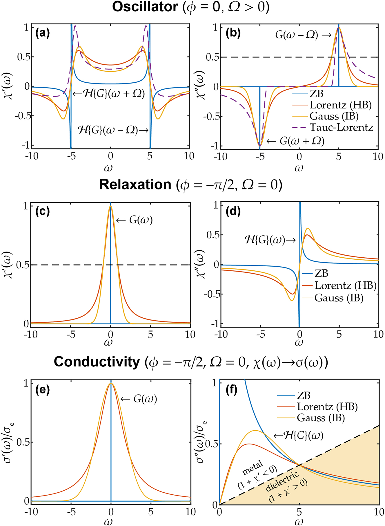
Figure 2 illustrates the final Voigt formula (16) for three cases of broadening – ZB, HB (σ = 0+) and IB (γ = 0+) for three types of dispersion: oscillator, relaxation, and conductive media. HB and IB curves are matched at the peak maximum and full-width-half-maximum (FWHM) of the real (for relaxation) or imaginary (for oscillator) parts, demonstrating the deviation of the “heavy-tail” Lorentzian lineshape
These plots effectively illustrate the physical interpretation of the complex PDF
3.4 Minimax approximation (MiMOSA)
When the broadening function G(x) is non-Lorentzian, the general dispersion formula (5) falls outside of the class of the rational functions of argument s = −ıω, and cannot be immediately translated into auxiliary differential equations, making it challenging to construct short discretization stencils and coupling to time-domain solvers, such as FDTD. The solution for efficient TD implementation of non-Lorentzian dispersion was first developed for a pure Gaussian oscillator [50], and employs minimax optimization to generate the shortest possible time stencil for a given error (MiMOSA).
Derivation of MiMOSA (Mini-max optimized semianalytical approximation) models for a general dispersion formula (5) starts with a minimax rational approximation[18] of the complex PDF
For example, for the Voigt distribution (18), the approximation coefficients [B j , C j ] are calculated for the Faddeeva function w(z), with n being the number of approximation poles, Figure 3(c),[19]
Substituting the approximation (22) into the general susceptibility formula (5) gives a set of FDTD-compatible analytically derived dispersion terms
where parameters [a j , ϕ j , Ω j , γ j ] are directly connected to the parameters of the exact single-term model [a, ϕ, Ω, γ, σ] (5) and the approximation constants [B j , C j ] in (22) as
The MiMOSA model (24)–(25) retains the single-oscillator form [78], with only its envelope modified by approximation (compare to the exact susceptibility χ(t)),
This identity arises by substituting coefficients (25) into the time-domain expression (24) and combining the conjugate pole pairs. It ensures that the model remains physically consistent, without introducing nonphysical oscillations.
Due to the equioscillation theorem [79], the minimax solution provides the shortest rational polynomial approximation (corresponding to most compact numerical stencil), with the approximation error spread evenly across the entire frequency domain. In the Voigt case
The MiMOSA models (24) fit the class of rational functions that can be coupled efficiently to the TD Maxwell’s solvers. Detailed ADE and RC numerical schemes for this class of dispersion can be found in Refs. [50], [80], [81] for second-order accurate TD solvers, and in Refs. [82], [83], [84] for higher-order schemes. We recommend using the universal compact scheme, which minimizes computational cost per dispersion term and enables easy switching between different second-order accurate ADE and RC formulations. An FDTD code implementing six such schemes is available in Ref. [50].
Compared to the approximations derived in the 1950s by reincarnating the minimax methods for rational polynomials and the more recent literature on the rational approximations to Faddeeva/Kramp/plasma dispersion function (or their real/imaginary parts) [85], [86], [87], [88], [89], [90], [91], [92], [93], [94], [95], [96], [97], [98], [99], [100], [101], [102], our MiMOSA method achieves impressive
A related computational approach has been recently proposed in Ref. [103], where an ab initio integral dispersion formulation is presented and subsequently transformed into a rational function through a quadrature approximation, thereby preserving the physical meaning of the main model parameters. However, no alternative approximation technique achieves the same minimal number of additional equations as MiMOSA for a given maximal error across the entire upper half-space.
4 Conclusions
This work advances the field of computational nanophotonics by introducing a general theoretical framework to model inhomogeneous broadening in disordered, defect-containing, and amorphous materials based on the absorption probability density functions G(x). The new formulation employs a complex absorption probability density,
Application examples of the theory include Gauss–Lorentz oscillator, Gauss–Debye relaxation, and Gauss–Drude conductivity models for the characterization and predictive modeling of inhomogeneous broadening effects in linear and nonlinear regimes and provide a critical fix to the noncausal Brendel–Bormann model (see Appendix B for comparison). The complete set of newly derived dispersion models is presented in Table A, Appendix A.
The exact generalized permittivity formulation is then used to obtain the efficient, best-possible minimax-based approximation (MiMOSA) models that enable (1) integral- and special-function-free permittivity calculation; (2) efficient FDTD implementation with a minimal set of the additional equations; and (3) ellipsometry fitting and lineshape retrieval. The MiMOSA implementation ensures efficient simulation while maintaining the desired controlled accuracy and analytical constraints.
The near-term work includes extending our approach to nonsymmetric distributions (e.g., the Fermi–Dirac distribution), and next-order corrections in the scattering function γ(t) = γ + σ 2 t/2 + ···, as well as developing the time-domain approximations to the widely used empirical non-symmetric models, including the Tauc(Cody)–Lorentz dispersion [27], [28] (Figure 2(a) and (b)). The proposed formulation for arbitrary probability density functions can become a foundational model for inhomogeneous broadening analysis. Its ability to retrieve broadening information through minimax coefficients and fitting to experimental data can provide invaluable insights into the lifetime-based width, local environments, and the nature of disorder in materials, thus improving our understanding of their fundamental properties [104].
Our approach extends naturally to anisotropic and bi-anisotropic materials involving full electromagnetic tensors, as well as to nonlinear models such as saturable Lorentz and multilevel carrier kinetics solvers, where the non-Lorentzian lineshapes can now be accurately implemented in FETD, DGTD, FVTD or FDTD solvers. Although this result focuses primarily on optical materials and nanophotonics, its implications extend broadly to wave propagation across various disciplines, including microwave electromagnetics, acoustics, electronics, magnonics, biosensing, seismology, astrophysics, and quantum information technologies, where our newly developed MiMOSA method efficiently accounts for inhomogeneous broadening in dispersive media.
Funding source: Office of Naval Research
Award Identifier / Grant number: N00014-20-S-B001
Funding source: Air Force Office of Scientific Research
Award Identifier / Grant number: FA9550-21-1-0299
-
Research funding: This work was supported by the USA ONR Award N00014-20-S-B001, the USA AFOSR Awards FA9550-21-1-0299 and FA9550-22-1-0372, and the Purdue internal SPARK program.
-
Author contributions: Both authors have accepted responsibility for the entire content of this manuscript and consented to its submission to the journal, reviewed all results, and approved its final version. LJP and AVK have made an equal contribution to the initial conception of the constrained approximants. LJP has developed exact and MiniMax-optimized permittivity models, performed their verification in FDTD. LJP and AVK prepared the manuscript.
-
Conflict of interest: Authors state no conflict of interest.
-
Data availability: All the data for the current study are available in the paper.
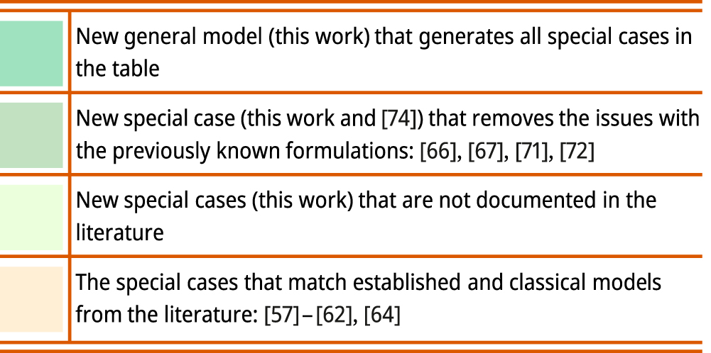
Appendix A: Table of susceptibility models with arbitrary broadening
Table A presents the Fundamental Dispersion Model (shown in the dark green cell) for any rational unbroadened dispersion function χ
0(.) broadened by an arbitrary Probability Density Function (PDF) G(x). Special cases of χ
0(.) are listed in the columns: Oscillator – difference of two complex conjugate or real poles (column 3), Relaxation – one real pole (column 4), Conductivity – difference of two real poles, one of which is zero (columns 5). Special cases of the broadening function G(x) are listed in the rows: the most general case is Any Broadening (row 2) with given Characteristic Function (CF)
 |
Susceptibility
 |
The general model is parameterized by the time-domain phase ϕ, amplitude a, resonance frequency Ω, and broadening (σ, γ) parameters, yielding simple formulas. The phase parameter ϕ allows to account for a critical point (CP) model [60], and toggles between two orthogonal cases: a relaxation (ϕ = −π/2) with one real pole s
1 = −γ, and an oscillator (ϕ = 0) with two poles s
1,2 = −γ ± ıΩ, where
Oscillator (ϕ = 0, Ω > 0) is usually defined by the natural frequency ω
0, broadening Γ, and oscillator strength f, as in
Relaxation (ϕ = −π/2, Ω = 0) corresponds to exponential decay in the time domain. Its amplitude is classically characterized by a permittivity jump Δɛ at ω = 0, with the fall rate defined by the relaxation time τ, as in
Conductivity (ϕ = −π/2, Ω = 0, χ(.) → σ(.)) is characterized by the plasma frequency ω
p and collision rate γ, as in
Appendix B: Correction to the Brendel–Bormann (BB) model
Efimov and Khitrov [66] and later Brendel and Bormann [67] postulated that the following convolution integral introduces the Voigt (Gauss–Lorentz) broadening to the classical Lorentz oscillator,
This integral can be solved in terms of Faddeeva functions, as shown in Rakić et al. [68],
While the BB model (B.2) and (B.3) can be useful in specific cases of experimental frequency-domain spectroscopy, e.g., [68], it is inherently non-causal. This drawback restricts its utility primarily to spectral fitting applications and makes it unsuitable for time-domain simulations. The properties of the BB model and possible corrections have been discussed in the literature up to today, [71], [72], [73].
In this work, we have built a physically consistent formalism for susceptibility functions broadened by any absorption probability G(x), including Voigt profile. First, we express the Lorentz oscillator with strength f, natural frequency ω 0, and (homogeneous) broadening γ = Γ/2 in the time and frequency domains,
Second, we write the Gaussian probability density function (PDF) and corresponding characteristic function (CF), both characterized by the variance σ 2,
Note that we assume zero mean (μ = 0) which keeps the resonance frequency Ω of the oscillator unshifted.
In the time domain, the Gauss–Lorentz model is a multiplication of the Lorentz oscillator (B.4) by the Gaussian CF (B.5b),
which can also be viewed as a lossless Lorentz (Sellmeier) oscillator broadened by both Cauchy and Gaussian distributions. This aligns with the general principle from probability theory: the CF of the sum of two random variables is a product of individual CFs, while the PDF of the sum is a convolution. Equation (B.6) preserves causality (note the term θ(t)) and leads to an inhomogeneous time-dependent scattering function γ(t) = γ + σ 2 t/2, where higher order correction terms are possible for other broadening functions G(x), as predicted by Kim et al. [24].
In the frequency domain, according to the convolution theorem, such multiplication corresponds to the integral
Decomposing the Lorentzian into single poles (with
making substitution x → −x in the integral for the first pole, and then (x + Ω) → x for both poles, gives the final integral (where Γ = 2γ)
and its closed-form expression in terms of the Faddeeva functions
Comparison of the GL model (B.9) with the BB model (B.3) (duplicated in (B.10) for convenience) indicates two key differences:
The resonance and natural frequencies are confused, Ω ≠ ω 0. For a mildly damped oscillator Γ ≪ ω 0 this can be a close approximation,
The BB model uses a sum of the Faddeeva functions instead of a difference. For the Lorentzians, the sum and difference are identical,
For the Voigt profile, same identity does not hold, i.e.,
Only with a negligible Gaussian width, σ ≪ Γ, the Voigt profile simplifies to a Lorentzian, and the sum can approximate the difference, which can be shown using the asymptotic formula of large arguments, w(z) ≈ ıπ −1/2 z −1. As a result, the BB model (B.3) can be useful for Gaussian broadening analysis but only becomes close to the true GL formula for feebly damped (Γ ≪ ω 0) and feebly Gaussian (σ ≪ Γ) oscillators over higher frequency ranges (ω ≫ Γ). The BB model (B.3) violates causality, which makes it unusable in time-domain simulations. Instead, the Gauss–Lorentz (GL) model (B.8) and (B.9) should be used for spectral analysis and simulations, especially in the time domain.
The new GL model is causal (χ
GL(t) = 0 ∀t < 0), has the correct symmetry
Appendix C: Equioscillation theorem and MiMOSA method
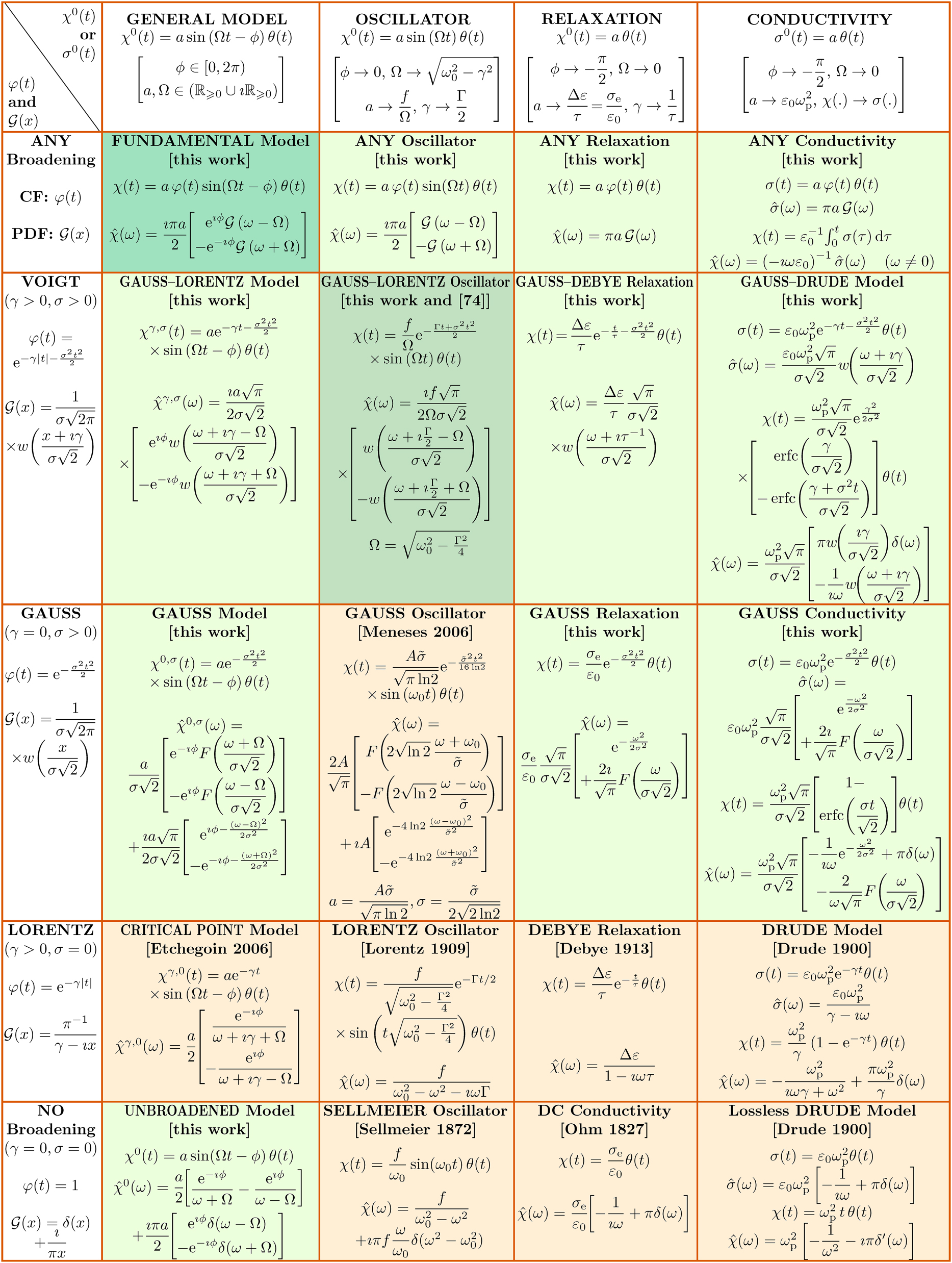
The minimax optimization technique utilized in the MiMOSA method traces its historical origins to the 19th century work of Pafnuty Tchebycheff (Chebyshev) [79]. The equioscillation theorem, also known as the Chebyshev alternation theorem, represents a fundamental principle in approximation theory. It states that, when approximating a continuous function, the optimal uniform (minimax) rational approximation of degree [M, N] exhibits a distinctive pattern: the approximation error attains its maximum absolute value at least M + N + 2 times across the interval. At these extremal points, the error alternates precisely in sign and has equal magnitude, hence the term “equioscillation”. This evenly distributed alternation of maximal error is the defining feature of the optimal solution in the minimax sense, see Figure 3(a).
![Figure 3:
Minimax approximation error. (a) Error distribution of a minimax rational approximation and a non-minimax technique (Padé, [92]) for the Dawson function F(x), both using four poles (n = 4). The minimax approximation exhibits a characteristic equioscillating error – uniformly spread with alternating sign and constant magnitude and achieving optimal accuracy across the domain. The non-minimax (Padé) method shows lower error near the origin and at infinity but significantly higher (9× larger) global maximum error than the minimax. (b) Exponential convergence of the maximum relative error with increasing number of poles (n) for both the Dawson function and the Hilbert-reconstructed Faddeeva function approximations. With each additional pole, we observe an error reduction of roughly one order of magnitude. (c) Dawson’s approximation error for coefficients (23).](/document/doi/10.1515/nanoph-2025-0044/asset/graphic/j_nanoph-2025-0044_fig_003.jpg)
Minimax approximation error. (a) Error distribution of a minimax rational approximation and a non-minimax technique (Padé, [92]) for the Dawson function F(x), both using four poles (n = 4). The minimax approximation exhibits a characteristic equioscillating error – uniformly spread with alternating sign and constant magnitude and achieving optimal accuracy across the domain. The non-minimax (Padé) method shows lower error near the origin and at infinity but significantly higher (9× larger) global maximum error than the minimax. (b) Exponential convergence of the maximum relative error with increasing number of poles (n) for both the Dawson function and the Hilbert-reconstructed Faddeeva function approximations. With each additional pole, we observe an error reduction of roughly one order of magnitude. (c) Dawson’s approximation error for coefficients (23).
The MiMOSA method starts by finding such optimal minimax rational approximation for the Hilbert transform of the probability function
Figure 3(a) illustrates the minimax concept and its advantages over non-minimax approximation methods. Shown is a relative error of the sum-rule-constrained 4-pole (n = 4) minimax rational approximation of the Dawson function (F(x) ≈ F n (x)), featuring (4n − 1) equioscillating peaks (in agreement with the alternation theorem). As a non-minimax reference, we include a 4-pole Padé approximation [92], a method that has recently gained popularity in computational modeling [100]. While the Padé approximation achieves higher precision near x = 0 and at infinity, its global maximum error in this example is 9 times larger (4.5e-3) than that of the minimax approximation (0.5e-3). In time-domain simulations, particularly those involving ultrafast phenomena, broadband accuracy is essential, making the minimax approach optimal for achieving the best overall accuracy with a fixed number of poles n.
Figure 3(b) demonstrates that the maximum relative error of the Dawson function approximation,
yields an approximation of the Faddeeva function w(z) with approximately the same maximum relative error across the entire upper half-plane,
Each additional pole reduces the error by roughly an order of magnitude, highlighting the rapid convergence of the minimax approximation.
Described properties are essential to the efficiency of MiMOSA permittivity models for the following reasons:
Optimal error distribution. MiMOSA models use minimax rational approximations to uniformly minimize error across the spectral domain, ensuring consistent broadband accuracy without localized degradation.
Minimal number of poles. High accuracy (better than 1 %) can be achieved with just 2–3 poles, significantly reducing computational cost. A smaller number of poles translates into the shortest possible time-domain stencil in the FDTD update equations, which is critical for fast and memory-efficient time-domain simulations.
Physically consistent formulation. The semi-analytical derivation with built-in constraints (e.g., causality, sum rules, Kramers–Kronig consistency) ensures that MiMOSA models maintain the structure and interpretability of a single oscillator. Unlike overfitted multi-parameter models, the compact form of MiMOSA improves fitting stability and gives physical meaning to each parameter.
Appendix D: Abbreviations and functions
PDF – Probability density function, G(x); it is nonnegative (G(x) ≥ 0) and has full probability support
Complex PDF – Probability density function with added Hilbert transform as an imaginary part,
CF – Characteristic function,
sPDF – standard PDF, g(x) = G(x;μ=0,σ
2=1) – a normalized PDF, with the argument centered and stretched such that: the mean is zero (μ = 0) and variance is one (σ = 1) leading to
Lineshape, l(x) – a normalized distribution with the argument centered and stretched and the amplitude scaled so that: the peak is centered at zero with maximum of 1 and half-width-half-maximum (HWHM) of 1. Examples: Cauchy/Lorentz
CP – Critical point model, known in the semiconductor literature [60].
FT – Fourier transform
IFT – Inverse Fourier transform
HT – Hilbert transform
IHT – Inverse Hilbert transform
TD – Time domain.
FD – Frequency domain.
ZB – Zero broadening (γ = 0+, σ = 0+).
HB – Homogeneous broadening (γ > 0, σ = 0+).
IB – Inhomogeneous broadening (γ ≥ 0, σ > 0).
The Faddeeva (or Kramp) function,
The Dawson function (or Dawson integral),
Conductivity function
The Dirac delta function, δ(x).
The Heaviside step function, θ(t).
References
[1] W. Demtroder, Laser Spectroscopy: Basic Concepts and Instrumentation, 3rd ed. Heidelberg, Germany, Springer, 2003.Search in Google Scholar
[2] V. Weisskopf and E. Wigner, “Uber die naturliche linienbreite in der strahlung des harmonischen oszillators,” (in German), Z. Phys., vol. 65, no. 1, pp. 18–29, 1930. https://doi.org/10.1007/BF01336768.Search in Google Scholar
[3] P. Spinelli, M. A. Verschuuren, and A. Polman, “Broadband omnidirectional antireflection coating based on subwavelength surface Mie resonators,” Nat. Commun., vol. 3, no. 692, pp. 1–5, 2012. https://doi.org/10.1038/ncomms1691.Search in Google Scholar PubMed PubMed Central
[4] S. N. Chowdhury, et al.., “Wide-range angle-sensitive plasmonic color printing on lossy-resonator substrates,” Adv. Optical Mater., vol. 12, no. 4, p. 2301678, 2024. https://doi.org/10.1002/adom.202301678.Search in Google Scholar
[5] J. Simon, C. Fruhling, H. Kim, Y. Gogotsi, and A. Boltasseva, “MXenes for optics and photonics,” Opt. Photonics News, vol. 34, no. 11, pp. 42–49, 2023. https://doi.org/10.1364/OPN.34.11.000042.Search in Google Scholar
[6] M. Narayanan, A. P. Shah, S. Ghosh, A. Thamizhavel, and A. Bhattacharya, “Elucidating the role of oxygen vacancies on the electrical conductivity of β-Ga2O3 single-crystals,” Appl. Phys. Lett., vol. 123, no. 17, p. 172106, 2023. https://doi.org/10.1063/5.0158279.Search in Google Scholar
[7] P. W. Anderson, “A method of synthesis of the statistical and impact theories of pressure broadening,” Phys. Rev., vol. 86, no. 5, p. 809, 1952. https://doi.org/10.1103/PhysRev.86.809.Search in Google Scholar
[8] S. Mukamel, Principles of Nonlinear Optical Spectroscopy, New York, NY, US, Oxford University Press, 1995.Search in Google Scholar
[9] A. M. Stoneham, Theory of Defects in Solids, Oxford, UK, Oxford University Press, 1975.Search in Google Scholar
[10] D. Bimberg, M. Grundmann, and N. N. Ledentsov, Quantum Dot Heterostructures, Chichester, UK, Wiley, 1999.Search in Google Scholar
[11] S. R. Elliott, Physics of Amorphous Materials, 2nd ed. Harlow, UK, Longman, 1990.Search in Google Scholar
[12] R. H. Dicke, “The effect of collisions upon the Doppler width of spectral lines,” Phys. Rev., vol. 89, no. 2, pp. 472–473, 1953. https://doi.org/10.1103/PhysRev.89.472.Search in Google Scholar
[13] M. Piccardo, et al.., “Frequency combs induced by phase turbulence,” Nature, vol. 582, no. 7812, pp. 360–364, 2020. https://doi.org/10.1038/s41586-020-2386-6.Search in Google Scholar PubMed
[14] F. Demangeot, D. Simeonov, A. Dussaigne, R. Butté, and N. Grandjean, “Homogeneous and inhomogeneous linewidth broadening of single polar GaN/AlN quantum dots,” Phys. Status Solidi C, vol. 6, no. S2, pp. S598–S601, 2009. https://doi.org/10.1002/pssc.200880971.Search in Google Scholar
[15] J. Faist, et al.., “Measurement of the intersubband scattering rate in semiconductor quantum wells by excited state differential absorption spectroscopy,” Appl. Phys. Lett., vol. 63, no. 10, pp. 1354–1356, 1993. https://doi.org/10.1063/1.109675.Search in Google Scholar
[16] F. Capasso, J. Faist, and C. Sirtori, “Mesoscopic phenomena in semiconductor nanostructures by quantum design,” J. Math. Phys., vol. 37, no. 10, pp. 4775–4792, 1996. https://doi.org/10.1063/1.531669.Search in Google Scholar
[17] I. M. Lifshitz, “The energy spectrum of disordered systems,” Adv. Phys., vol. 13, no. 52, pp. 483–536, 1964. https://doi.org/10.1080/00018736400101061.Search in Google Scholar
[18] S. John, “Strong localization of photons in certain disordered dielectric superlattices,” Phys. Rev. Lett., vol. 58, no. 23, pp. 2486–2489, 1987. https://doi.org/10.1103/PhysRevLett.58.2486.Search in Google Scholar PubMed
[19] V. Juve, et al.., “Size-dependent surface plasmon resonance broadening in nonspherical nanoparticles: single gold nanorods,” Nano Lett., vol. 13, no. 5, pp. 2234–2240, 2013. https://doi.org/10.1021/nl400777y.Search in Google Scholar PubMed
[20] S. Foteinopoulou, G. C. R. Devarapu, G. S. Subramania, S. Krishna, and D. Wasserman, “Phonon-polaritonics: enabling powerful capabilities for infrared photonics,” Nanophotonics, vol. 8, no. 12, pp. 2129–2175, 2019. https://doi.org/10.1515/nanoph-2019-0232.Search in Google Scholar
[21] H. Fujiwara, Spectroscopic Ellipsometry: Principles and Applications, Tokyo, Japan, Wiley, 2007.10.1002/9780470060193Search in Google Scholar
[22] J. A. Woollam, CompleteEASE Software Manual, 6th ed. Lincoln, NE, USA, Woollam Co, 2020.Search in Google Scholar
[23] P. Thompson, D. E. Cox, and J. B. Hastings, “Rietveld refinement of Debye–Scherrer synchrotron X-ray data from Al2O3,” J. Appl. Crystallogr., vol. 20, no. 2, pp. 79–83, 1987. https://doi.org/10.1107/S0021889887087090.Search in Google Scholar
[24] C. C. Kim, J. W. Garland, H. Abad, and P. M. Raccah, “Modeling the optical dielectric function of semiconductors: extension of the critical-point parabolic-band approximation,” Phys. Rev. B, vol. 45, no. 20, pp. 11749–11767, 1992. https://doi.org/10.1103/PhysRevB.45.11749.Search in Google Scholar
[25] C. C. Kim, J. W. Garland, and P. M. Raccah, “Modeling the optical dielectric function of the alloy system AlxGaxAs,” Phys. Rev. B, vol. 47, no. 4, pp. 1876–1888, 1993. https://doi.org/10.1103/PhysRevB.47.1876.Search in Google Scholar
[26] A. D. Rakic and M. L. Majewski, “Modeling the optical dielectric function of GaAs and AlAs: extension of Adachi’s model,” J. Appl. Phys., vol. 80, no. 10, 1996, https://doi.org/10.1063/1.363586.Search in Google Scholar
[27] G. E. Jellison and F. A. Modine, “Parameterization of the optical functions of amorphous materials in the interband region,” Appl. Phys. Lett., vol. 69, no. 3, pp. 371–373, 1996. https://doi.org/10.1063/1.118064.Search in Google Scholar
[28] A. S. Ferlauto, et al.., “Analytical model for the optical functions of amorphous semiconductors from the near-infrared to ultraviolet: applications in thin film photovoltaics,” J. Appl. Phys., vol. 92, no. 5, pp. 2424–2436, 2002. https://doi.org/10.1063/1.1497462.Search in Google Scholar
[29] C. Tanguy, “Optical dispersion by Wannier excitons,” Phys. Rev. Lett., vol. 75, no. 22, pp. 4090–4093, 1995. https://doi.org/10.1103/PhysRevLett.75.4090.Search in Google Scholar PubMed
[30] C. Tanguy, “Analytical expression of the complex dielectric function for the Hulthén potential,” Phys. Rev. B, vol. 60, no. 15, pp. 10660–10663, 1999. https://doi.org/10.1103/PhysRevB.60.10660.Search in Google Scholar
[31] F. Krausz and M. Ivanov, “Attosecond physics,” Rev. Mod. Phys., vol. 81, no. 1, pp. 163–234, 2009. https://doi.org/10.1103/RevModPhys.81.163.Search in Google Scholar
[32] M. Pelton, “Modified spontaneous emission in nanophotonic structures,” Nat. Photonics, vol. 9, no. 7, pp. 427–435, 2015. https://doi.org/10.1038/nphoton.2015.103.Search in Google Scholar
[33] D. D. Awschalom, R. Hanson, J. Wrachtrup, and B. B. Zhou, “Quantum technologies with optically interfaced solid-state spins,” Nat. Photonics, vol. 12, no. 9, pp. 516–527, 2018. https://doi.org/10.1038/s41566-018-0232-2.Search in Google Scholar
[34] F. M. Alcorn, P. K. Jain, and R. M. van der Veen, “Time-resolved transmission electron microscopy for nanoscale chemical dynamics,” Nat. Rev. Chem., vol. 7, no. 4, pp. 256–272, 2023. https://doi.org/10.1038/s41570-023-00469-y.Search in Google Scholar PubMed
[35] W. E. Moerner and M. Orrit, “Illuminating single molecules in condensed matter,” Science, vol. 283, no. 5408, pp. 1670–1676, 1999. https://doi.org/10.1126/science.283.5408.1670.Search in Google Scholar PubMed
[36] J. Shah, Ultrafast Spectroscopy of Semiconductors and Semiconductor Nanostructures, 2nd ed. Berlin, Germany, Springer, 1999.10.1007/978-3-662-03770-6Search in Google Scholar
[37] D. M. Jonas, “Two-dimensional femtosecond spectroscopy,” Annu. Rev. Phys. Chem., vol. 54, no. 1, pp. 425–463, 2003. https://doi.org/10.1146/annurev.physchem.54.011002.103907.Search in Google Scholar PubMed
[38] J. C. Wright, “Coherent multidimensional vibrational spectroscopy,” Int. Rev. Phys. Chem., vol. 21, no. 2, pp. 185–255, 2010. https://doi.org/10.1080/01442350210124506.Search in Google Scholar
[39] J. N. Mastron and A. Tokmakoff, “Fourier transform fluorescence-encoded infrared spectroscopy,” J. Phys. Chem. A, vol. 122, no. 2, pp. 554–562, 2018. https://doi.org/10.1021/acs.jpca.7b10305.Search in Google Scholar PubMed
[40] P. Tinnefeld, C. Eggeling, and S. W. Hell, Far-Field Optical Nanoscopy, Berlin, Germany, Springer, 2015.10.1007/978-3-662-45547-0Search in Google Scholar
[41] R. J. Luebbers, F. P. Hunsberger, K. S. Kunz, R. B. Standler, and M. Schneider, “A frequency-dependent finite-difference time-domain formulation for dispersive materials,” IEEE Trans. Electromagn. Compat., vol. 32, no. 3, pp. 222–227, 1990. https://doi.org/10.1109/15.57116.Search in Google Scholar
[42] T. Kashiwa and I. Fukai, “A treatment by the FDTD method of the dispersive characteristics associated with electronic polarization,” Microw. Opt. Technol. Lett., vol. 3, no. 6, pp. 203–205, 1990. https://doi.org/10.1002/mop.4650030606.Search in Google Scholar
[43] R. M. Joseph, S. C. Hagness, and A. Taflove, “Direct time integration of Maxwell’s equations in linear dispersive media with absorption for scattering and propagation of femtosecond electromagnetic pulses,” Opt. Lett., vol. 16, no. 18, pp. 1412–1414, 1991. https://doi.org/10.1364/ol.16.001412.Search in Google Scholar PubMed
[44] J. L. Young, “Propagation in linear dispersive media: finite difference time-domain methodologies,” IEEE Trans. Antennas Propag., vol. 43, no. 4, pp. 422–426, 1995. https://doi.org/10.1109/8.376042.Search in Google Scholar
[45] M. D. Bui, S. S. Stuchly, and G. I. Costache, “Propagation of transients in dispersive dielectric media,” IEEE Trans. Microw. Theory Tech., vol. 39, no. 7, pp. 1165–1172, 1991. https://doi.org/10.1109/22.85384.Search in Google Scholar
[46] D. F. Kelley and R. J. Luebbers, “Piecewise linear recursive convolution for dispersive media using FDTD,” IEEE Trans. Antennas Propag., vol. 44, no. 6, pp. 792–797, 1996. https://doi.org/10.1109/8.509882.Search in Google Scholar
[47] J. W. Schuster and R. J. Luebbers, “An accurate FDTD algorithm for dispersive media using a piecewise constant recursive convolution technique,” in Proc. IEEE AP-S International Symposium, 1998.Search in Google Scholar
[48] R. Siushansian and J. LoVetri, “Efficient evaluation of convolution integrals arising in FDTD formulations of electromagnetic dispersive media,” J. Electromagn. Waves Appl., vol. 11, no. 1, pp. 101–117, 1997. https://doi.org/10.1163/156939397X00675.Search in Google Scholar
[49] D. M. Sullivan, “Frequency-dependent FDTD methods using Z transforms,” IEEE Trans. Antennas Propag., vol. 40, no. 10, pp. 1223–1230, 1992. https://doi.org/10.1109/8.182455.Search in Google Scholar
[50] L. J. Prokopeva, S. Peana, and A. V. Kildishev, “Gaussian dispersion analysis in the time domain: efficient conversion with Padé approximants,” Comput. Phys. Commun., vol. 279, no. 108413, pp. 1–72, 2022. https://doi.org/10.1016/j.cpc.2022.108413.Search in Google Scholar
[51] D. Franta, D. Necas, L. Zajickova, and I. Ohlidal, “Broadening of dielectric response and sum rule conservation,” Thin Solid Films, vol. 571, no. 1, pp. 496–501, 2014. https://doi.org/10.1016/j.tsf.2013.11.148.Search in Google Scholar
[52] H. Bruus and K. Flensberg, Many-Body Quantum Theory in Condensed Matter Physics: An Introduction, Oxford, UK, Oxford University Press, 2004.10.1093/oso/9780198566335.001.0001Search in Google Scholar
[53] G. Bekefi and A. H. Barrett, Electromagnetic Vibrations, Waves, and Radiation, Cambridge, MA, USA, MIT Press, 1977.Search in Google Scholar
[54] R. Durrett, Probability: Theory and Examples, 5th ed. Cambridge, UK, Cambridge University Press, 2019.10.1017/9781108591034Search in Google Scholar
[55] D. Y. Smith, “Dispersion theory, sum rules, and their application to the analysis of optical data,” in Handbook of Optical Constants of Solids, E. D. Palik, Ed., Burlington, MA, USA, Academic Press, 1997, pp. 35–68.10.1016/B978-012544415-6.50006-6Search in Google Scholar
[56] D. Franta, J. Vohanka, and B. Hroncova, “Dispersion models exhibiting natural optical activity: theory of the dielectric response of isotropic systems,” J. Opt. Soc. Am. B, vol. 40, no. 11, pp. 2928–2941, 2023. https://doi.org/10.1364/JOSAB.497572.Search in Google Scholar
[57] W. Sellmeier, “Ueber die durch die aetherschwingungen erregten mitschwingungen der koerpertheilchen und deren rueckwirkung auf die ersteren, besonders zur erklaerung der dispersion und ihrer anomalien,” (in German), Ann. Phys. (Berlin, Ger.), vol. 223, no. 12, pp. 525–554, 1872. https://doi.org/10.1002/andp.18722231203.Search in Google Scholar
[58] G. S. Ohm, Die Galvanische Kette, Mathematisch Bearbeitet, (in German), Berlin, Germany, Riemann, 1827.10.5479/sil.354716.39088005838644Search in Google Scholar
[59] P. Drude, “Zur elektronentheorie der metalle,” (in German), Ann. Phys. (Berlin, Ger.), vol. 306, no. 3, pp. 566–613, 1900. https://doi.org/10.1002/andp.19003060312.Search in Google Scholar
[60] P. G. Etchegoin, E. C. Le Ru, and M. Meyer, “An analytic model for the optical properties of gold,” J. Chem. Phys., vol. 125, no. 16, p. 164705, 2006. https://doi.org/10.1063/1.2360270.Search in Google Scholar PubMed
[61] H. A. Lorentz, The Theory of Electrons and Its Applications to the Phenomena of Light and Radiant Heat, Leipzig, Germany, Teubner, 1909.Search in Google Scholar
[62] P. Debye, “Zur theorie der anomalen dispersion im gebiete der langwelligen elektrischen strahlung,” (in German), Ber. Dtsch. Phys. Ges., vol. 15, no. 16, pp. 777–793, 1913.Search in Google Scholar
[63] V. N. Faddeyeva and N. M. Terentev, Tables of Values of the Function w(z)=e−z2(1+2iπ∫0zet2dt)$w\left(z\right)={\mathrm{e}}^{-{z}^{2}}\left(1+\frac{2i}{\sqrt{\pi }}\underset{0}{\overset{z}{\int }}{\mathrm{e}}^{{t}^{2}}\mathrm{d}t\right)$ for Complex Argument, Oxford, UK, Pergamon Press, 1961.Search in Google Scholar
[64] D. De Sousa Meneses, M. Malki, and P. Echegut, “Structure and lattice dynamics of binary lead silicate glasses investigated by infrared spectroscopy,” J. Non-Cryst. Solids, vol. 352, no. 8, pp. 769–776, 2006. https://doi.org/10.1016/j.jnoncrysol.2006.02.004.Search in Google Scholar
[65] K.-E. Peiponen and E. M. Vartiainen, “Kramers-Kronig relations in optical data inversion,” Phys. Rev. B, vol. 44, no. 15, pp. 8301–8303, 1991. https://doi.org/10.1103/PhysRevB.44.8301.Search in Google Scholar
[66] A. Efimov and V. Khitrov, “Analytical formulas for describing the dispersion of glass with refractive indices that observe the continuous nature of absorption,” Fiz. Khim. Stekla, vol. 5, no. 5, pp. 583–588, 1979.Search in Google Scholar
[67] R. Brendel and D. Bormann, “An infrared dielectric function model for amorphous solids,” J. Appl. Phys., vol. 71, no. 1, pp. 1–6, 1992. https://doi.org/10.1063/1.350737.Search in Google Scholar
[68] A. D. Rakic, A. B. Djurisic, J. M. Elazar, and M. L. Majewski, “Optical properties of metallic films for vertical-cavity optoelectronic devices,” Appl. Opt., vol. 37, no. 22, pp. 5271–5283, 1998. https://doi.org/10.1364/AO.37.005271.Search in Google Scholar
[69] D. C. Elton, “The origin of the Debye relaxation in liquid water and fitting the high frequency excess response,” Phys. Chem. Chem. Phys., vol. 19, no. 28, pp. 18739–18749, 2017. https://doi.org/10.1039/C7CP02884A.Search in Google Scholar PubMed
[70] F. Firouzi and S. K. Sadrnezhaad, “Revisiting the experimental dielectric function datasets of gold in accordance with the Brendel-Bormann model,” J. Mod. Opt., vol. 70, no. 4, pp. 243–252, 2023. https://doi.org/10.1080/09500340.2023.2219781.Search in Google Scholar
[71] D. De Sousa Meneses, G. Gruener, M. Malki, and P. Echegut, “Causal Voigt profile for modeling reflectivity spectra of glasses,” J. Non-Cryst. Solids, vol. 351, no. 2, pp. 124–129, 2005. https://doi.org/10.1016/j.jnoncrysol.2004.09.028.Search in Google Scholar
[72] J. Orosco and C. F. M. Coimbra, “Optical response of thin amorphous films to infrared radiation,” Phys. Rev. B, vol. 97, no. 9, p. 094301, 2018. https://doi.org/10.1103/PhysRevB.97.094301.Search in Google Scholar
[73] S. Nordebo and M. Stumpf, “Time-domain constraints for passive materials: the Brendel-Bormann model revisited,” Phys. Rev. B, vol. 110, no. 2, p. 024307, 2024. https://doi.org/10.1103/PhysRevB.110.024307.Search in Google Scholar
[74] D. Franta, J. Vohanka, and M. Cermak, “Universal dispersion model for characterization of thin films over wide spectral range,” in Optical Characterization of Thin Solid Films, O. Stenzel and M. Ohlidal, Eds., Cham, Switzerland, Springer, 2018, pp. 31–82.10.1007/978-3-319-75325-6_3Search in Google Scholar
[75] C. Grosse, “A program for the fitting of Debye, Cole-Cole, Cole-Davidson, and Havriliak-Negami dispersions to dielectric data,” J. Colloid Interface Sci., vol. 419, no. 1, pp. 102–106, 2014. https://doi.org/10.1016/j.jcis.2013.12.031.Search in Google Scholar PubMed
[76] A. S. Volkov, G. D. Koposov, R. O. Perfilev, and A. V. Tyagunin, “Analysis of experimental results by the Havriliak-Negami model in dielectric spectroscopy,” Opt. Spectrosc., vol. 124, no. 2, pp. 202–205, 2018. https://doi.org/10.1134/S0030400X18020200.Search in Google Scholar
[77] N. V. Smith, “Classical generalization of the Drude formula for the optical conductivity,” Phys. Rev. B, vol. 64, no. 15, p. 155106, 2001. https://doi.org/10.1103/PhysRevB.64.155106.Search in Google Scholar
[78] S. H. Wemple and M. DiDomenico, “Behavior of the electronic dielectric constant in covalent and ionic materials,” Phys. Rev. B, vol. 3, no. 4, pp. 1338–1351, 1971. https://doi.org/10.1103/PhysRevB.3.1338.Search in Google Scholar
[79] P. Tchebichef, “Sur les valeurs limites des integrales,” (in French), J. Math. Pure Appl., vol. 19, no. 1, pp. 157–160, 1874.Search in Google Scholar
[80] L. J. Prokopeva, J. D. Borneman, and A. V. Kildishev, “Optical dispersion models for time-domain modeling of metal-dielectric nanostructures,” IEEE Trans. Magn., vol. 47, no. 5, pp. 1150–1153, 2011. https://doi.org/10.1109/TMAG.2010.2091676.Search in Google Scholar
[81] L. J. Prokopeva, W. D. Henshaw, D. W. Schwendeman, and A. V. Kildishev, “Time domain modeling with the generalized dispersive material model,” in Nanoantennas and Plasmonics: Modelling, Design and Fabrication, D. H. Werner, S. D. Campbell, and L. Kang, Eds., London, UK, IET, 2020, pp. 125–151.10.1049/SBEW540E_ch4Search in Google Scholar
[82] J. B. Angel, et al.., “A high-order accurate scheme for Maxwell’s equations with a generalized dispersive material model,” J. Comput. Phys., vol. 378, no. 1, pp. 411–444, 2019. https://doi.org/10.1016/j.jcp.2018.11.021.Search in Google Scholar
[83] J. W. Banks, et al.., “A high-order accurate scheme for Maxwell’s equations with a generalized dispersive material (GDM) model and material interfaces,” J. Comput. Phys., vol. 412, no. 109424, pp. 1–34, 2020. https://doi.org/10.1016/j.jcp.2020.109424.Search in Google Scholar
[84] Q. Xia, et al.., “High-order accurate schemes for Maxwell’s equations with nonlinear active media and material interfaces,” J. Comput. Phys., vol. 456, no. 111051, pp. 1–24, 2022. https://doi.org/10.1016/j.jcp.2022.111051.Search in Google Scholar
[85] C. Hastings, Approximations for Digital Computers, Princeton, NJ, USA, Princeton University Press, 1955.Search in Google Scholar
[86] B. D. Fried, C. L. Hedrick, and J. McCune, “Two-pole approximation for the plasma dispersion function,” Phys. Fluids, vol. 11, no. 1, pp. 249–252, 1968. https://doi.org/10.1063/1.1691763.Search in Google Scholar
[87] W. J. Cody, K. A. Paciorek, and H. C. Thacher, “Chebyshev approximations for Dawson’s integral,” Math. Comput., vol. 24, no. 109, pp. 171–178, 1970. https://doi.org/10.2307/2004886.Search in Google Scholar
[88] J. H. McCabe, “A continued fraction expansion, with a truncation error estimate, for Dawson’s integral,” Math. Comput., vol. 28, no. 127, pp. 811–816, 1974. https://doi.org/10.2307/2005702.Search in Google Scholar
[89] A. K. Hui, B. H. Armstrong, and A. A. Wray, “Rapid computation of the Voigt and complex error functions,” J. Quant. Spectrosc. Radiat. Transf., vol. 19, no. 5, pp. 509–516, 1978. https://doi.org/10.1016/0022-4073(78)90019-5.Search in Google Scholar
[90] J. Humlicek, “An efficient method for evaluation of the complex probability function: the Voigt function and its derivatives,” J. Quant. Spectrosc. Radiat. Transf., vol. 21, no. 4, pp. 309–313, 1979. https://doi.org/10.1016/0022-4073(79)90062-1.Search in Google Scholar
[91] J. Humlicek, “Optimized computation of the Voigt and complex probability functions,” J. Quant. Spectrosc. Radiat. Transf., vol. 27, no. 4, pp. 437–444, 1982. https://doi.org/10.1016/0022-4073(82)90078-4.Search in Google Scholar
[92] P. Martin, G. Donoso, and J. Zamudio-Cristi, “A modified asymptotic Padé method. Application to multipole approximation for the plasma dispersion function Z,” J. Math. Phys., vol. 21, no. 2, pp. 280–285, 1980. https://doi.org/10.1063/1.524411.Search in Google Scholar
[93] P. Martin and J. Puerta, “Generalized Lorentzian approximations for the Voigt line shape,” Appl. Opt., vol. 20, no. 2, pp. 259–263, 1981. https://doi.org/10.1364/AO.20.000259.Search in Google Scholar PubMed
[94] J. Puerta and P. Martin, “Three and four generalized Lorentzian approximations for the Voigt line shape,” Appl. Opt., vol. 20, no. 22, pp. 3923–3928, 1981. https://doi.org/10.1364/AO.20.003923.Search in Google Scholar PubMed
[95] J. A. C. Weideman, “Computation of the complex error function,” SIAM J. Numer. Anal., vol. 31, no. 5, pp. 1497–1518, 1994. https://doi.org/10.1137/0731077.Search in Google Scholar
[96] F. G. Lether, “Constrained near-minimax rational approximations to Dawson’s integral,” Appl. Math. Comput., vol. 88, nos. 2–3, pp. 267–274, 1997. https://doi.org/10.1016/S0096-3003(96)00330-X.Search in Google Scholar
[97] S. D. Baalrud, “The incomplete plasma dispersion function: properties and application to waves in bounded plasmas,” Phys. Plasmas, vol. 20, no. 1, p. 012118, 2013. https://doi.org/10.1063/1.4789387.Search in Google Scholar
[98] S. M. Abrarov and B. M. Quine, “A rational approximation of the Dawson’s integral for efficient computation of the complex error function,” Appl. Math. Comput., vol. 321, no. 1, pp. 526–543, 2018. https://doi.org/10.1016/j.amc.2017.10.032.Search in Google Scholar
[99] H. Xie, “BO: a unified tool for plasma waves and instabilities analysis,” Comput. Phys. Commun., vol. 244, no. 1, pp. 343–371, 2019. https://doi.org/10.1016/j.cpc.2019.06.014.Search in Google Scholar
[100] A. S. Alomar, “Application of the Martin-Donoso-Zamudio multipole approximation for generalized Faddeeva/Voigt broadening of model dielectric functions,” Thin Solid Films, vol. 747, no. 139141, pp. 1–18, 2022. https://doi.org/10.1016/j.tsf.2022.139141.Search in Google Scholar
[101] A. S. Alomar, “Impact of Faddeeva-Voigt broadening on line-shape analysis at critical points of dielectric functions,” AIP Adv., vol. 12, no. 6, p. 065127, 2022. https://doi.org/10.1063/5.0092287.Search in Google Scholar
[102] H. Xie, “Rapid computation of the plasma dispersion function: rational and multi-pole approximation, and improved accuracy,” AIP Adv., vol. 14, no. 7, p. 075007, 2024. https://doi.org/10.1063/5.0216433.Search in Google Scholar
[103] M. Pfeifer, D. N. Huynh, G. Wegner, F. Intravaia, U. Peschel, and K. Busch, “Time-domain modeling of interband transitions in plasmonic systems,” Appl. Phys. B, vol. 130, no. 7, pp. 1–8, 2024. https://doi.org/10.1007/s00340-023-08138-0.Search in Google Scholar
[104] G. Moody, et al.., “Intrinsic homogeneous linewidth and broadening mechanisms of excitons in monolayer transition metal dichalcogenides,” Nat. Commun., vol. 6, no. 8315, pp. 1–6, 2015. https://doi.org/10.1038/ncomms9315.Search in Google Scholar PubMed PubMed Central
© 2025 the author(s), published by De Gruyter, Berlin/Boston
This work is licensed under the Creative Commons Attribution 4.0 International License.
Articles in the same Issue
- Frontmatter
- Editorial
- In honor of Federico Capasso, a visionary in nanophotonics, on the occasion of his 75th birthday
- Reviews
- Flat nonlinear optics with intersubband polaritonic metasurfaces
- Polaritonic quantum matter
- Machine-learning-assisted photonic device development: a multiscale approach from theory to characterization
- Perspectives
- Towards field-resolved visible microscopy of 2D materials
- Perspective on tailoring longitudinal structured beam and its applications
- Tunable holographic metasurfaces for augmented and virtual reality
- Polarization-sensitive diffractive optics and metasurfaces: “Past is Prologue”
- Compound meta-optics: there is plenty of room at the top
- Nonlocal metasurfaces: universal modal maps governed by a nonlocal generalized Snell’s law
- Resonant metasurface-enabled quantum light sources for single-photon emission and entangled photon-pair generation
- Active metasurface designs for lensless and detector-limited imaging
- Letter
- Real-time tuning of plasmonic nanogap cavity resonances through solvent environments
- Research Articles
- On the generalized Snell–Descartes laws, shock waves, water wakes, and Cherenkov radiation
- Silicon rich nitride: a platform for controllable structural colors
- Overcoming stress limitations in SiN nonlinear photonics via a bilayer waveguide
- High-harmonic generation from subwavelength silicon films
- Space-time wedges
- XUV yield optimization of two-color high-order harmonic generation in gases
- Skyrmion bag robustness in plasmonic bilayer and trilayer moiré superlattices
- Quantum-enhanced detection of viral cDNA via luminescence resonance energy transfer using upconversion and gold nanoparticles
- Deep neural networks for inverse design of multimode integrated gratings with simultaneous amplitude and phase control
- Topological chiral-gain in a Berry dipole material
- Diagnostic oriented discrimination of different Shiga toxins via PCA-assisted SERS-based plasmonic metasurface
- Quantum emitter interacting with a dispersive dielectric object: a model based on the modified Langevin noise formalism
- 3D-printed mirror-less helicity preserving metasurface “mirror” for THz applications
- Supershift properties for nonanalytic signals
- Enhancing radiative heat transfer with meta-atomic displacement
- Quasi-bound states in the continuum in finite waveguide grating couplers
- Long lived surface plasmons on the interface of a metal and a photonic time-crystal
- Tailoring propagation-invariant topology of optical skyrmions with dielectric metasurfaces
- Experimental generation of optimally chiral azimuthally-radially polarized beams
- Tailoring optical response of MXene thin films
- Nonlinear analog processing with anisotropic nonlinear films
- Optical levitation of Janus particles within focused cylindrical vector beams
- Large tuning of the optical properties of nanoscale NdNiO3 via electron doping
- Combining quantum cascade lasers and plasmonic metasurfaces to monitor de novo lipogenesis with vibrational contrast microscopy
- Monoclinic nonlinear metasurfaces for resonant engineering of polarization states
- Non-linear bistability in pulsed optical traps
- Tutorial: Hong–Ou–Mandel interference with structured photons
- Inhomogeneous broadening in the time domain
- MoS2 based 2D material photodetector array with high pixel density
- Temporal interface in dispersive hyperbolic media
- Measurement of the cavity dispersion in quantum cascade lasers using subthreshold luminescence
- Designing the response-spectra of microwave metasurfaces: theory and experiments
- Exciton–polariton condensation in MAPbI3 films from bound states in the continuum metasurfaces
- Experimental analysis of the thermal management and internal quantum efficiency of terahertz quantum cascade laser harmonic frequency combs
- Energy-efficient thermally smart windows with tunable properties across the near- and mid-infrared ranges