XUV yield optimization of two-color high-order harmonic generation in gases

2.1 Setup

The experimental setup consists of an interferometric two-color synthesizer, where part of the fundamental (ω, 1030 nm) is mixed with its second harmonic (2ω, 515 nm). The synthesizer is driven by an ytterbium laser system (Pharos, Light Conversion) at 10 kHz repetition rate with a maximum pulse energy of 700 µJ and a pulse duration of 180 fs. In each interferometer arm, a spatial light modulator (SLM) is used to shape the spatial phase to correct for aberrations, perform fine alignment, and adjust the relative phase ϕ in a 2π range. In addition, a thin film polarizer and a motorized wave plate vary the relative contribution of the ω and 2ω fields in the individual arms separately, determined by

where I _ω , I _2ω and I _tot denote the intensity of the fundamental, the second harmonic and the total intensity. To determine the intensities, the individual colors’ pulse energy, pulse duration and beam size are measured or estimated. Both colors are recombined and focused with a singlet lens (f = 250 mm) into an argon gas target, consisting of a gas jet from a nozzle with a 42 µm diameter opening and a backing pressure of 2 bar. The focused beams have a radius of w _ω = 27 µm and w _2ω = 14 µm, respectively. The total electric field in the gas target is defined by

with the speed of light c and the vacuum permittivity ϵ ₀. Both colors are linearly polarized parallel to each other. The generated XUV radiation is sent on a curved grating and detected by a multi-channel plate with a phosphor screen behind, which is imaged by a camera. The experimental setup including the two-color field diagnostics is described in detail in a previous publication [29].

2.2 Results

In Figure 1, the XUV yield for harmonic orders 17–37 is shown as a function of R and ϕ, for a constant total intensity of I _tot = 0.9 × 10¹⁴ W/cm² in identical experimental conditions. Each data point consists of the integrated counts for one harmonic order. Due to minor phase instabilities, ϕ is measured every 200 ms which is used to sort and interpolate the data to a common grid with respect to R and ϕ, as shown in Figure 1. No extrapolation towards the limits of the ϕ-axis is performed, causing the white regions in all subfigures. For illustration purposes, each subfigure corresponding to one harmonic order is normalized to its maximum yield. With increasing harmonic order, the R-value leading to the maximum yield, R _opt, decreases.

Figure 1:

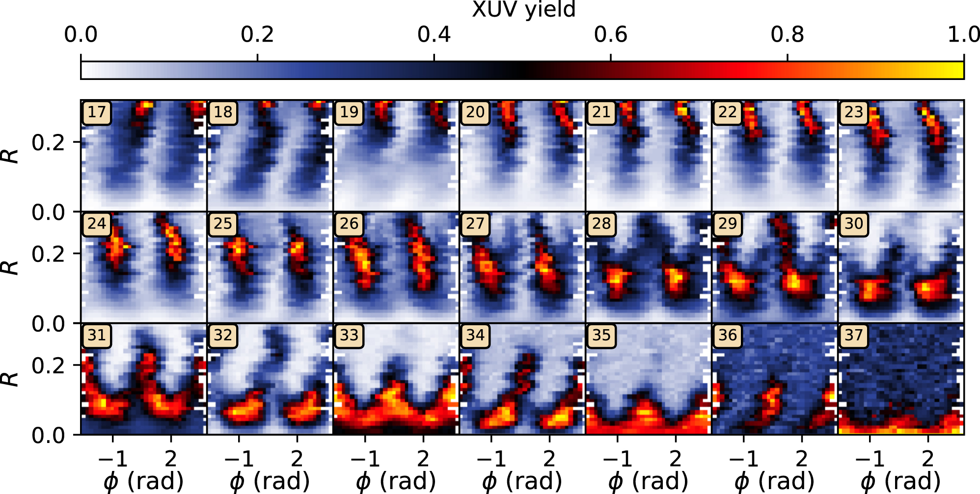
XUV yield for individual harmonic orders, depending on R and ϕ for I _tot = 0.9 × 10¹⁴ W/cm². For each harmonic, with the order indicated by the numbered box, the yield is normalized to its maximum.

2.3 Analysis

To determine R _opt as well as the optimum phase ϕ _opt more accurately, a fit was conducted for every line of experimental data with respect to ϕ according to

A represents the modulation amplitude with ϕ of an harmonic order H, while C represents the constant signal baseline. The measure A + C then represents the maximum yield at ϕ _opt. In Figure 2(a), A + C is shown as a color scale for all harmonic orders within the HHG plateau (H = 18 − 29), as a function of R. The cyan dashed line represents R _opt. Figure 2(b) shows ϕ _opt for all harmonic orders as a function of R on a cyclic color scale. Overlaying the dashed cyan line (R _opt), it becomes evident that the phase values corresponding to this line seem to be constant (white color). These values of ϕ _opt at R _opt are extracted and shown on the right axis as red triangles in Figure 2(c). As soon as a global yield optimum in Figure 1 is reached from H = 23 on, ϕ _opt at R _opt indeed is concentrated around ϕ _opt = −1 rad. This applies only for H > 22, where a global maximum of the yield could be reached. For H < 23 (yellow-filled triangles) the optimum phase at the yield maximum at R = 0.32 is shown instead. The left axis in Figure 2(c) represents the yield enhancement, which is calculated by dividing the yield at R _opt by the yield at R = 0, for odd orders, shown as black stars. For H < 23, a global yield maximum at R _opt could not be reached due to the limitation for R in the experiment; see Figure 1. The stars filled with yellow thus denote the enhancement that was reached at R = 0.32.

Figure 2:

Data analysis results. (a) A + C from Eq. (3) for R and harmonic order (color) within the plateau (H = 18 − 29). The optimum ratio R _opt (cyan dashed line) marks the maximum yield for each harmonic order. (b) ϕ _opt for R and harmonic order (color, cyclic scale). (c) For odd orders, the enhancement of the yield compared to R = 0 is plotted (black stars). The ϕ _opt value at R _opt below the cyan dashed line is extracted and shown on the right axis (red triangles). The stars and triangles filled with yellow H < 23 denote that a global yield maximum was not reached in the experiment.

3.1 Three-step model at ϕ = −1 rad

To understand what is happening at ϕ _opt = −1 rad, the three-step model is evaluated, calculating the electron trajectories for an electric field according to Eq. (2), for varying ionization times T _I and extracting the kinetic energy and the return time T _R of the electrons that recombine with the parent atom, matching the conditions of the experiment with I _tot = 0.9 × 10¹⁴ W/cm². In Figure 3(a)–(d), the corresponding XUV photon energy with I _p = 15.7 eV is shown for different values of R as a function of ϕ and T _R in units of the single-color laser cycle T _ω , for one electric field half-cycle.

Figure 3:

Electron time-energy curves. (a)–(d) E _R + I _p in the unit of harmonic order H for electrons ionized during one electric field half cycle, as a function of ϕ and return time T _R in units of the electric field cycle of the fundamental T _ω , for four examples of R. The cyan line marks the experimentally discovered optimum phase ϕ _opt = −1 rad. (e)–(h) The energy distribution at the position of the cyan lines as line-outs.

E _R + I _p is given in units of the corresponding harmonic order H. For R = 0 (a), which corresponds to a standard single-color field, there is no variation with ϕ and the electrons in the two half-cycles behave identically with respect to their return energy. When R increases, from (a) to (d) in Figure 3, the return energies of the electrons in the first half cycle are suppressed, while they are enhanced for the second one. The location of the largest suppression corresponds to ϕ = −1 rad, which is indicated by the cyan dashed line. The distributions of E _R + I _p corresponding to this line are shown in Figure 3(e)–(h) as line-outs. The essential observation is that this suppression of return energy is what causes an increase of harmonic yield.

The harmonic yield can be estimated by assuming that it is proportional to ( d E R / d T I ) − 1 [17]. This expression diverges for a maximum, such as the cutoff at 3.17U_p for a one-color field with

Here, e is the electron charge and m _e the electron mass. This situation corresponds to the R = 0 line-out in Figure 3 which leads to a rapid decrease of the strength of the harmonic orders in the cutoff region. Such a singularity can also be treated with catastrophe theory [28] in the form of caustics. Caustics in the context of optics describe high concentrations of intensity in a diffraction pattern [30]. In the context of two-color HHG, the enhancement of yield is proportional to the order of the return energy versus return time singularity, which is related to how many orders of derivatives of the curves shown in Figure 3(e)–(h) vanish [27]. Thus, addition of a second harmonic field can suppress the return energies in a certain range of the optical cycle, which flattens the time-energy curve. This makes electrons coalesce to the same energy of the emitted harmonic, which is thus enhanced.

To calculate the harmonic order to which the location of the time-energy curve flattening corresponds, the contributions of ω and 2ω are considered separately. In Figure 4(a), the electric fields are plotted for ϕ = −1 rad at an exemplary ratio of R = 0.2 for ω (red) and 2ω (green). In Figure 4(b), the resulting total electric field according to Eq. (2) for ϕ = −1 rad and different R values is shown. The electric fields hereby correspond to the electron return energy distributions highlighted in (e)–(h) of Figure 3. Figure 4(c) shows the calculated XUV photon energies (E _R + I _p ) in the unit of the corresponding harmonic order, sharing the same color scale as Figure 3, as a function of the ionization T _I and return time T _R at ϕ = −1 rad.

Figure 4:

The three-step model at  ϕ = −1 rad. (a) Electric field for ω (red) and 2ω (green) for ϕ = −1 rad and R = 0.2. (b) Total electric field according to Eq. (2) for different values of R and ϕ = −1 rad. (c) E _R + I _p at the corresponding ionization time T _I and return time T _R at ϕ = −1 rad, sharing the color scale of Figure 3. The approximately constant flattening location with respect to ionization (orange) and return (cyan) is highlighted with solid vertical lines.

The electrons that contribute to the flattening of the time-energy curve are ionized and return approximately at the same times, independently of R. This is indicated by the vertical lines for ionization (orange, T _I = −0.93T _ω ) and recombination (cyan, T _R = −0.295T _ω ). The total field plotted in Figure 4(b) is approximately highest at the time of ionization. At the time of recombination the 2ω contribution is equal to zero, as highlighted in Figure 4(a). Interestingly, the time of return coincides with an isosbestic point of the fields, independent of R. This means that the electric field E(t = T _R , ϕ = −1 rad, R) upon return has the same amplitude. For R = 0.2, which is associated with the highest enhancement of the harmonic order corresponding to the plateau in the time-energy curve (see Figure 3(g)) the first derivative of E _tot also vanishes (pink dashed line).

The absolute value of the velocity v an electron acquires upon recombination is calculated by

with p being the momentum and E _ω , E _2ω given by Eq. (2). For the fundamental ω, the orange and cyan lines in Figure 4 approximately coincide with the times following the classical cutoff energy, with

applying energy conservation and E _R = m _e v ²/2. For R = 0, Eq. (6) corresponds to the well-known cutoff law [17]. For the 2ω component, the vertical lines coincide with the field peak (ionization) and the zero-crossing (recombination), greatly simplifying the evaluation of Eq. (5) and leading to

using the definition of the ponderomotive potential U _p for R = 0.

The XUV photon energy corresponding to electrons at the flat region of E _R versus T _R is expressed as

Solving Eq. (8) for R yields an expression for R _opt depending on the harmonic order corresponding to E _H that is to be enhanced.

3.2 Theory – experiment comparison

In Figure 5, Eq. (8) is compared to the experimental results. The theory is shown as a dashed line and the experimentally found R _opt values are indicated as squares, for I _tot = 0.9 × 10¹⁴ W/cm² (red) and I _tot = 1.35 × 10¹⁴ W/cm² (blue). The shaded areas represent the effect of a 10 % change of I _tot and R in Eq. (8) to highlight the effect of a realistic error margin for optical intensity measurements in an experiment. The red squares hereby correspond to the data shown in Figure 1, for harmonic orders where a global yield maximum could be reached. For I _tot = 1.35 × 10¹⁴ W/cm², the maximum value for R that could be reached experimentally decreased to R = 0.2, only a small amount of second harmonic was available due to the design of the interferometer [29]. As the setup was originally designed for the observation of low-order high harmonics the signal-to-noise ratio after H37 decreases rapidly. Within the shown observation range in Figure 5, the experimental results show excellent agreement with Eq. (8).

Figure 5:

Comparison between Eq. (8) (dashed lines) and experimental results (squares) for I _tot = 0.9 × 10¹⁴ W/cm² (red) and I _tot = 1.35 × 10¹⁴ W/cm² (blue). The shaded areas represent the effect of a 10 % change of I _tot and R in Eq. (8).

The relative yield enhancement compared to R = 0 shown in black in Figure 2(c) seems to be proportional to R _opt (dashed cyan line). The overall best enhancement according to catastrophe theory should occur at the parameters with the largest degree of singularity, which corresponds to the very flat plateau at (R, ϕ) ≈ (0.2, −1 rad) (see Figure 3(g)). In terms of overall yield enhancement (sum of all harmonic orders) the experiment agrees as well with the highest yield at R ≈ 0.2, shown in Figure 2(a). The relatively increasing individual enhancement below H23 can be explained by the very low signal at R = 0 for these harmonics. It is also interesting to notice that our findings in terms of ϕ _opt = −1 rad also correspond to the results shown in Raz et al. for several electric field ratios in a comparable range, measured at a fundamental wavelength of 800 nm and a pulse duration of 30 fs [27], strengthening the validity of our optimization law in Eq. (8).

In our simple model, the change of ionization rate due to the second color is not included. We still consider the model to be valid, since the impact of the second color on the trajectories seems to be more significant than on the ionization rates. Similar observations were also made in an ω/3ω experiment [31].

3.3 Implications for phase-matching

The discussion so far only considered the single-atom response. Thus, the validity of Eq. (8) is independent of other experimental parameters, such as gas target design or pulse duration. The fairest comparison of XUV yield enhancement that can be reached for a harmonic order would be to compare two perfectly phase-matched experimental conditions. This was already realized in a previous work when investigating the influence of relative polarization in a two-color setup, achieving an unexpected higher enhancement for perpendicular polarization than for parallel polarization [12], contradicting conclusions drawn from the three-step model [32].

In this work, the experimental conditions for R = 0 and R ≠ 0 are identical regarding focusing geometries, gas target length, gas pressure, and total intensity to ensure reproducibility. For every R and ϕ variation, the phase matching conditions change as the phase-mismatch due to ionization varies. The sensitivity of the XUV conversion efficiency with these changes depends on the gas target length relative to the Rayleigh length of the laser.

According to Weissenbilder et al., HHG is efficient either for a short gas target with high gas pressure or for a long gas target at lower pressure [20]. In our experiment, the gas target length is estimated to be equal to ≈ 100 µm, which is short compared to the Rayleigh lengths of 2.2 mm (ω) and 1.1 mm (2ω). This places our experiment in the phase-matching regime which strongly depends on the ionization degree in the medium. Assuming that phase-matching is optimized for R = 0, the enhancement, which is obtained for a given (R, ϕ) (see left axis in Figure 2(c)) without changing the generation conditions, might become even larger, if the interaction parameters are adjusted to optimize phase-matching with the two-color field. Such an investigation will require further experiments and theoretical calculations.

References

[1] N. Dudovich, J. L. Tate, Y. Mairesse, D. M. Villeneuve, P. B. Corkum, and M. B. Gaarde, “Subcycle spatial mapping of recollision dynamics,” Phys. Rev. A, vol. 80, no. 1, p. 011806, 2009. https://doi.org/10.1103/physreva.80.011806.Search in Google Scholar
[2] S. D. C. Roscam Abbing, F. Campi, A. Zeltsi, P. Smorenburg, and P. M. Kraus, “Divergence and efficiency optimization in polarization-controlled two-color high-harmonic generation,” Sci. Rep., vol. 11, no. 1, p. 24253, 2021. https://doi.org/10.1038/s41598-021-03657-2.Search in Google Scholar PubMed PubMed Central
[3] E. Mansten, J. M. Dahlström, P. Johnsson, M. Swoboda, A. L’Huillier, and J. Mauritsson, “Spectral shaping of attosecond pulses using two-colour laser fields,” New J. Phys., vol. 10, no. 8, p. 083041, 2008. https://doi.org/10.1088/1367-2630/10/8/083041.Search in Google Scholar
[4] P. Wei, et al.., “Selective enhancement of a single harmonic emission in a driving laser field with subcycle waveform control,” Phys. Rev. Lett., vol. 110, no. 23, p. 233903, 2013. https://doi.org/10.1103/physrevlett.110.233903.Search in Google Scholar PubMed
[5] P. Wei, et al.., “Efficient selection of a single harmonic emission using a multi-color laser field with an aperture-iris diaphragm,” Laser Phys., vol. 24, no. 8, p. 085302, 2014. https://doi.org/10.1088/1054-660x/24/8/085302.Search in Google Scholar
[6] S. Mitra, et al.., “Suppression of individual peaks in two-colour high harmonic generation,” J. Phys. B: At., Mol. Opt. Phys., vol. 53, no. 13, p. 134004, 2020. https://doi.org/10.1088/1361-6455/ab859c.Search in Google Scholar
[7] J. Mauritsson, P. Johnsson, E. Gustafsson, A. L’Huillier, K. J. Schafer, and M. B. Gaarde, “Attosecond pulse trains generated using two color laser fields,” Phys. Rev. Lett., vol. 97, no. 1, p. 013001, 2006. https://doi.org/10.1103/physrevlett.97.013001.Search in Google Scholar PubMed
[8] N. Dudovich, et al.., “Measuring and controlling the birth of attosecond xuv pulses,” Nat. Phys., vol. 2, no. 11, pp. 781–786, 2006. https://doi.org/10.1038/nphys434.Search in Google Scholar
[9] D. Shafir, Y. Mairesse, D. M. Villeneuve, P. B. Corkum, and N. Dudovich, “Atomic wavefunctions probed through strong-field light–matter interaction,” Nat. Phys., vol. 5, no. 6, pp. 412–416, 2009. https://doi.org/10.1038/nphys1251.Search in Google Scholar
[10] M. Fieß, et al.., “Attosecond control of tunneling ionization and electron trajectories,” New J. Phys., vol. 13, no. 3, p. 033031, 2011. https://doi.org/10.1088/1367-2630/13/3/033031.Search in Google Scholar
[11] S. Watanabe, K. Kondo, Y. Nabekawa, A. Sagisaka, and Y. Kobayashi, “Two-color phase control in tunneling ionization and harmonic generation by a strong laser field and its third harmonic,” Phys. Rev. Lett., vol. 73, no. 20, pp. 2692–2695, 1994. https://doi.org/10.1103/physrevlett.73.2692.Search in Google Scholar
[12] I. J. Kim, et al.., “Highly efficient high-harmonic generation in an orthogonally polarized two-color laser field,” Phys. Rev. Lett., vol. 94, no. 24, p. 243901, 2005. https://doi.org/10.1103/physrevlett.94.243901.Search in Google Scholar
[13] T. T. Liu, T. Kanai, T. Sekikawa, and S. Watanabe, “Significant enhancement of high-order harmonics below 10 nm in a two-color laser field,” Phys. Rev. A, vol. 73, no. 6, p. 063823, 2006. https://doi.org/10.1103/physreva.73.063823.Search in Google Scholar
[14] R. A. Ganeev, et al.., “Enhancement of high-order harmonic generation using a two-color pump in plasma plumes,” Phys. Rev. A, vol. 80, no. 3, p. 033845, 2009. https://doi.org/10.1103/physreva.80.033845.Search in Google Scholar
[15] L. Brugnera, et al.., “Enhancement of high harmonics generated by field steering of electrons in a two-color orthogonally polarized laser field,” Opt. Lett., vol. 35, no. 23, pp. 3994–3996, 2010. https://doi.org/10.1364/ol.35.003994.Search in Google Scholar PubMed
[16] C. Porter, et al.., “Soft x-ray: novel metrology for 3D profilometry and device pitch overlay,” in Metrology, Inspection, and Process Control XXXVII, vol. 12496, 2023, pp. 412–420.10.1117/12.2658495Search in Google Scholar
[17] P. B. Corkum, “Plasma perspective on strong field multiphoton ionization,” Phys. Rev. Lett., vol. 71, no. 13, pp. 1994–1997, 1993. https://doi.org/10.1103/physrevlett.71.1994.Search in Google Scholar PubMed
[18] K. J. Schafer, B. Yang, L. F. DiMauro, and K. C. Kulander, “Above threshold ionization beyond the high harmonic cutoff,” Phys. Rev. Lett., vol. 70, no. 11, pp. 1599–1602, 1993. https://doi.org/10.1103/physrevlett.70.1599.Search in Google Scholar PubMed
[19] E. Constant, et al.., “Optimizing high harmonic generation in absorbing gases: model and experiment,” Phys. Rev. Lett., vol. 82, no. 8, pp. 1668–1671, 1999. https://doi.org/10.1103/physrevlett.82.1668.Search in Google Scholar
[20] R. Weissenbilder, et al.., “How to optimize high-order harmonic generation in gases,” Nat. Rev. Phys., vol. 4, no. 11, pp. 713–722, 2022. https://doi.org/10.1038/s42254-022-00522-7.Search in Google Scholar
[21] L. E. Chipperfield, J. S. Robinson, J. W. G. Tisch, and J. P. Marangos, “Ideal waveform to generate the maximum possible electron recollision energy for any given oscillation period,” Phys. Rev. Lett., vol. 102, no. 6, p. 063003, 2009. https://doi.org/10.1103/physrevlett.102.063003.Search in Google Scholar
[22] C. Jin, G. Wang, A.-T. Le, and C. D. Lin, “Route to optimal generation of soft x-ray high harmonics with synthesized two-color laser pulses,” Sci. Rep., vol. 4, no. 1, p. 7067, 2014. https://doi.org/10.1038/srep07067.Search in Google Scholar PubMed PubMed Central
[23] C. Jin, G. Wang, H. Wei, A.-T. Le, and C. D. Lin, “Waveforms for optimal sub-kev high-order harmonics with synthesized two- or three-colour laser fields,” Nat. Commun., vol. 5, no. 1, p. 4003, 2014. https://doi.org/10.1038/ncomms5003.Search in Google Scholar PubMed
[24] K. Schiessl, E. Persson, A. Scrinzi, and J. Burgdörfer, “Enhancement of high-order harmonic generation by a two-color field: influence of propagation effects,” Phys. Rev. A, vol. 74, no. 5, p. 053412, 2006. https://doi.org/10.1103/physreva.74.053412.Search in Google Scholar
[25] Y. Chen, B. Li, X. Li, X. Tang, C. Zhang, and C. Jin, “Effect of laser focus in two-color synthesized waveform on generation of soft x-ray high harmonics,” Chin. Phys. B, vol. 32, no. 1, p. 014203, 2023. https://doi.org/10.1088/1674-1056/ac8cea.Search in Google Scholar
[26] S. Stremoukhov, “Role of gas pressure in quasi-phase matching in high harmonics driven by two-color laser field,” Atoms, vol. 11, no. 7, p. 103, 2023. https://doi.org/10.3390/atoms11070103.Search in Google Scholar
[27] O. Raz, O. Pedatzur, B. D. Bruner, and N. Dudovich, “Spectral caustics in attosecond science,” Nat. Photonics, vol. 6, no. 3, pp. 170–173, 2012. https://doi.org/10.1038/nphoton.2011.353.Search in Google Scholar
[28] M. V. Berry and C. Upstill, “IV catastrophe optics: morphologies of caustics and their diffraction patterns,” in Progress in Optics, vol. 18, E. Wolf, Ed., Amsterdam, Netherlands, Elsevier, 1980, pp. 257–346.10.1016/S0079-6638(08)70215-4Search in Google Scholar
[29] A.-K. Raab, et al.., “Highly versatile, two-color setup for high-order harmonic generation using spatial light modulators,” Rev. Sci. Instrum., vol. 95, no. 7, p. 073002, 2024. https://doi.org/10.1063/5.0212578.Search in Google Scholar PubMed
[30] Y. A. Kravtsov and Y. I. Orlov, “Caustics, catastrophes, and wave fields,” Phys.-Usp., vol. 26, no. 12, pp. 1038–1058, 1983. https://doi.org/10.1070/pu1983v026n12abeh004582.Search in Google Scholar
[31] T. Severt, J. Troß, G. Kolliopoulos, I. Ben-Itzhak, and C. A. Trallero-Herrero, “Enhancing high-order harmonic generation by controlling the diffusion of the electron wave packet,” Optica, vol. 8, no. 8, pp. 1113–1121, 2021. https://doi.org/10.1364/optica.422711.Search in Google Scholar
[32] H. Eichmann, et al.., “Polarization-dependent high-order two-color mixing,” Phys. Rev. A, vol. 51, no. 5, pp. R3414–R3417, 1995. https://doi.org/10.1103/physreva.51.r3414.Search in Google Scholar PubMed
[33] S. Haessler, et al.., “Optimization of quantum trajectories driven by strong-field waveforms,” Phys. Rev. X, vol. 4, no. 2, p. 021028, 2014. https://doi.org/10.1103/physrevx.4.021028.Search in Google Scholar
© 2025 the author(s), published by De Gruyter, Berlin/Boston
This work is licensed under the Creative Commons Attribution 4.0 International License.
Articles in the same Issue
- Frontmatter
- Editorial
- In honor of Federico Capasso, a visionary in nanophotonics, on the occasion of his 75th birthday
- Reviews
- Flat nonlinear optics with intersubband polaritonic metasurfaces
- Polaritonic quantum matter
- Machine-learning-assisted photonic device development: a multiscale approach from theory to characterization
- Perspectives
- Towards field-resolved visible microscopy of 2D materials
- Perspective on tailoring longitudinal structured beam and its applications
- Tunable holographic metasurfaces for augmented and virtual reality
- Polarization-sensitive diffractive optics and metasurfaces: “Past is Prologue”
- Compound meta-optics: there is plenty of room at the top
- Nonlocal metasurfaces: universal modal maps governed by a nonlocal generalized Snell’s law
- Resonant metasurface-enabled quantum light sources for single-photon emission and entangled photon-pair generation
- Active metasurface designs for lensless and detector-limited imaging
- Letter
- Real-time tuning of plasmonic nanogap cavity resonances through solvent environments
- Research Articles
- On the generalized Snell–Descartes laws, shock waves, water wakes, and Cherenkov radiation
- Silicon rich nitride: a platform for controllable structural colors
- Overcoming stress limitations in SiN nonlinear photonics via a bilayer waveguide
- High-harmonic generation from subwavelength silicon films
- Space-time wedges