Tutorial: Hong–Ou–Mandel interference with structured photons

1 Introduction

With the advent of second quantisation, the study of optical elements such as mirrors, wave plates, and beamsplitters, along with their interactions with various quantum states, emerged as a natural domain for exploration. This theoretical framework enabled quantum physicists to rigorously describe and analyze how quantum states evolve under the influence of optical systems, providing deeper insights into quantum optics and discovering novel optical phenomena. An important example is the action of a lossless beamsplitter on photonic quantum states, which was extensively studied by several research groups in the late 1980s. Their theoretical analyses revealed that indistinguishable photons tend to “bunch” together at the output ports of a lossless beamsplitter, a phenomenon now known as the Hong–Ou–Mandel (HOM) effect [1]. The experimental verification of this effect was later carried out by Hong, Ou, and Mandel [2] and independently by Rarity and Tapster [3]. Utilising photons generated through spontaneous parametric down-conversion (SPDC), these experiments not only confirmed the photon bunching effect, but also demonstrated its practical utility in quantum metrology, achieving sub-picosecond temporal precision [4]. Recent advancements have improved these techniques, achieving sub-femtosecond time-resolution capabilities [5].

Single-particle interference raises fundamental questions regarding path determination and the visibility of interference, challenging classical notions of locality in the context of quantum systems, i.e., wave-particle duality. In contrast, multi-particle interference, manifested by the HOM effect, introduces additional layers of foundational complexity, revealing unique many-body quantum features. For instance, the unitary action of a 50:50 beamsplitter on two independent, indistinguishable photons ensures that the photons always emerge from the same output port. This phenomenon arises from destructive quantum interference between two particles that eliminates the possibility of photons exiting through separate output ports, a universal property of lossless beamsplitters irrespective of their physical construction, whether dielectric or metallic. The quantum state of the photons is critical in determining the interference outcomes. For instance, by engineering the quantum state to mimic fermionic behaviour, the photons exhibit anti-bunching, always exiting through different output ports–a unique contrast to their bosonic counterpart [6], [7]. Such manipulations not only highlight the versatility of quantum states but also emphasise the rich interplay between quantum statistics and optical systems. Although a beamsplitter is inherently a linear optical element, it is a fundamental tool for facilitating interactions between multiple photons–a crucial device for quantum information processing. By changing the quantum state of one of the input photons, a beamsplitter (or polarising beamsplitter) can effectively control the output quantum states and the distribution of photons at its ports – varying the reflection and transmission coefficients allows to control the distribution further. This functionality underpins the implementation of a controlled-NOT (CNOT) gate [8], [9], a cornerstone for constructing all-optical quantum circuits.

A single photon carries various degrees of freedom, including polarisation, frequency, and spatial modes. While polarisation spans a two-dimensional vector space, frequency and spatial modes are inherently unbounded, offering infinite-dimensional Hilbert spaces. As a result, the quantum states of two photons may vary across any of these degrees of freedom. When two photons encounter a beamsplitter, the resulting interaction depends critically on the overlap between their quantum wavefunctions [10]. This overlap determines the two-photon interference at the beamsplitter’s output ports. However, the detection systems – such as detectors positioned at the exit ports – and measurement processes introduce further complexities, which require attention. Measurement schemes, driven by the detectors’ sensitivity, can significantly reduce the adequate Hilbert space of the photons to the subspaces detected. For instance, selecting photons within a specific frequency domain by means of bandpass filters reduces the frequency Hilbert space, which can either enhance or diminish the indistinguishability of the photons’ quantum states [1]. Similarly, bucket detectors, which are insensitive to spatial modes, effectively project onto mixed spatial modes, ignoring spatial-mode information altogether. Numerous studies have theoretically and experimentally explored the effects of a beamsplitter on photons characterised by quantum states across different degrees of freedom, such as frequency [11], [12], polarisation [13], orbital angular momentum [14], [15], [16], radial quantum numbers [17], vector modes [18], [19], [20], [21], [22], [23], and waveguide modes [24]. Despite this progress, there remains a gap in the literature: a comprehensive tutorial addressing the interplay between beamsplitters, detection systems, and photons with differing spatial modes. Such a tutorial would be a critical resource for understanding and designing experiments where spatial-mode mismatches and their impact on quantum interference are central considerations. Specifically, an analytical treatment of spatial-mode interference may be computationally advantageous towards the automated search for quantum experiments [25], [26] involving the interference between quantum states with complex spatial amplitudes. With a closed-form, analytical expression of the overlap between such states, we may observe orders of magnitude speedups towards finding new quantum experiments that exploits structured light physics for tasks in precise timing measurements [27], and for the generation of high-dimensional N00N states [28].

This tutorial is organized as follows. In Section 2, we review the theory of multiphoton states, which can be in several different spatial modes – a more detailed review can be found in Ref. [29]. In Section 3, we develop the theory of HOM interference between two frequency-degenerate photons taking into account both their spatial mode content and measurement devices. We specialize the results into different examples that highlight how different measurement configurations allow to recover different information on the bunching photons. In Section 4, we derive an analytical formula for the scalar product of Laguerre–Gauss modes with different mode parameters, which can provide a useful speedup in calculating the outcome of free-space optical quantum networks that we outline in the application Section 5.

2 Multimode quantum optics

The second quantisation of electric and magnetic fields provides a quantum formalism for describing electromagnetic waves at the single quantum level, i.e., photons. In fact, a photon is defined as an excitation of the vacuum state 0 , expressed as:

where a ̂ † and a ̂ denote the creation and annihilation operators for photons, respectively [30], [31]. These operators satisfy the relationships a ̂ † n = n + 1 n + 1 and a ̂ n = n n − 1 , with n representing the quantum state of n photons. In the above notation, the photon’s quantum state is not determined. A single photon possesses several degrees of freedom, such as polarisation, frequency (or time), and spatial modes (transverse position or wave vector). Accordingly, the mode annihilation and creation operators can be labeled with these quantum numbers, i.e., a ̂ σ , ω , q , a ̂ σ , ω , q † . Here, the polarization state σ can take values of { + 1, − 1}, corresponding to the left- or right-handed polarisation states, ω ∈ R stands for the Hilbert frequency space, and q ∈ R 2 refers to the transverse components of the wavevector k = ( q , ω 2 / c 2 − q 2 ) . One can also define creation and annihilation operators in the “transverse position space”, r _⊥, using the Fourier transformation: a ̂ σ , ω , r ⊥ ≔ ∫ d 2 q exp ( − i q ⋅ r ⊥ ) a ̂ σ , ω , q . Of course, a single photon described by a given wavefunction can exist in a coherent or incoherent superposition of these degrees of freedom [30], [32], such as:

where f _σ (r _⊥, ω) is the expansion coefficient function, which can be interpreted as the probability amplitude of detecting a photon with frequency ω and polarization σ in the transverse position r _⊥. For example, the state of a monochromatic, left-handed single photon with a spatial profile given by the Laguerre–Gauss modes [33] can be expressed as:

Here a ̂ + 1 † ( r ⊥ ) is the creation operator that generates a left-handed circularly polarized photon at transverse position r _⊥ in the propagation plane specified by the distance z. The LG _p,ℓ (r _⊥; z) are the LG modes, given by the following expression in cylindrical coordinates (r _⊥; z) = (ρ, ϕ; z),

Here, w ( z ) = w 0 ( 1 + ( z / z 0 ) 2 ) 1 / 2 , R ( z ) = z ( 1 + ( z 0 / z ) 2 ) , z 0 = k w 0 2 / 2 , k and w ₀ are the radius of the beam, the curvature of the beam, the Rayleigh range, the wave vector, and the radius of the beam at the waist, respectively, and L p | ℓ | ( . ) are the generalized Laguerre polynomials. Note that we have neglected the propagation phase factor of exp(i(kz − ωt)). The index ℓ is an integer and is associated with the helical wavefront structure exp(iℓϕ) which implies that these are eigenmodes of the Orbital Angular Momentum (OAM) operator with eigenvalue ℓℏ [34]. The index p is instead a positive integer that counts the number of amplitude zeros in the radial direction [35], [36].

In order to determine Laguerre–Gaussian modes, in addition to radial and azimuthal indices p, ℓ, the beam waist needs to be fixed. Assuming a fixed beam waist w ₀, LG modes form a complete set of orthogonal bases that satisfy the relationships (p, ℓ|p′, ℓ′) = δ _p,p′ δ _ℓ,ℓ′ and ∑ p , ℓ | p , ℓ ) ( p ′ , ℓ ′ | = 1 ̂ – here we use ‘rounded’ kets, |…) to distinguish vectors in the Hilbert space of square integrable functions L 2 ( R 2 ) from elements of the Fock space. It is important to note that two LG modes with different beam waist parameter or with different wavefront curvature, even if possessing different radial indices, are not orthogonal.

In a similar fashion, the quantum states of two or more photons can be described in terms of their respective quantum properties. Depending on the generation, manipulation, configuration, or experimental setup, these photons may share identical or possess different quantum states. For instance, N photons can be prepared in the same spatial, polarisation, or frequency modes (indistinguishable states) or in different modes (distinguishable states). This formalism can be employed to represent separable states, entangled states, and other multi-photon quantum phenomena. To highlight this point, we report here the expression of two cases of N photon states.

N identical photons having the same polarisation state, and spatial modes: Using a ̂ † n = n + 1 n + 1 and Eq. (3) we obtain

N photons having different quantum states:

The difference between these states can be stressed considering the equal-time first-order correlation function, g ( 1 ) ( r ⊥ ) ≔ ψ a ̂ † ( r ⊥ ) a ̂ ( r ⊥ ) ψ , that models intensity measurements. In the case of N photon in the same spatial mode, this yields g ( 1 ) ( r ⊥ ) = LG p , ℓ ( r ⊥ ) 2 , while in the case ψ = ∏ i = 1 N 1 σ i , p i , ℓ i a straightforward calculation shows that g ( 1 ) ( r ⊥ ) = ∑ i LG p i , ℓ i ( r ⊥ ) 2 . Thus, in the first case, an intensity measurement will display the typical shape of an LG mode, while in the second case, one can expect a more ‘blurred’ image arising from the incoherent sum of many different modes.

So far, we have discussed the proper quantum description of multi-photons that can possess various distinct quantum states, such as differing spatial modes, polarisation, or frequency. These photons can possess identical or different quantum states, describing different experiments. Now, we shift our focus to describe the action of optical devices and detectors.

A lossless linear device, e.g. a phase shifter or a beamsplitter, or a waveplate, can be described as a linear transformation mapping the creation operators in a specific mode into a superposition of creation operators in different modes [37]:

where the coefficients u _α,β are the entries of a M × M unitary matrix, with M being the number of modes involved. The unitarity requirement comes from the assumption of the absence of losses, equivalent to the conservation of the number of photons. The indices α, β can refer to different sets of mode labels. The simplest example is the phase shifter that simply multiplies the input mode by a phase factor a ̂ α † → e i θ a ̂ α † . This operation can describe the propagation through a thin slab of material or in free space. However, for long enough propagation ranges, one must take into account that the phase θ can depend on the spatial mode (so it is at least in part conditioned by the index α).

A second example of mode transformation is the beamsplitter, the essential tool for HOM interference. The beamsplitter (BS) is a slab of material tilted with respect to the incident photons at a non-zero angle that can partially reflect and partially transmit light. For a consistent quantum mechanical description of the BS operation, one should consider photons incident on either face of the material. Under the condition that the incidence angles are fixed (with a small uncertainty allowed by the paraxial approximation), the BS acts as a two-input, two-output device. It is also convenient to define with ( a ̂ † , b ̂ † ) the vector of input creation operators of photons entering through port (a, b) (see Figure 1) and with ( c ̂ † , d ̂ † ) the vector of output creation operators of photons exiting through port (c, d) –as for now we do not specify additional mode indices in the creation operators. Conservation of photon number implies that the BS is described by a transformation of the form [38], [39], [40]:

with r 2 + t 2 = 1 . The factors r and t are associated with the reflectivity and the transmissivity of the device (this can be indeed confirmed by calculating the action of the BS on an ideal laser beam, modelled as a coherent state [39]). For instance, a 50/50 dielectric BS will have r = t = 1 / 2 . It is also common to find the choice r = 1 / 2 , t = i / 2 , known as symmetric beam splitter. Note also the minus sign in Eq. (8), which, for bulk dielectric beam splitters, accounts for the well-known π phase shift experienced by electromagnetic waves after reflection. Both choices are physically equivalent, apart from a phase imbalance, which can account for (or be compensated with) differences in path lengths in the input and output arms. In general, several BS representations can be connected via local unitary transformations.

Figure 1:

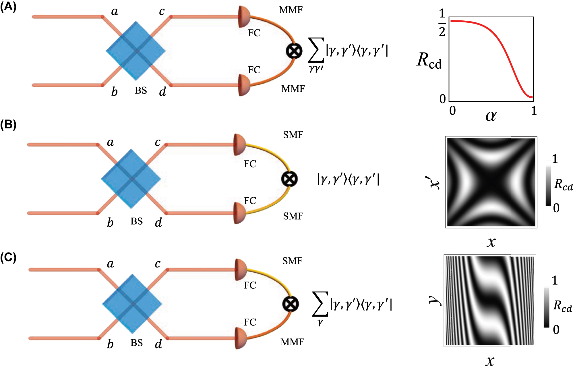
Examples of HOM experimental configurations. Photon pairs enter ports a and b of a beamsplitter, BS, and coincidence counts between the two output paths c and d are collected, typically after coupling to fibres (FC). Each detector can be either a single mode, represented by a single mode fibre (SMF), or a bucket/multimode detector, represented by a multimode fibre (MMF). Panel A shows the case of two bucket detectors and the corresponding coincidence counts as a function of the overlap between input modes. Panel B shows the case of 2 single mode detectors. The inset considers the case in which the detectors are camera pixels and the coincidence count distribution is evaluated for ψ ₁ having a quadratic phase ϕ(x, y) = x ²/w ² with w = 1, according to Eq. (25). Finally, in C, we consider the hybrid case where in one arm there is a bucket detector and in the other a single mode (pixel) detector. The inset shows the coincidence pattern when a phase object O ( x ) = exp ( i ( x 3 + y ) ) is placed in an input port, and correlated photon pairs are used (see Eq. (31)).

For incident fields described by paraxial spatial modes, the coefficients r and t are approximately independent of the incident mode except for the OAM modes. Care must be taken in this case, since the index ℓ changes sign under reflection. A convenient way to address this sign-change without the need to perform cumbersome coordinate transformations, is to choose the subscripts ± ℓ in creation operators in such a way that the output c is associated with −ℓ and d with +ℓ. Thus, for LG modes the BS action can be written as,

The BS is thus the prototypical example of a 2 × 2 unitary operation, i.e. a single qubit gate.

Generic quantum processing protocols can be implemented by combining beamsplitters, phase shifters and measuring devices [37]. The latter completes the toolkit for HOM interference. As we shall see, the outcome of HOM experiments is strongly affected by the choice of detectors. The action of a detector determines how quantum states are measured and influences the results of quantum experiments [30]. A bucket detector is a simple example, and in fact, it is insensitive to the polarization state, frequency, or spatial mode of the incoming photon, meaning that it does not discriminate between these degrees of freedom. The action of a single photon bucket detector effectively projects onto a mixed state, represented as:

When performing a measurement on a quantum system described by the density matrix ρ ̂ ψ , and detecting a single photon without regard to its specific quantum state, the probability of detecting the photon using a bucket detector is given by the following,

where Trace(.) is the trace of the operator, which can be evaluated using any orthonormal basis of convenience. For instance, if ρ is written in terms of LG modes then one can calculate the trace as Trace ( . ) = ∑ p , ℓ p , ℓ ρ ̂ p , ℓ .

If the detector is sensitive to a specific spatial mode, e.g. LG _q,m , and is capable of detecting only one single photon, then the action of the detector is given by

In this case, the probability of detecting a photon from a physical system of ρ ̂ ψ using a detector that is capable of performing a projective measurement of a desired spatial mode of LG _q,m is given by the following,

where in the last step we evaluated the trace in the LG basis and used p , ℓ | q , m = δ p , q δ ℓ , m . With this in mind, we are ready to move on to the description of the HOM effect after different detection conditions.

3 HOM under different detection configurations

After introducing the formalism describing the transformation of electromagnetic field operators by macroscopic lossless media and the effect of projective measurements, the stage is ready to investigate the Hong–Ou–Mandel interference between polarization and frequency-degenerate photons. In this tutorial, we want to stress the effect of the spatial modes involved in the input fields and in the detection stage. The treatment of HOM in the frequency degree of freedom can be found in several references, including Ref. [1].

Input state: Several choices of input states are possible depending on the experimental scenario. Here, we focus on the simplest case of two photons prepared in a product state where each photon enters the beamsplitter from a different port. We later generalize the results to input correlated photon pairs. Let us assume that the photon entering in port a is in the spatial mode ψ ₁(r _⊥) and the photon entering port b is in the spatial mode ψ ₂(r _⊥). This is equivalent to the statement that the input state is of the form ψ 0 = ψ 1 a ⊗ ψ 2 b . The explicit expression of ψ 1,2 depends on the choice of mode decomposition. Let us denote with a ̂ α † a creation operator for photons entering the port a in mode α (to be specified), and with b ̂ β † a creation operator for photons entering the port b in mode β. If α and β are associated with the transverse position then ψ 1 = ∫ d r ⊥ 2 ψ 1 ( r ⊥ ) a ̂ r ⊥ † 0 and ψ 2 = ∫ d r ⊥ 2 ψ 2 ( r ⊥ ) b ̂ r ⊥ † 0 . Alternatively, α and β can be sets of discrete indices associated with orthonormal sets of spatial modes (e.g. ℓ, and p). For instance, a decomposition in LG modes yields ψ 1 = ∑ ℓ , p ( ℓ , p | ψ 1 ) a ̂ ℓ , p † 0 and ψ 2 = ∑ ℓ , p ( ℓ , p | ψ 2 ) b ̂ ℓ , p † 0 . Here we used the notation ( ℓ , p | ψ 1,2 ) ≔ ∫ d 2 r ⊥ LG ℓ , p * ( r ⊥ ) ψ 1,2 ( r ⊥ ) to denote the hermitian product in the space of complex functions with integrable square. In the following calculation, we will not specify whether we choose one or the other mode decomposition:

where the summation symbol has to be intended as an integral if the indices α and β are continuous.

Action of the beamsplitter: We consider for simplicity a 50:50 beamsplitter (BS) acting on the input modes as follows:

where c and d refer to the output ports of the beamsplitter. Thus, the output state is

Measurement: Typical HOM experiments consist of measuring the coincidence counts at the output ports c and d of the BS. This can be formalized as the outcome of a simultaneous projective measurement Π ̂ c d = Π ̂ c ⊗ Π ̂ d . Without losing generality, we can model the projection operators in the form

where, from Π ̂ 2 = Π ̂ (the defining property of projection operators), the real coefficients p _γ must obey p _γ = 0, 1. These different choices allow us to distinguish between bucket, few-mode, and single-mode detectors. The projector operator for coincidence measurements is, thus,

whence the measurement output will be

Note that R _c,d is what one measures when counting in coincidences, normalized to the total number of counts. Often, in HOM experiments, one compares R _c,d with the coincidence counts outside the HOM dip which can be easily measured unbalancing the interferometer, i.e. introducing temporal distingushability between the incoming photons. We now focus on the term 0 c ̂ γ d ̂ γ ′ ψ out . It is evident that, from Eq. (16), only terms with a photon in mode d and a photon in mode c can contribute to R _c,d . The non-zero contribution is

Substituting, we obtain the general result

where is useful to recall that ψ _i,γ = (γ|ψ _i ), with i = 1, 2. In the following section, we specialize this result into three scenarios that can be often encountered in experiments.

4 Explicit formulae for Laguerre–Gauss modes basis

From the previous sections, it is evident how the coincidence rate in HOM experiments requires the evaluation of inner products between spatial modes (ψ ₁|ψ ₂). The completeness and orthogonality of the Laguerre–Gauss modes allows to always expand ψ _1,2 as an infinite series of LG functions. The inner product will thus become a superposition of inner products between different LG modes. Two approaches can be used:

(1) ψ ₁ and ψ ₂ are decomposed in the same LG basis (same choice of waist w ₀ and propagation distance z). In this case, if ψ 1,2 = ∑ ℓ , p A ℓ , p ( 1,2 ) LG ℓ , p , ψ ₁(r _⊥) = LG _l,p (r _⊥; z), then

where we used (ℓ, p|ℓ′, p′) = δ _ℓ,ℓ′ δ _p,p′.

(2) The modes ψ _1,2 may be more conveniently expanded in LG functions with different w ₀ and z for modes 1 and 2. Indeed, the number of relevant coefficients A _ℓ,p can be reduced significantly by looking for an optimal decomposition waist (a nice example for hypergeometric-Gaussian modes is given in Ref. [46]). This situation can be of interest when the modes incident on the beamsplitter have different radii and wavefront curvature, as illustrated in Figure 2. In these scenarios, the product (ℓ, p|ℓ′, p′) in Eq. (32) should be replaced by the complex-valued integral

where

We hereafter introduce w′(z′) and R′(z′) to indicate, respectively, the beam waist and the radius of curvature of the beam at propagation distance z′ and having waist w o ′ and, consequently, Rayleigh range z o ′ . Thus, μ′ is a coefficient that depends on w′(z′). In experiments, if the distances and the characteristics of each optical element before the BS are known, the values of z, z′, w _o and w o ′ can be calculated from the ABCD matrix of the setup (see, e.g. Refs. [33], [47], [48]). From Eq. (4), the explicit formula of the LG modes can be applied directly to the integral. The azimuthal part yields a δ _l,l′2π factor. We, therefore, evaluate the case where l = l′. By performing the substitution x = ρ ², the integral can be put into the following form

where

with Δ ψ G ≔ ( 2 p ′ + | ℓ ′ | + 1 ) arctan z ′ z o ′ − ( 2 p + | ℓ | + 1 ) arctan ( z z o ) is the difference between the accumulated geometric phases.

Figure 2:

Illustration of HOM interference geometry for input photons having different mode parameters.

The integral has an analytical solution expressed in terms of the hypergeometric function ₂ F ₁ [49].

We plot the value of |(l, p|l′p′)|² between different combinations of LG modes in Figure 3a and b (recall that this is associated with the HOM visibility when two bucket detectors are used). The usual orthogonality of modes falls off as we vary the beam waist and relative propagation distance between the beams, and “crosstalk” with other, non-orthogonal LG modes can be observed. We note that experimentally, situations can be achieved where z, z′ ≪ z ₀ with careful alignment. Slight mismatches due to experimental imperfection in the waist parameters can often be met and severely affect the HOM visibility. The analytical formula of Eq. (37) can further be used to explore different, more unconventional experimental scenarios.

Figure 3:

Evaluation of |(l, p|l′p′)|² with l = l′ = 2 and for different combinations of p, p′ ∈ [0, 6]. We demonstrate how the overlap between two beams changes (a) when the ratio of waists and (b) when the relative propagation distance between both beams changes. In both cases, the overlap between identical LG modes falls significantly, and we may observe “crosstalk” with other LG modes. The evaluation of the overlap using the analytical expression demonstrates computational speedup by several orders of magnitude in comparison to a numerical integration using SciPy’s quadrature method.

5 Applications

5.1 Complex quantum networks with spatial modes

Computing the results of a linear network requires the precise evaluation of single- and multi-photon interference effects, predominantly the HOM interference as described here. Conventionally, single-photon interference can also be described in a simple way by taking the local phases of photonic modes into account. This scenario becomes more complex, as spatial modes acquire a propagation-dependent phase that depends on the order of the spatial mode – namely the accumulated Gouy phase [50], [51]. The difference between the accumulated Gouy phase in different paths of the optical network leads to a single-photon interference effect, which has been shown to be useful for sorting spatial modes [52], [53]. They also impact the outcome of two-photon experiments, even in rather simple experimental scenarios, as we show in Figure 4. We explicitly demonstrate this impact for the experimental scenario in Figure 4(a). We start with an incoming state with one photon with equal modes α along the input ports of the first input BS

ψ = 1 a 1 b = a ̂ α † b ̂ α † 0 a 0 b .

After the first BS, we have

ψ = 1 2 ( a ̂ α † + b ̂ α † ) ( a ̂ α † − b ̂ α † ) 0 a 0 b = 1 2 a ′ ̂ α † a ′ ̂ α † − b ′ ̂ α † b ′ ̂ α † 0 a 0 b ,

where a′ and b′ refer to the output ports of the first BS. We then propagate the two modes towards the second BS. We may encode the accumulated Gouy phase difference in terms of a phase-shifting element that encodes an equivalent phase φ _α

a ̂ α † → e i φ α a ̂ α † .

We explicitly included a mode-dependence in the phase φ _α , which is important if this phase is a Gouy phase. For simplicity we will drop the subscript α in the following equations. Therefore, just before the second BS, we have

ψ = 1 2 ( a ′ ̂ † a ′ ̂ † e i 2 φ − b ′ ̂ † b ′ ̂ † ) .

Finally, after application of the second BS,

(38) ψ = 2 ( e i 2 φ − 1 ) 4 ( 2 c 0 d + 0 c 2 d ) + ( e i 2 φ + 1 ) 2 ( 1 c 1 d ) ,

where c and d refer to the output ports of the second beamsplitter. This demonstrates the effect that the accumulated Gouy phase exhibits on the outcome of the interference. Tuning this phase can determine whether we observe a HOM antibunching, as is the case when φ = 0, or if we observe with complete certainty two-photon bunching at the output with φ = − π 2 . We now recall that φ depends on the mode order. Specifically, for LG modes φ = (p + |ℓ| + 1) arctan(z/z ₀), adjusting the interferometer in such a way that z = z ₀ then φ = (p + |ℓ| + 1)π/2, so if p + |ℓ| is odd one observes HOM bunching, while if p + |ℓ| is even one observes antibunching. This could be used to employ HOM as a two-photon parity-mode-sorter, which generalizes the mode sorters demonstrated in Refs. [52], [53]. HOM antibunching has been observed in several experiments where an anti-symmetric distribution in the spatial wavefunction of two photons was used as an input [6], [7], [54].

Figure 4:

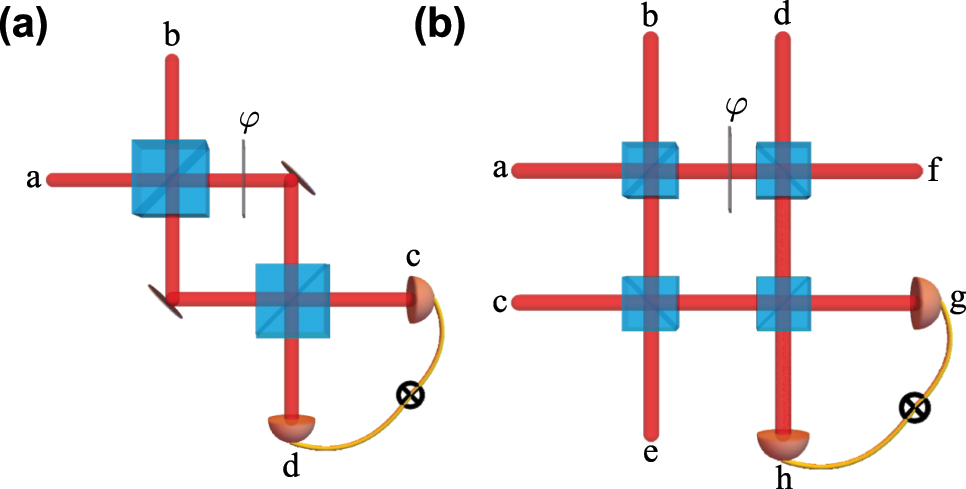
Example experimental scenarios involving (a) two-photon interference with an incoming state ψ i n = 1 a 1 b and (b) multi-photon interference with ψ i n = 1 a 1 b 1 c 1 d . The indices refer to different input ports to the BSs. The accumulated Gouy phase difference between possible paths can be modeled as a phase-shifting element that encodes a phase φ. In both cases, the outgoing state and coincidence rate depend on φ, implicating single-photon interference effects in the outcome of both experiments.

References

[1] Z.-Y. J. Ou, Multi-Photon Quantum Interference, vol. 43, New York, Springer, 2007.Suche in Google Scholar
[2] C.-K. Hong, Z.-Y. Ou, and L. Mandel, “Measurement of subpicosecond time intervals between two photons by interference,” Phys. Rev. Lett., vol. 59, no. 18, p. 2044, 1987, https://doi.org/10.1103/physrevlett.59.2044.Suche in Google Scholar PubMed
[3] J. G. Rarity and P. Tapster, “Fourth-order interference in parametric downconversion,” JOSA B, vol. 6, no. 6, pp. 1221–1226, 1989, https://doi.org/10.1364/josab.6.001221.Suche in Google Scholar
[4] A. Lyons, et al.., “Fluorescence lifetime hong-ou-mandel sensing,” Nat. Commun., vol. 14, no. 1, p. 8005, 2023, https://doi.org/10.1038/s41467-023-43868-x.Suche in Google Scholar PubMed PubMed Central
[5] A. Lyons, et al.., “Attosecond-resolution hong-ou-mandel interferometry,” Sci. Adv., vol. 4, no. 5, p. eaap9416, 2018, https://doi.org/10.1126/sciadv.aap9416.Suche in Google Scholar PubMed PubMed Central
[6] Y. Zhang, F. S. Roux, T. Konrad, M. Agnew, J. Leach, and A. Forbes, “Engineering two-photon high-dimensional states through quantum interference,” Sci. Adv., vol. 2, no. 2, p. e1501165, 2016, https://doi.org/10.1126/sciadv.1501165.Suche in Google Scholar PubMed PubMed Central
[7] X. Gao, Y. Zhang, A. D’Errico, F. Hufnagel, K. Heshami, and E. Karimi, “Manipulating the symmetry of transverse momentum entangled biphoton states,” Opt. Express, vol. 30, no. 12, pp. 21276–21281, 2022, https://doi.org/10.1364/oe.458776.Suche in Google Scholar PubMed
[8] T. Pittman, M. Fitch, B. Jacobs, and J. Franson, “Experimental controlled-not logic gate for single photons in the coincidence basis,” Phys. Rev. A, vol. 68, no. 3, p. 032316, 2003, https://doi.org/10.1103/physreva.68.032316.Suche in Google Scholar
[9] S. Gasparoni, J.-W. Pan, P. Walther, T. Rudolph, and A. Zeilinger, “Realization of a photonic controlled-not gate sufficient for quantum computation,” Phys. Rev. Lett., vol. 93, no. 2, p. 020504, 2004, https://doi.org/10.1103/physrevlett.93.020504.Suche in Google Scholar PubMed
[10] F. Bouchard, et al.., “Two-photon interference: the hong–ou–mandel effect,” Rep. Prog. Phys., vol. 84, no. 1, p. 012402, 2020, https://doi.org/10.1088/1361-6633/abcd7a.Suche in Google Scholar PubMed
[11] Y. Zhang, D. England, A. Nomerotski, and B. Sussman, “High speed imaging of spectral-temporal correlations in hong-ou-mandel interference,” Opt. Express, vol. 29, no. 18, pp. 28217–28227, 2021, https://doi.org/10.1364/oe.432191.Suche in Google Scholar
[12] Y. Chen, S. Ecker, L. Chen, F. Steinlechner, M. Huber, and R. Ursin, “Temporal distinguishability in hong-ou-mandel interference for harnessing high-dimensional frequency entanglement,” npj Quantum Information, vol. 7, no. 1, p. 167, 2021, https://doi.org/10.1038/s41534-021-00504-0.Suche in Google Scholar
[13] Y.-H. Kim, S. P. Kulik, M. V. Chekhova, W. P. Grice, and Y. Shih, “Experimental entanglement concentration and universal bell-state synthesizer,” Phys. Rev. A, vol. 67, no. 1, p. 010301, 2003, https://doi.org/10.1103/physreva.67.010301.Suche in Google Scholar
[14] E. Nagali, et al.., “Optimal quantum cloning of orbital angular momentum photon qubits through hong–ou–mandel coalescence,” Nat. Photonics, vol. 3, no. 12, pp. 720–723, 2009, https://doi.org/10.1038/nphoton.2009.214.Suche in Google Scholar
[15] M. Hiekkamäki and R. Fickler, “High-dimensional two-photon interference effects in spatial modes,” Phys. Rev. Lett., vol. 126, no. 12, p. 123601, 2021, https://doi.org/10.1103/physrevlett.126.123601.Suche in Google Scholar
[16] M. Hiekkamäki, F. Bouchard, and R. Fickler, “Photonic angular superresolution using twisted n00n states,” Phys. Rev. Lett., vol. 127, no. 26, p. 263601, 2021, https://doi.org/10.1103/physrevlett.127.263601.Suche in Google Scholar
[17] E. Karimi, et al.., “Exploring the quantum nature of the radial degree of freedom of a photon via hong-ou-mandel interference,” Phys. Rev. A, vol. 89, no. 1, p. 013829, 2014, https://doi.org/10.1103/physreva.89.013829.Suche in Google Scholar
[18] V. D’Ambrosio, G. Carvacho, I. Agresti, L. Marrucci, and F. Sciarrino, “Tunable two-photon quantum interference of structured light,” Phys. Rev. Lett., vol. 122, no. 1, p. 013601, 2019, https://doi.org/10.1103/physrevlett.122.013601.Suche in Google Scholar PubMed
[19] Z.-F. Liu, et al.., “Hong-ou-mandel interference between two hyperentangled photons enables observation of symmetric and antisymmetric particle exchange phases,” Phys. Rev. Lett., vol. 129, p. 263602, 2022, https://doi.org/10.1103/physrevlett.129.263602.Suche in Google Scholar
[20] Y. Chen, et al.., “Verification of high-dimensional entanglement generated in quantum interference,” Phys. Rev. A, vol. 101, p. 032302, 2020, https://doi.org/10.1103/physreva.101.032302.Suche in Google Scholar
[21] L. Hong, X. Cao, Y. Chen, and L. Chen, “Hong–ou–mandel interference of spin–orbit hybrid entangled photons,” APL Photonics, vol. 8, no. 12, 2023, https://doi.org/10.1063/5.0167016.Suche in Google Scholar
[22] C. Schiano, et al.., “Engineering quantum states from a spatially structured quantum eraser,” Sci. Adv., vol. 10, no. 30, p. eadm9278, 2024, https://doi.org/10.1126/sciadv.adm9278.Suche in Google Scholar PubMed PubMed Central
[23] X. Gao, D. Paneru, F. Di Colandrea, Y. Zhang, and E. Karimi, “Generation of the complete bell basis via hong-ou-mandel interference,” arXiv preprint arXiv:2412.14274, 2024.10.1103/dcxb-ql1rSuche in Google Scholar
[24] A. Mohanty, M. Zhang, A. Dutt, S. Ramelow, P. Nussenzveig, and M. Lipson, “Quantum interference between transverse spatial waveguide modes,” Nat. Commun., vol. 8, no. 1, p. 14010, 2017, https://doi.org/10.1038/ncomms14010.Suche in Google Scholar PubMed PubMed Central
[25] M. Krenn, M. Erhard, and A. Zeilinger, “Computer-inspired quantum experiments,” Nat. Rev. Phys., vol. 2, no. 11, pp. 649–661, 2020, https://doi.org/10.1038/s42254-020-0230-4.Suche in Google Scholar
[26] M. Krenn, J. Landgraf, T. Foesel, and F. Marquardt, “Artificial intelligence and machine learning for quantum technologies,” Phys. Rev. A, vol. 107, no. 1, p. 010101, 2023, https://doi.org/10.1103/physreva.107.010101.Suche in Google Scholar
[27] A. Lyons, et al.., “How fast is a twisted photon?” Optica, vol. 5, no. 6, pp. 682–686, 2018, https://doi.org/10.1364/optica.5.000682.Suche in Google Scholar
[28] J. P. Dowling, “Quantum optical metrology–the lowdown on high-n00n states,” Contemp. Phys., vol. 49, no. 2, pp. 125–143, 2008, https://doi.org/10.1080/00107510802091298.Suche in Google Scholar
[29] C. Fabre and N. Treps, “Modes and states in quantum optics,” Rev. Mod. Phys., vol. 92, p. 035005, 2020, https://doi.org/10.1103/revmodphys.92.035005.Suche in Google Scholar
[30] L. Mandel, Optical Coherence and Quantum Optics, Cambridge, Cambridge University Press, 1995.10.1017/CBO9781139644105Suche in Google Scholar
[31] M. O. Scully and M. S. Zubairy, Quantum Optics, Cambridge, Cambridge University Press, 1997.10.1017/CBO9780511813993Suche in Google Scholar
[32] J. Garrison and R. Chiao, Quantum Optics, Oxford, Oxford Univrsity Press, 2008.10.1093/acprof:oso/9780198508861.001.0001Suche in Google Scholar
[33] A. E. Siegman, Lasers, New York, University Science Books, 1986.Suche in Google Scholar
[34] L. Allen, M. W. Beijersbergen, R. Spreeuw, and J. Woerdman, “Orbital angular momentum of light and the transformation of laguerre-Gaussian laser modes,” Phys. Rev., vol. 45, no. 11, p. 8185, 1992, https://doi.org/10.1103/physreva.45.8185.Suche in Google Scholar PubMed
[35] E. Karimi, et al.., “Radial quantum number of laguerre-gauss modes,” Phys. Rev. A, vol. 89, no. 6, 2014, https://doi.org/10.1103/physreva.89.063813.Suche in Google Scholar
[36] W. N. Plick and M. Krenn, “Physical meaning of the radial index of laguerre-gauss beams,” Phys. Rev. A, vol. 92, no. 6, p. 063841, 2015, https://doi.org/10.1103/physreva.92.063841.Suche in Google Scholar
[37] P. Kok, W. J. Munro, K. Nemoto, T. C. Ralph, J. P. Dowling, and G. J. Milburn, “Linear optical quantum computing with photonic qubits,” Rev. Mod. Phys., vol. 79, no. 1, pp. 135–174, 2007, https://doi.org/10.1103/revmodphys.79.135.Suche in Google Scholar
[38] S. Prasad, M. O. Scully, and W. Martienssen, “A quantum description of the beam splitter,” Opt. Commun., vol. 62, no. 3, pp. 139–145, 1987, https://doi.org/10.1016/0030-4018(87)90015-0.Suche in Google Scholar
[39] Z. Ou, C. Hong, and L. Mandel, “Relation between input and output states for a beam splitter,” Opt. Commun., vol. 63, no. 2, pp. 118–122, 1987, https://doi.org/10.1016/0030-4018(87)90271-9.Suche in Google Scholar
[40] H. Fearn and R. Loudon, “Quantum theory of the lossless beam splitter,” Opt. Commun., vol. 64, no. 6, pp. 485–490, 1987, https://doi.org/10.1016/0030-4018(87)90275-6.Suche in Google Scholar
[41] F. Devaux, A. Mosset, P.-A. Moreau, and E. Lantz, “Imaging spatiotemporal hong-ou-mandel interference of biphoton states of extremely high schmidt number,” Phys. Rev. X, vol. 10, no. 3, p. 031031, 2020, https://doi.org/10.1103/physrevx.10.031031.Suche in Google Scholar
[42] X. Gao, Y. Zhang, A. D’Errico, K. Heshami, and E. Karimi, “High-speed imaging of spatiotemporal correlations in hong-ou-mandel interference,” Opt. Express, vol. 30, no. 11, pp. 19456–19464, 2022, https://doi.org/10.1364/oe.456433.Suche in Google Scholar PubMed
[43] R. Chrapkiewicz, M. Jachura, K. Banaszek, and W. Wasilewski, “Hologram of a single photon,” Nat. Photonics, vol. 10, no. 9, pp. 576–579, 2016, https://doi.org/10.1038/nphoton.2016.129.Suche in Google Scholar
[44] G. Thekkadath, D. England, F. Bouchard, Y. Zhang, M. Kim, and B. Sussman, “Intensity interferometry for holography with quantum and classical light,” Sci. Adv., vol. 9, no. 27, p. eadh1439, 2023, https://doi.org/10.1126/sciadv.adh1439.Suche in Google Scholar PubMed PubMed Central
[45] S. P. Walborn, C. Monken, S. Pádua, and P. S. Ribeiro, “Spatial correlations in parametric down-conversion,” Phys. Rep., vol. 495, nos. 4-5, pp. 87–139, 2010, https://doi.org/10.1016/j.physrep.2010.06.003.Suche in Google Scholar
[46] G. Vallone, “Role of beam waist in laguerre–gauss expansion of vortex beams,” Opt Lett., vol. 42, no. 6, pp. 1097–1100, 2017, https://doi.org/10.1364/ol.42.001097.Suche in Google Scholar
[47] A. Yariv, P. Yeh, and A. Yariv, Photonics: Optical Electronics in Modern Communications, vol. 6, New York, Oxford University Press, 2007.Suche in Google Scholar
[48] B. E. Saleh and M. C. Teich, Fundamentals of Photonics, New Jersey, John Wiley & Sons, 2019.Suche in Google Scholar
[49] I. S. Gradshteyn and I. M. Ryzhik, Table of Integrals, Series, and Products, New York, Academic Press, 2014.Suche in Google Scholar
[50] M. F. Erden and H. M. Ozaktas, “Accumulated gouy phase shift in Gaussian beam propagation through first-order optical systems,” JOSA A, vol. 14, no. 9, pp. 2190–2194, 1997, https://doi.org/10.1364/josaa.14.002190.Suche in Google Scholar
[51] K. Arai, “On the accumulated round-trip gouy phase shift for a general optical cavity,” LIGO Tech. Note, vol. 1300189, no. LIGO-T1300189, pp. 1–11, 2013.Suche in Google Scholar
[52] Y. Zhou, et al.., “Sorting photons by radial quantum number,” Phys. Rev. Lett., vol. 119, no. 26, p. 263602, 2017, https://doi.org/10.1103/physrevlett.119.263602.Suche in Google Scholar PubMed
[53] X. Gu, M. Krenn, M. Erhard, and A. Zeilinger, “Gouy phase radial mode sorter for light: concepts and experiments,” Phys. Rev. Lett., vol. 120, no. 10, p. 103601, 2018, https://doi.org/10.1103/physrevlett.120.103601.Suche in Google Scholar PubMed
[54] S. Walborn, A. De Oliveira, S. Pádua, and C. Monken, “Multimode hong-ou-mandel interference,” Phys. Rev. Lett., vol. 90, no. 14, p. 143601, 2003, https://doi.org/10.1103/physrevlett.90.143601.Suche in Google Scholar
[55] M. Krenn, M. Malik, R. Fickler, R. Lapkiewicz, and A. Zeilinger, “Automated search for new quantum experiments,” Phys. Rev. Lett., vol. 116, no. 9, p. 090405, 2016, https://doi.org/10.1103/physrevlett.116.090405.Suche in Google Scholar
[56] P. Knott, “A search algorithm for quantum state engineering and metrology,” New J. Phys., vol. 18, no. 7, p. 073033, 2016, https://doi.org/10.1088/1367-2630/18/7/073033.Suche in Google Scholar
[57] C. Ruiz-Gonzalez, et al.., “Digital discovery of 100 diverse quantum experiments with pytheus,” Quantum, vol. 7, p. 1204, 2023, https://doi.org/10.22331/q-2023-12-12-1204.Suche in Google Scholar
[58] M. Krenn, Y. Drori, and R. X. Adhikari, “Digital discovery of interferometric gravitational wave detectors,” arXiv preprint arXiv:2312.04258, 2023.Suche in Google Scholar
[59] M. W. Mitchell, J. S. Lundeen, and A. M. Steinberg, “Super-resolving phase measurements with a multiphoton entangled state,” Nature, vol. 429, no. 6988, pp. 161–164, 2004, https://doi.org/10.1038/nature02493.Suche in Google Scholar PubMed
[60] P. Walther, J.-W. Pan, M. Aspelmeyer, R. Ursin, S. Gasparoni, and A. Zeilinger, “De broglie wavelength of a non-local four-photon state,” Nature, vol. 429, no. 6988, pp. 158–161, 2004, https://doi.org/10.1038/nature02552.Suche in Google Scholar PubMed
[61] T. Nagata, R. Okamoto, J. L. O’brien, K. Sasaki, and S. Takeuchi, “Beating the standard quantum limit with four-entangled photons,” Science, vol. 316, no. 5825, pp. 726–729, 2007, https://doi.org/10.1126/science.1138007.Suche in Google Scholar PubMed
[62] I. Afek, O. Ambar, and Y. Silberberg, “High-noon states by mixing quantum and classical light,” Science, vol. 328, no. 5980, pp. 879–881, 2010, https://doi.org/10.1126/science.1188172.Suche in Google Scholar PubMed
[63] S. Slussarenko, et al.., “Unconditional violation of the shot-noise limit in photonic quantum metrology,” Nat. Photonics, vol. 11, no. 11, pp. 700–703, 2017, https://doi.org/10.1038/s41566-017-0011-5.Suche in Google Scholar
[64] A. Kuzmich and L. Mandel, “Sub-shot-noise interferometric measurements with two-photon states,” Quantum Semiclassical Opt. J. Eur. Opt. Soc. Part B, vol. 10, no. 3, p. 493, 1998, https://doi.org/10.1088/1355-5111/10/3/008.Suche in Google Scholar
[65] M. Hiekkamäki, R. F. Barros, M. Ornigotti, and R. Fickler, “Observation of the quantum gouy phase,” Nat. Photonics, vol. 16, no. 12, pp. 828–833, 2022, https://doi.org/10.1038/s41566-022-01077-w.Suche in Google Scholar
[66] V. D’ambrosio, et al.., “Photonic polarization gears for ultra-sensitive angular measurements,” Nat. Commun., vol. 4, no. 1, p. 2432, 2013, https://doi.org/10.1038/ncomms3432.Suche in Google Scholar PubMed PubMed Central
© 2025 the author(s), published by De Gruyter, Berlin/Boston
This work is licensed under the Creative Commons Attribution 4.0 International License.
Artikel in diesem Heft
- Frontmatter
- Editorial
- In honor of Federico Capasso, a visionary in nanophotonics, on the occasion of his 75th birthday
- Reviews
- Flat nonlinear optics with intersubband polaritonic metasurfaces
- Polaritonic quantum matter
- Machine-learning-assisted photonic device development: a multiscale approach from theory to characterization
- Perspectives
- Towards field-resolved visible microscopy of 2D materials
- Perspective on tailoring longitudinal structured beam and its applications
- Tunable holographic metasurfaces for augmented and virtual reality
- Polarization-sensitive diffractive optics and metasurfaces: “Past is Prologue”
- Compound meta-optics: there is plenty of room at the top
- Nonlocal metasurfaces: universal modal maps governed by a nonlocal generalized Snell’s law
- Resonant metasurface-enabled quantum light sources for single-photon emission and entangled photon-pair generation
- Active metasurface designs for lensless and detector-limited imaging
- Letter
- Real-time tuning of plasmonic nanogap cavity resonances through solvent environments
- Research Articles
- On the generalized Snell–Descartes laws, shock waves, water wakes, and Cherenkov radiation
- Silicon rich nitride: a platform for controllable structural colors
- Overcoming stress limitations in SiN nonlinear photonics via a bilayer waveguide
- High-harmonic generation from subwavelength silicon films
- Space-time wedges
- XUV yield optimization of two-color high-order harmonic generation in gases
- Skyrmion bag robustness in plasmonic bilayer and trilayer moiré superlattices
- Quantum-enhanced detection of viral cDNA via luminescence resonance energy transfer using upconversion and gold nanoparticles
- Deep neural networks for inverse design of multimode integrated gratings with simultaneous amplitude and phase control
- Topological chiral-gain in a Berry dipole material
- Diagnostic oriented discrimination of different Shiga toxins via PCA-assisted SERS-based plasmonic metasurface
- Quantum emitter interacting with a dispersive dielectric object: a model based on the modified Langevin noise formalism
- 3D-printed mirror-less helicity preserving metasurface “mirror” for THz applications
- Supershift properties for nonanalytic signals
- Enhancing radiative heat transfer with meta-atomic displacement
- Quasi-bound states in the continuum in finite waveguide grating couplers
- Long lived surface plasmons on the interface of a metal and a photonic time-crystal
- Tailoring propagation-invariant topology of optical skyrmions with dielectric metasurfaces
- Experimental generation of optimally chiral azimuthally-radially polarized beams
- Tailoring optical response of MXene thin films
- Nonlinear analog processing with anisotropic nonlinear films
- Optical levitation of Janus particles within focused cylindrical vector beams
- Large tuning of the optical properties of nanoscale NdNiO3 via electron doping
- Combining quantum cascade lasers and plasmonic metasurfaces to monitor de novo lipogenesis with vibrational contrast microscopy
- Monoclinic nonlinear metasurfaces for resonant engineering of polarization states
- Non-linear bistability in pulsed optical traps