Carbon Taxes and CO2 Emissions: A Replication of Andersson (American Economic Journal: Economic Policy, 2019)
-
Yanxia Yu


Abstract
Do carbon taxes reduce CO2 emissions in the countries that adopt it? Andersson (2019. Carbon taxes and CO2 emissions: Sweden as a case study. American Economic Journal: Economic Policy, 11(4), 1–30) provides a clear, affirmative answer. His article has been widely cited as evidence that carbon taxes “work.” To check whether the estimates from Andersson (2019) are reliable, I replicate his article using its publicly available data and codes. I modify his synthetic control method (SCM) by using a more restricted set of control units (excluding one potentially treated unit). I also use a more efficient methodology, the Prais-Winsten estimator, to estimate price effects on gasoline consumption. In addition, I compute prediction intervals (PIs) and add these to the SCM estimates, using the newly developed scpi R package. My best estimate is that carbon taxes reduced per-capita CO2 emissions in Sweden’s transport sector by 7.7%, confirming Andersson’s main finding. I then extend Andersson’s approach to the Norwegian transport sector, estimating a smaller reduction of 2.4%. However, this effect falls within the PIs of the estimates assuming no carbon taxes. When I extend the analysis to the national level in Sweden, I estimate wide PIs and obtain inconclusive results.
1 Introduction
The carbon tax is a market-based policy instrument that aims to reduce energy-related CO2 emissions stemming from fossil fuel consumption. It taxes fossil fuels based on their carbon content, thereby establishing a price for CO2 pollution. This approach aligns with the “polluter pays” principle (Metcalf, 2021), offering the potential for cost-efficient environmental benefits. In the early 1990s, Denmark, Finland, the Netherlands, Norway, and Sweden became the first countries in the world to adopt carbon taxes (Tirkaso & Gren, 2020). Consequently, these countries have attracted the attention of researchers investigating the effectiveness of carbon taxes as a means of mitigating CO2 emissions.
A common approach is to use regression to estimate the effect of carbon taxes on energy consumption (Davis & Kilian, 2011; Enevoldsen et al., 2007; Li et al., 2014; Tirkaso & Gren, 2020). Given this estimate, the reduction in energy consumption can then be translated to a corresponding reduction in CO2 emissions.
A concern with this approach is endogeneity. To address this concern, other studies have treated the introduction of carbon taxes as a quasi-natural experiment and adopted a difference-in-differences (DID) approach (Lin & Li, 2011; Metcalf, 2019; Pretis, 2022). This approach relies on dividing countries/jurisdictions into treatment and control units. CO2 emissions are observed over a period before the carbon tax is adopted (pre-treatment) and after the carbon tax is adopted (post-treatment). The control countries/jurisdictions are chosen to represent the counterfactual, providing an estimate of the potential outcome (what CO2 emissions would have been) if the treatment country had not adopted a carbon tax.
Crucial to the DID approach is the assumption of parallel trends (PT). In a recent article, Andersson (2019) focussed on the Swedish transport sector and noted that pre-treatment growth rates of CO2 emissions were different for control and treatment units in violation of the assumption of PT. Accordingly, he adopted a two-pronged approach.
His main analysis employed a synthetic control method (SCM) to estimate the effect of carbon taxes and the Value-added Tax (VAT) on CO2 emissions. He then used regression analysis of the price elasticity of gasoline consumption to disentangle the effect of VAT from that of carbon taxes. He concluded that the combined effect of extending the VAT to gasoline and diesel and introducing a carbon tax reduced CO2 emissions in the Swedish transport sector by almost 11%, with approximately 6% coming solely from the carbon tax.
The Andersson (2019) study is noteworthy for several reasons. First, it finds a significant impact of carbon taxes on CO2 emissions where previous studies had not (Green, 2021). Second, it studies Sweden, which is often raised as a model for using carbon taxes to mitigate CO2 emissions. And finally, it has been very influential. It has been cited over 450 times in Google Scholar (as measured on April 2, 2024). It received the “Best Paper Award” from the American Economic Journal: Economic Policy, chosen among all articles published in the journal from 2019 to 2021. The award specifically highlighted its implications for public policy by noting that “The effects were larger than previous research had shown, suggesting that policymakers were underestimating the upside of implementing carbon pricing policies” (American Economic Association, 2022).
Given its influence and implications for public policy, it is important to confirm that Andersson’s results are reliable. As Duvendack et al. (2015) note, “there has been a recognition in the economics profession that many empirical results in economics are not reproducible or not generalizable to alternative empirical specifications, econometric procedures, extensions of the data, or other study modifications.” Accordingly, this study follows Mueller-Langer et al. (2019)’s call for the need for “post-publication quality checks in addition to the pre-publication peer review process.”
Drawing upon Clemens’ (2017) framework, my analysis employs a comprehensive approach encompassing four types of replications and robustness tests: verification, reproduction, reanalysis, and extension. For verification, I run Andersson’s (2019) data and code to confirm that they produce the results reported in his article. I also go back to his primary data sources and re-assemble his data set from first principles. For reproduction, I modified the data underlying his analysis by dropping Denmark from his comparison group, which also instituted a carbon tax at about the same time.
For reanalysis, I apply two new methods for data analysis. The first is the Prais-Winsten estimator to estimate gasoline consumption, which accounts for serial correlation. The second one employs the newly developed R package scpi to obtain prediction intervals (PIs) for the SCM estimates. This allows me to assess whether random error could account for the differences between observed emissions under the carbon tax and those estimated from synthesized scenarios assuming no carbon tax.
Finally, I extend Andersson’s analysis in two directions. First, I apply his same procedure to the Norwegian transport sector, which also implemented a carbon tax at this time. Second, I expanded the analysis to include not just the transport industry, but the whole country of Sweden to see if the reduction in CO2 emissions was sufficient to be noticeable at the country level.
My analysis leads me to conclude that Andersson’s findings for Sweden’s transport sector are reproducible and robust. My best estimate is slightly larger than Andersson’s. I estimate that the carbon tax reduced CO2 emissions in the Swedish transport sector on average by 7.7%. My extension analysis, however, finds only a small effect of carbon taxes in Norway’s transport sector (2.4%). Further, the estimated effect lies inside a PI associated with emissions under a no carbon tax regime. When I further extend the analysis to consider country-level emissions for all of Sweden, I obtain inconclusive estimates with wide PIs. Thus, my analysis is unable to find evidence of the effectiveness of carbon taxes beyond the Swedish transport sector studied by Andersson. This suggests that Sweden’s carbon tax experience may not be representative of the effects of carbon taxes elsewhere.
This article proceeds as follows. Section 2 gives background and context for the introduction of carbon taxes in Sweden. Section 3 discusses the datasets and empirical methods used in this analysis. Section 4 replicates Andersson’s results for the Swedish transport sector. Section 5 extends Andersson’s approach to the Norwegian transport sector. Section 6 further extends Andersson’s approach to a country-level analysis of Sweden covering all sectors. Section 7 produces the PIs for the SCM estimates. Section 8 concludes by summarizing my key results and what they contribute to our understanding of carbon taxes and CO2 emissions.
2 Sweden’s Carbon Tax
In March 1990, Sweden extended the VAT to gasoline and petrol, with the real (inflation-adjusted) tax rate subsequently held constant. In 1991, it implemented a carbon tax as part of the Environmental Tax Reform, becoming one of the first countries in the world to do so. Simultaneously with the introduction of carbon taxes, energy taxes on fossil fuels were reduced by 25–50%. The implementation of multiple tax policies at roughly the same time makes it difficult to isolate the separate impact of carbon taxes.
Energy taxes and carbon taxes have been central to Sweden’s environmental policy for the past 30 years. Having been modified several times since its implementation, the carbon tax in Sweden today is characterized by a high tax rate that is predominantly levied on fossil fuels used as motor fuel and for heating purposes (Samuel et al., 2020). When first introduced, the carbon tax rate was 30 USD per ton of CO2 (Andersson, 2019). This rate was gradually increased to around 44 USD in 2000. It experienced a sharp increase in the early 2000s, rising to around 140 USD in 2017, the highest level of carbon taxation in the world (IEA, 2019).
Exemptions have been an important part of the Swedish tax system. Before 2005, fuels used for electricity production were exempted from the carbon tax. The tax rate for the manufacturing industry was set to 25% of other sectors in 1993 and exempted from the general energy tax due to concerns about international competitiveness and carbon leakage (Andersen et al., 2001).[1] Taking exemptions into account, the Swedish carbon tax covers approximately 40% of Sweden’s greenhouse gases.
3 Data and Methods
3.1 Data
The data and code used by Andersson (2019) are posted at: https://www.aeaweb.org/articles?id=10.1257/pol.20170144. The materials were well documented and clearly explained. Data were provided for 15 OECD countries (excluding Norway), with Sweden being the treated unit and the other 14 carefully chosen OECD countries serving as controls. Andersson set the time of treatment as 1990, the year when the VAT was introduced.
As part of my verification analysis, I attempted to retrieve all data from the original data sources in Andersson (2019). My goal was to build up a dataset for 16 OECD countries (including Norway) for the period 1960–2005. This would enable me to confirm that the data used by Andersson could be recreated from the original sources, so that a researcher working from the same data sources would get the same results. I also needed to be certain that the same variables were available for Norway as part of my extension analysis. In doing so, I discovered that data on the level of CO2 emissions from transport are no longer available in the World Bank WDI database (2020). As a result, I sought alternative data sources.
Andersson subsequently made available to me the original data he downloaded from the World Bank WDI Database (2015). These were virtually identical to the data publicly packaged with Andersson (2019) (Table 1), which also includes CO2 emissions for Norway’s transport sector. My extension analysis relies on these latter data.
Summary statistics for replication of Andersson (2019)
| Variable | Data source | Average over | N | Mean | Std. Dev. | Min | Max |
|---|---|---|---|---|---|---|---|
| CO2 emissions from transport (metric tons per capita) | The World Bank WDI Database (2015)a | 1960–2005 | 690 | 2.070 | 1.335 | 0.200 | 6.057 |
| The World Bank WDI Database (2015)b | 1960–2005 | 690 | 2.071 | 1.336 | 0.200 | 6.057 | |
| The World Bank WDI Database (2020), IEAc | 1971–2005 | 525 | 2.387 | 1.367 | 0.513 | 6.210 | |
| Real GDP per capita (2005 USD) | Penn World Table 8.0a | 1980–1989 | 150 | 18,801 | 6,520 | 4,996 | 31,421 |
| Penn World Table 8.0c | 1980–1989 | 150 | 18,801 | 6,520 | 4,996 | 31,421 | |
| Motor vehicles (per 1000 people) | Dargay, Gately, and Sommer (2007)a | 1980–1989 | 150 | 402.6 | 157.5 | 86.21 | 775.5 |
| Dargay, Gately and Sommer (2007)c | 1980–1989 | 150 | 402.6 | 157.5 | 86.21 | 775.5 | |
| Gasoline consumption per capita | WDI (2015)a | 1980–1989 | 150 | 427.6 | 316.8 | 76.30 | 1,250 |
| NationMasterc | 1980–1989 | 150 | 427.6 | 316.8 | 76.30 | 1,250 | |
| Urban population (%) | WDI (2015)a | 1980–1989 | 150 | 75.76 | 12.36 | 42.78 | 96.29 |
| WDI (2020)c | 1980–1989 | 150 | 76.43 | 11.92 | 42.78 | 96.29 |
In order to base my analysis as much as possible on publicly available data, I also indirectly calculated CO2 emissions from transport (million metric tons) as the product of “CO2 emissions from fuel combustion” (from IEA) and “CO2 emissions from transport (% of total fuel combustion)” (from the 2020 World Bank WDI Database). The compiled CO2 emissions data from transport starts from 1971, while the WDI data from Andersson dates to 1960. The values of the constructed CO2 emissions variable are very similar, with a difference of only 0.6% on average over the period 1971–2005. My initial analysis uses these publicly sourced, CO2 emissions data.
Later, I use Andersson’s emissions data from 1960 to 2005. The longer pre-treatment period enables me to better assess whether emissions from the synthetic control follow that of the treated unit. It also allows me to be more consistent with Andersson (2019) in my extension to Norway. For all the other variables, I use the publicly available data that I directly retrieved from the original sources.
Aside from past emissions data, Andersson’s SCM analysis relies on the following set of predictor variables: real GDP per capita, number of motor vehicles, gasoline consumption, and urban population. The data for the predictors cover the years 1980–1989. Table 1 provides summary statistics of Andersson’s dataset and my compiled dataset for the 15 OECD countries (excluding Norway). As shown in the table, my compiled data and Andersson’s data are identical for the first three predictors, and only slightly different for Urban Population.
3.2 Synthetic Control Method
The SCM was originally proposed in Abadie and Gardeazabal (2003) and Abadie et al. (2010) to estimate the effect of large-scale or aggregate interventions. It uses a data-driven approach to construct a control unit (synthetic control), which is a weighted average of the untreated units in the donor pool. The intuition is that the combination of unaffected units provides a more appropriate comparison than any single unaffected unit alone. The following is the basic framework of SCM.
Suppose there are
A set of weights
where
Notice that equation (2) includes a vector of coefficients
When this distance, namely the mean squared prediction error (MSPE) is small, the outcomes for the treated and synthetic control will follow a similar trend. Then, the synthetic control estimate of the treatment effect
The validity of the SCM relies on the “convex hull assumption,” which states that the values of predictors for the treated unit
When the above assumptions are fulfilled, SCM provides an alternative estimation method to DID when the assumption of PT for treatment and control units is suspect. As Andersson (2019) notes,
“The parallel trends assumption is difficult to verify, which is a drawback for the DiD method. It is sometimes possible pretreatment by analyzing the trends of the outcome variable, but obviously impossible after treatment. When the treated unit and the control group do not follow a common trend, the DiD estimator will be biased. Therefore, finding a method that relaxes the parallel trends assumption is preferable for comparative case studies” (page 10).
By reweighting the controls to match the pre-treatment trends in the treated unit, SCM increases the likelihood that the parallel trends assumption holds (Bonander et al., 2021). The other merits of SCM include providing data-driven and formal criteria for selecting control units, showing us the contribution of each control unit in constructing the synthetic control, and the relative importance of the predictors in predicting the pre-treatment outcomes. Although classic SCM does not produce standard errors and confidence intervals, it is common for researchers to conduct in-time, in-space, and leave-one-out placebo tests (Abadie et al., 2010, 2011).
3.3 Regression Analysis
While SCM constitutes the main focus of Andersson’s analysis, he also employs a regression analysis of gasoline consumption. The regression analysis has two uses. First, it provides a robustness test of the SCM analysis. In the absence of endogeneity, the two methods should produce similar estimated effects. The regression analysis also allows one to isolate the separate effects of the VAT and the carbon tax. This is important given that it is the latter which is of primary interest.
Previous research recognizes the possibility that tax-induced price changes may generate distinct demand responses compared with equivalent, market-determined price movements (Rivers & Schaufele, 2015). This phenomenon is called “tax salience.” In the Swedish case, gasoline consumption could respond differently to a rise in gasoline prices induced by the introduction of VAT and a rise due to the carbon tax. Andersson’s analysis allowed for this possibility.
Specifically, he estimated a log-linear gasoline demand model. The retail price of gasoline was decomposed into the carbon tax-exclusive price
where
To address the possible endogeneity of gasoline prices, Andersson used crude oil prices and the energy tax rate as instruments for the carbon tax-exclusive gasoline price and performed two-stage least squares estimation. Based on the regression results, Andersson conducted a simulation, in which he approximated the amount of (counterfactual) CO2 emissions in three cases: Sweden without carbon taxes and VAT, Sweden with VAT but no carbon taxes, and Sweden with carbon taxes and VAT. In the simulation, I multiply gasoline consumptions (kg) by the emission factor of gasoline to get simulated CO2 emissions.[2] The gasoline consumptions under Case 1 and Case 2 are predicted from the gasoline consumption-price regression. Then, the difference in the simulated emissions between Case 2 and Case 3 identifies the effect of carbon taxes on CO2 emissions.
4 Replication and Robustness Tests of Andersson’s Results for the Swedish Transport Sector
4.1 Verification with Andersson’s Data and Code
As noted above, Andersson (2019) provided his data and code as supplementary materials to his published journal article. This allowed me to confirm that his results were “push-button” replicable. Because I obtained identical results to him, I do not report a side-by-side comparison of Andersson’s original results and my replication.
4.2 SCM with Alternative Synthetic Swedens
Figure 1a is a replication of Figure 4 in Andersson (2019). It sets 1990, the year when the VAT was extended to gasoline and diesel, as the treatment year. Figure 1a demonstrates that synthetic Sweden successfully reproduced the trajectory of CO2 emissions for Sweden before the treatment. As shown in the graph, per-capita CO2 emissions from transport in Sweden experienced an immediate drop after 1990 compared to what would have been expected without a carbon tax. The emission gap between Sweden and synthetic Sweden increased gradually in the early 1990s and then remained constant. The resulting average reduction in CO2 emissions from transport in Sweden is −0.29 metric tons per capita, which accounts for 10.9% of the emissions in the absence of VAT and carbon taxes on average.
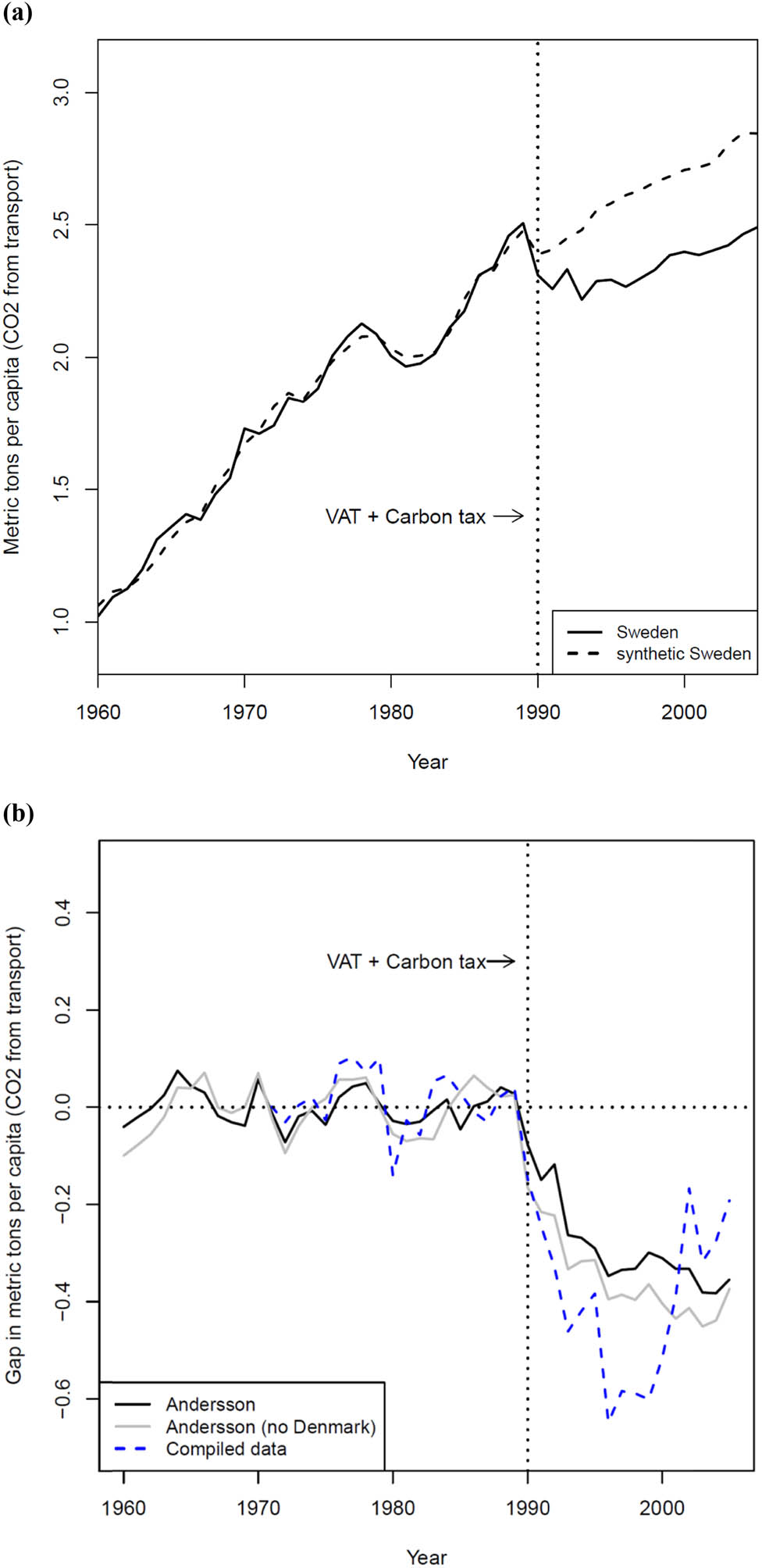
SCM analysis (Swedish Transport). (a) Replication of Andersson’s Figure 4. (b) Three Synthetic Swedens.
My replication of Figure 1a adds two additional synthetic control groups. In addition to Andersson’s control group, I created a second control group that drops Denmark from the donor pool. Denmark introduced a carbon tax on energy products in 1992, though it exempted the transport industry. Andersson, noting that the carbon tax rate was relatively low, decided to keep it in the donor pool. However, Denmark has the largest weight in the construction of its synthetic Sweden. Therefore, I check how conclusions may change if Denmark is excluded from the control group. My third synthetic Sweden uses the data I compiled and reported in Table 1.
Figure 1b recasts Figure 1a in terms of differences in CO2 emissions from transport between actual Sweden and the three synthetic counterparts. As shown in the figure, when Denmark is excluded from the donor pool, the gap becomes wider. This is consistent with the bias one would expect from including a carbon tax adopter in the controls, which would mute the estimated effect of the carbon tax.
Table 2 reports the values for the predictors corresponding to the three synthetic control analyses above.[3] The first four columns reproduce the results in Table 1 of Andersson (2019). They show that compared to the population-weighted average of the 14 OECD countries, Andersson’s synthetic Sweden more closely resembles Sweden with respect to the means of the predictors and per-capita CO2 emissions during the pre-treatment years.
Predictor Means and Weights: SCM analysis (Swedish Transport Sector)
| Replication of Andersson | Excluding Denmark | Compiled data (inc. Denmark) | ||||||||
|---|---|---|---|---|---|---|---|---|---|---|
| Variables | (1) Sweden | (2) Synth. Sweden | (3) OECD sample | (4) Predictor weights | (5) Sweden | (6) Synth. Sweden | (7) Predictor weights | (8) Sweden | (9) Synth. Sweden | (10) Predictor weights |
| GDP per capita | 20121.5 | 20121.2 | 21277.8 | 0.219 | 20121.5 | 20984.8 | 0.005 | 20121.5 | 20123.9 | 0.062 |
| Motor vehicles (per 1,000 people) | 405.6 | 406.2 | 517.5 | 0.078 | 405.6 | 423.9 | 0.029 | 405.6 | 406.3 | 0.27 |
| Gasoline consumption per capita | 456.2 | 406.8 | 678.9 | 0.01 | 456.2 | 442.0 | 0.268 | 456.2 | 417.6 | 0.018 |
| Urban population | 83.1 | 83.1 | 74.1 | 0.213 | 83.1 | 82.8 | 0.092 | 83.1 | 83.1 | 0.177 |
| CO2 From transport per capita 1989 | 2.5 | 2.5 | 3.5 | 0.183 | 2.5 | 2.5 | 0.081 | 2.6 | 2.6 | 0.044 |
| CO2 from transport per capita 1980 | 2.0 | 2.0 | 3.2 | 0.284 | 2.0 | 2.1 | 0.425 | 2.0 | 2.1 | 0.03 |
| CO2 From transport per capita 1970 | 1.7 | 1.7 | 2.8 | 0.013 | 1.7 | 1.7 | 0.1 | 1.8 | 1.8 | 0.40 |
| MSPE | 0.0012 | 0.0026 | 0.0037 | |||||||
| ATT | −0.286 | −0.351 | −0.391 | |||||||
Note: The third column shows the population-weighted average of the 14 OECD countries (Andersson, 2019).
Columns (5)–(7) of Table 2 show that when we exclude Denmark from the donor pool, the predictor values of the synthetic counterpart are still close to that of Sweden, while the MSPE increases slightly from 0.0012 to 0.0026. It indicates that we are able to reduce potential bias at a small cost. For this reason, going forward, my analysis excludes Denmark from the donor pool.
Returning to Figure 1b, we see that when I use the data that I compiled rather than Andersson’s data, the emissions gap is larger in the early 1990s but decreases in the late 1990s. The corresponding average treatment effect is −0.39 metric tons, larger than what Andersson reports (−0.29 metric tons).
Columns (8)–(10) of Table 2 present data on the predictors using my compiled data. While the overall values are similar to Andersson (2019), the corresponding synthetic Sweden has a poorer fit during the pre-treatment years (MSPE of 0.0037 versus 0.0012 and 0.0026). Given that the goodness of fit is worse for the compiled data, the subsequent analysis will use Andersson’s data, excluding Denmark.
4.3 Regression Analysis of Gasoline Consumption Using an Alternative Estimator
When SCM is used in Andersson (2019), by its nature, two effects could not be distinguished: the introduction of a carbon tax in Sweden and the adoption of the VAT in gasoline and diesel, both of which coincided. What further complicates this case is other tax changes that affected gasoline during the post-treatment period. As the tax rate of the carbon tax rose in 2000, it was accompanied by a simultaneous decrease in the tax rate of the energy tax.
In order to separate out the price effects of the carbon tax from the VAT and general price increases, Andersson estimates a demand equation for gasoline consumption that includes both components. To estimate this equation, he uses time series data on Brent Crude oil prices and gasoline consumption from 1970 to 2011. To address endogeneity, he uses two instruments: the energy tax rate and the price of crude oil. However, the IV estimates are similar to the OLS estimates and a Hausman test finds no statistical difference, so he concludes that endogeneity is not a problem.
To account for autocorrelation, Andersson (2019) used the Newey-West procedure to obtain “serial correlation-robust” standard errors for the OLS estimates. Alternatively, I adopt the Prais-Winsten estimation procedure, which is a form of generalized least squares (GLS). Its key assumption is that the errors follow a first-order autoregressive process. In practice, the Prais-Winsten method first estimates the correlation between the errors at
Table 3 presents my verification of the regression analysis in Andersson’s article. The results in columns (1), (2), and (3) are exactly the same as in the study by Andersson (2019). Additionally, Column (4) shows the Prais-Winsten regression results. Across Table 3, the two price components (“Carbon tax-exclusive gasoline price” and “Carbon tax”) have negative and statistically significant coefficients.
Gasoline consumption regressions (Swedish Transport Sector)
| (1) | (2) | (3) | (4) | |
|---|---|---|---|---|
| OLS | IV (EnTax) | IV (OilPrice) | Prais-Winsten | |
| Gas price with VAT | −0.060*** | −0.062*** | −0.064*** | −0.046*** |
| (0.012) | (0.020) | (0.014) | (0.009) | |
| Carbon tax | −0.186*** | −0.186*** | −0.186*** | −0.107** |
| (0.043) | (0.038) | (0.038) | (0.048) | |
| Dummy carbon tax | 0.100 | 0.098 | 0.095 | 0.040 |
| (0.066) | (0.070) | (0.059) | (0.052) | |
| Trend | 0.034*** | 0.034*** | 0.034*** | 0.003 |
| (0.003) | (0.003) | (0.003) | (0.010) | |
| GDP per capita | −0.004*** | −0.004*** | −0.004*** | 0.001 |
| (0.001) | (0.001) | (0.001) | (0.001) | |
| Urban population | 0.030 | 0.031 | 0.033 | −0.007 |
| (0.067) | (0.064) | (0.058) | (0.050) | |
| Unemployment rate | −0.024*** | −0.024*** | −0.024*** | 0.006 |
| (0.006) | (0.005) | (0.005) | (0.008) | |
| Constant | 4.407 | 4.313 | 4.198 | 6.505 |
| (5.446) | (5.152) | (4.693) | (4.018) | |
| Observations | 42 | 42 | 42 | 42 |
| R 2 | 0.76 | 0.76 | 0.76 | — |
Note: Standard errors in parentheses *p < 0.10, **p < 0.05, and ***p < 0.01.
According to the Prais-Winsten estimates in Column (4), if the carbon tax and the non-tax price components each increase by one Swedish Krona, gasoline consumption would decrease by 10.7 and 4.6%, respectively. These effects are smaller in size compared to Andersson’s estimates, which are 18.6 and 6.0%, respectively. I note that Prais-Winsten assumes that the error terms are AR(1). However, there is mixed evidence that the error terms follow a higher order autoregressive process. In that case, Prais-Winsten should still improve efficiency over OLS/Newey-West, which makes no adjustment for serial correlation in its coefficient estimates.
Based on the estimates in Column (1), Table 3, Andersson (2019) approximated CO2 emissions from three scenarios.
As shown in Figure 2a, my calculation produces results quite similar to Andersson (2019). It indicates that the effect of the VAT remained relatively constant after its extension to gasoline in 1990. On the other hand, the effect of the carbon tax experienced a significant increase after 2000 as the real tax rate increased from 0.92 SEK/liter in 2000 to 2.11 SEK/liter in 2005. As Andersson (2019) noted, the sharp increase reflects the separate effect of carbon tax while keeping the (real) rate of energy tax constant. Figure 2b replicates Figure 14 in the study by Andersson (2019) by comparing the effects of carbon tax and VAT from the SCM and the simulation based on OLS regression. Note that the estimated VAT + Carbon tax emission effects from the SCM and regression analyses are quite similar, especially in the first half of the post-treatment period when the real tax rate of the energy tax remained constant.
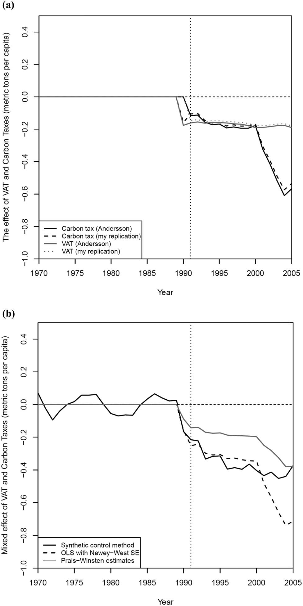
Disentangling the effects of VAT and Carbon Tax (Swedish Transport). (a) Regression Analysis. (b) SCM and Regression Analysis.
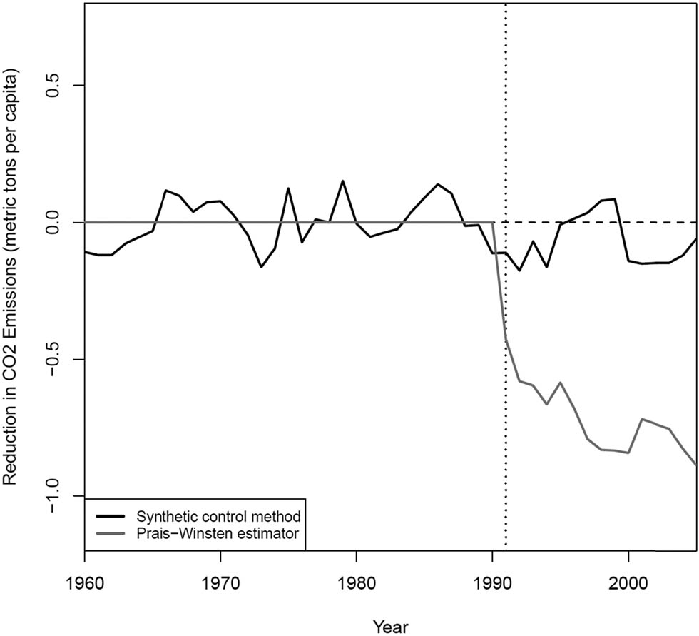
Figure 2b also adds my estimates of emission reduction based on the Prais-Winsten price estimates. The associated reduction is only half the size of the estimated emission reduction from the SCM and the OLS estimates over most of the treatment period. This is a direct consequence of the smaller estimated price and tax effects in Column (4) of Table 3. However, it also shows a sharp increase in impact after 2,000 due to increasing carbon taxes.
Andersson (2019) used the price estimates to assign the proportions of total emission reduction estimated from the SCM (−0.29 metric tons) to VAT and to carbon taxes. He concluded that carbon taxes alone reduced per-capita CO2 emissions from transport in Sweden by 6.3% (0.17 metric tons) on average in the post-treatment period. I repeat this calculation based on my synthetic control analysis (without Denmark) and the Prais-Winsten estimates, and conclude that the Swedish carbon taxes alone reduced CO2 emissions from transport by 7.7% (0.21 metric tons).
Why is a larger estimated emission effect of the carbon tax obtained, compared to Andersson (2019), despite estimating a smaller coefficient of the carbon tax from using the Prais-Winsten method (cf. Table 3)? The reason is that according to the simulated counterfactual emissions, the Swedish carbon taxes account for 59% of the mixed emission reduction from VAT + carbon tax on average during 1991–2005. This share is roughly the same as that from Andersson’s approach (60% on average). As my SCM estimate (without Denmark) is larger, the resulting carbon tax-induced emission reduction is larger. Following Andersson, I apply this larger share to the SCM estimate of the total effect, and that produces a larger carbon tax estimate. While Andersson (2019) fortuitously found that his SCM and regression estimates were similar, he placed greater confidence in the SCM estimates and used the results for the regression analysis solely to determine the split between VAT and carbon taxes. This issue will reappear later when I extend Andersson’s analysis to Norway’s transport sector.
In conclusion, while I modify Andersson’s analysis in several substantive ways, my final estimate of the effect of carbon taxes on CO2 emissions ends up being very close to the 6.3% reduction Andersson estimated.
5 Extension #1 of Andersson (2019) – Norwegian Transport Sector
In this section, I report the results of the first of two extension analyses. I apply the same methodology and predictors to investigate the relationship between carbon taxes and CO2 emissions in Norway’s transport sector, as Norway also adopted a carbon tax.
5.1 Norway’s Carbon Tax
Norway levied CO2 taxes on petroleum, mineral fuel, and natural gas in 1991. In 1991, the tax rate was 39.6 USD per ton of CO2 for natural gas offshore on the continental shelf, 35 USD for oil offshore on the continental shelf and 15–17 USD for heating oil. Petrol was also subjected to a heavy tax of 259 NOK per ton of CO2 (namely, 40 USD/ton) (Andersen et al., 2001). After the implementation, CO2 tax on petrol had increased steadily to a rate of 405 NOK per ton of CO2 (46 USD/ton) in 2,000 and 336 NOK per ton of CO2 (52 USD/ton) in 2005. It is worth noting that the initial rate of Norwegian CO2 tax on petrol was even higher than that of Sweden’s, while it grew more slowly than Sweden’s. This leads to an interesting comparison to Sweden’s carbon tax.
Similarly to Sweden, there are extensive exemptions and differentiation of carbon tax rates in Norway (Bruvoll & Larsen, 2004; Lin & Li, 2011). Since Norway is one of the world’s major oil and natural gas producers and exporters, 29% of total CO2 emissions from oil and gas extraction in 2001 (Statens, 2003). Carbon taxes on oil and gas extraction are set at a comparatively high level, 49 USD for natural gas and 43 USD for oil in 1999 (Bruvoll & Larsen, 2004). Other high-polluting industries, such as the metal-producing industry, are partly or totally exempted for fear of losing competitiveness. There are also exemptions for fishing, air, and ocean transport. As a result, only 60% of the total CO2 emissions in Norway are subjected to CO2 tax. On average, tax revenue from CO2 emissions accounts for 16.9% of total environmental tax revenues.
5.2 SCM Analysis
The predictor variables. The first step in the SCM analysis is choosing a set of predicting variables to construct a synthetic Norway. I apply the same predictors used for constructing synthetic Sweden: real GDP per capita, Motor vehicles (per 1,000 people), Gasoline consumption per capita, Urban population (%), per-capita CO2 emissions from transport in 1970, 1980, and 1989. Table 4 shows the values of the key predictors in the pre-treatment period. The majority of the weights (75%) are given to the past values of CO2 emissions.
Predictor means and weights: SCM analysis (Norwegian Transport Sector)
| Variables | Norway | Synth. Norway | OECD sample | Weight |
|---|---|---|---|---|
| GDP per capita | 22470.4 | 21247.7 | 18531 | 0.043 |
| Motor vehicles (per 1,000 people) | 409.3 | 421.3 | 406.9 | 0.193 |
| Gasoline consumption per capita | 372.6 | 408.7 | 436.0 | 0.009 |
| Urban population | 71.2 | 91.0 | 75.3 | 0 |
| CO2 from transport per capita 1989 | 2.5 | 2.5 | 2.4 | 0.271 |
| CO2 from transport per capita 1980 | 2.1 | 2.1 | 2.2 | 0.195 |
| CO2 from transport per capita 1970 | 1.7 | 1.6 | 1.7 | 0.289 |
In contrast, the number of motor vehicles and urban population receive weights of 0.9 and 0%, respectively. It seems as if these two predictors do not play much of a role in predicting per-capita CO2 emissions from transport in Norway. Nevertheless, I decide to keep them on the predictor list to maintain comparability with Andersson (2019).
Overall, Table 4 suggests that synthetic Norway is a better comparison group than the simple average of the untreated, OECD countries. According to the weights given to the 13 OECD countries, synthetic Norway is best reproduced by a combination of Belgium (0.771), Switzerland (0.113), and the United States (0.116).
Checking the parallel trends assumption in the pre-treatment period. While we are unable to test the assumption of PT in the post-treatment period, it is possible to check for it in the pre-treatment period. Figure 3a compares per-capita CO2 emissions from Norway’s transport sector with the average per-capita CO2 emissions from transport for the 13 OECD countries. It is clear from the figure that the PT assumption does not hold during the pre-treatment period because Norway’s per-capita CO2 emissions clearly grew faster than the OECD average. This provides support for using SCM over DID or a two-way fixed effects model.

SCM analysis (Norwegian Transport). (a) Norway and the OECD average. (b) Norway and Synthetic Norway.
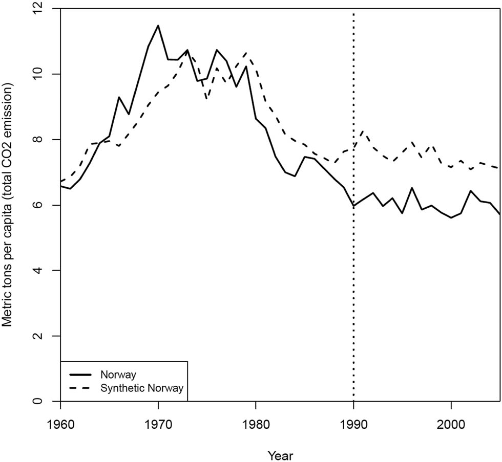
Results from the SCM analysis. Figure 3b shows the results from SCM applied to Norway’s transport sector. CO2 emissions in Norway and synthetic Norway follow a common trend prior to 1990 and diverge after 1990. In 1990, 1 year before the implementation of Norwegian CO2 tax, per-capita CO2 emissions from transport in Norway dropped below that of synthetic Norway. This is consistent with there being an anticipation effect prior to the actual implementation of the carbon tax.
Contrary to Sweden, the SCM analysis finds that emissions in the Norwegian transport sector exceeded that of the synthetic control counterfactual during the years 1996–1999. This constitutes evidence against the effectiveness of carbon taxes to reduce CO2 emissions. Nevertheless, I still estimate an accumulated effect of 0.96 metric tons of emission reduction per capita over the full, 1991–2005, post-treatment period. The corresponding annual per-capita emission reduction is −0.064 metric tons and is on average 2.4% lower than the scenario without the carbon tax. My conclusion is that the Norwegian carbon tax had an overall small, negative effect on per-capita CO2 emissions from transport in Norway.
Placebo robustness tests. To check the credibility of the SCM results for Norway, I conduct placebo tests. For the in-time placebo tests, the treatment is assigned to the years 1970 and 1980. Figure 4 shows that although the fits are not perfect, possibly due to the large variations in the outcome, there is no sign of placebo effects after 1970 and 1980.
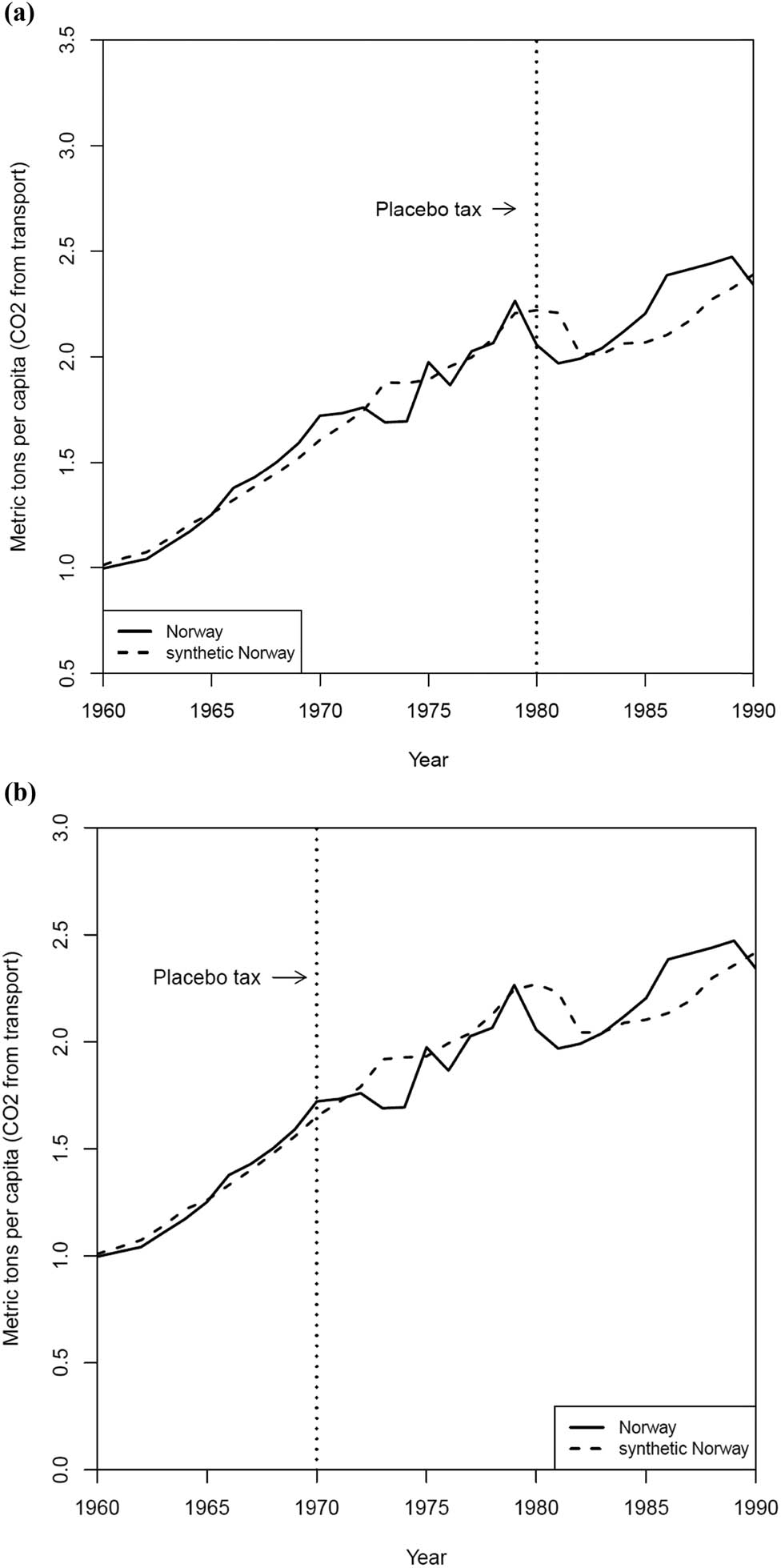
In-time placebo tests (Norwegian Transport). (a) Year of Intervention is 1970. (b) Year of Intervention is 1980.
The in-space placebo test iteratively assigns the treatment to untreated countries in the donor pool and compares the sizes of the resulting “treatment” effects. Figure 5a shows that when we focus on seven placebo units (including Norway) with MSPEs less than 0.01, the effect in Norway (−0.064 metric tons per capita) is the second largest, smaller than Switzerland with a placebo effect of −0.24 metric tons per capita. The “treatment” effects for the other placebo units are either close to zero or positive.
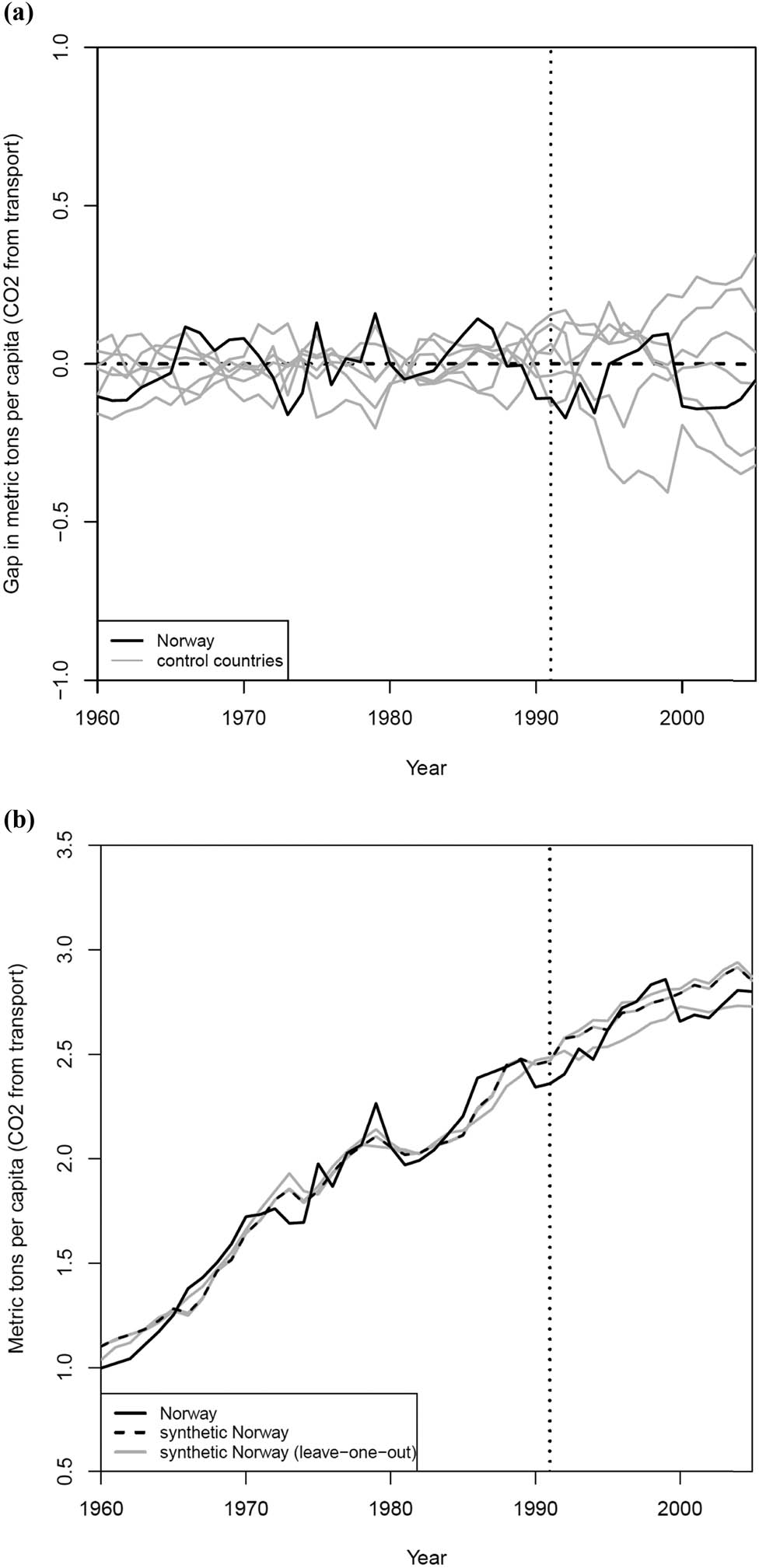
In-space and leave-one-out placebo tests (Norwegian Transport). (a) In-Space Placebo Test. (b) Leave-One-Out Placebo Test.
Figure 5b shows the results of the leave-one-out placebo test, in which the untreated units with positive weights are dropped from the donor pool one at a time to reconstruct the synthetic controls. This practice gives us a range of the estimated effects of carbon tax on per-capita CO2 emissions from transport in Norway, which is −0.093 to −0.037 metric tons per capita. These placebo tests prove the robustness of my baseline results.
Possible confounders. Andersson noted that economic growth could be a confounder that affected his estimates of the impact of the Swedish carbon tax. While SCM is not well-suited to handle confounders, I nevertheless follow Andersson’s approach to investigate whether Norwegian economic performance might bias the carbon tax effect estimated by SCM analysis.
For constructing a synthetic Norway’s real GDP per capita, the same weights used for the synthetic Norway’s CO2 emissions per capita are applied. As shown in Figure 6, the relative trends in per-capita CO2 emissions from transport and per-capita real GDP in Norway were closely co-moving from the late-1980s to the early-1990s (grey-shaded area in the figure). This suggests that the observed downturn in CO2 emissions in 1990 might not have been an “anticipatory effect” associated with the introduction of the carbon tax, but rather was a reflection of a relative downturn in Norwegian economic activity. If so, by spuriously attributing this to the carbon tax, SCM overstates its impact.

Co-movements between GDP and CO2 emissions (Norwegian Transport).
On the other hand, starting in the mid-1990s and continuing through to the end of the post-treatment period, Norway’s actual GDP per capita did substantially better than synthetic Norway. To the extent that the increased, relative economic activity contributed to greater CO2 emissions, SCM analysis understates the impact of the carbon tax. While it is possible that the economy is a confounder, the mixed effects described above do not provide clear evidence that SCM either under- or over-estimates the emission effects of the carbon tax for the Norwegian transport sector.
In conclusion, while I find a small, overall negative effect on emissions due to the carbon tax in the Norwegian transport industry, the higher emissions of the Norwegian transport sector compared to its synthetic control counterfactual from 1996 to 1999 is noteworthy.
5.3 Regression Analysis
As noted above, Andersson (2019) used regression analysis to disentangle the effect of the carbon tax from other taxes. Fortuitously, the overall, estimated effect of VAT + carbon tax from his regression analysis was approximately equal to that of the SCM analysis.
There is no need to do the same for Norway because the introduction of carbon taxes in 1991 was not accompanied by major changes in other taxes that might affect the SCM analysis. Nevertheless, in order to maintain comparability with Andersson (2019), I use regression analysis to calculate an alternative estimate of the emissions effect of Norway’s carbon tax.
Andersson (2019) used annual time series data for Sweden from 1970 to 2011. In contrast, the data available to me only span the period from January 1995 to December 2017, though most of the variables are available monthly. Statistics Norway provides monthly data on gasoline prices, motor gasoline consumption, and quarterly data, which are used for the control variables in this regression analysis, resulting in a dataset of 276 observations. The data on the carbon tax rate are from the IEA (2009).
Table 5 shows the estimation results. The OLS estimates with Newey-West standard errors are shown in Column (1), indicating that a one Norwegian Krone (NOK) increase in the real carbon tax-exclusive gasoline price and carbon tax would result in decreases in gasoline consumption of 2.3 and 27.3%, respectively. Column (2) shows the Prais-Winsten estimates. The coefficients for the real carbon tax-exclusive price and carbon tax are −0.019 and −0.289, both statistically significant at the 1% level. This means that one NOK increase in the carbon tax is estimated to reduce gasoline consumption by 28.9%. In contrast, if the gasoline price rises by one NOK yet this change is not caused by the carbon tax, gasoline consumption would only decrease by 1.9%.
Gasoline consumption regressions (Norwegian Transport Sector)
| (1) | (2) | (3) | |
|---|---|---|---|
| OLS | Prais-Winsten | IV(OilPrice) | |
| Carbon tax-exclusive price | −0.023*** | −0.019** | −0.024* |
| (0.009) | (0.008) | (0.013) | |
| Carbon tax | −0.273*** | −0.289*** | −0.272*** |
| (0.063) | (0.047) | (0.069) | |
| Unemployment | 0.005 | 0.005 | 0.005 |
| (0.009) | (0.006) | (0.011) | |
| Urban population | 0.021 | 0.019 | 0.021 |
| (0.039) | (0.026) | (0.047) | |
| Real GDP (ln) | 2.04*** | 1.998*** | 2.039*** |
| (0.263) | (0.194) | (0.317) | |
| Time trend | −0.007*** | −0.007*** | −0.007*** |
| (0.001) | (0.001) | (0.001) | |
| Constant | −20.54*** | −19.93*** | −20.53*** |
| (3.727) | (2.133) | (3.625) | |
| Month dummy | Yes | Yes | Yes |
| Observations | 276 | 276 | 276 |
| R 2 | 0.98 | — | 0.98 |
Note: Column (1) shows the OLS estimates with Newey-West standard errors. Standard errors in parentheses *p < 0.10, **p < 0.05, and ***p < 0.01.
Column (3) presents results from instrumental variable (IV) estimation, using crude oil prices as an instrument for the carbon tax-exclusive price. As with Sweden, the results are quite similar to the OLS estimates in Column (1). A test for weak instruments shows that the crude oil price is not a weak instrument.
Assuming a roughly one-to-one exchange rate between the Norwegian Krone and the Swedish Krona, these estimated price effects suggest that gasoline consumption is more responsive to carbon taxes in Norway. Also, the persistent finding that carbon taxes have a larger impact than other price components of gasoline is consistent with the estimates from Sweden and “tax salience” theory.
Using the Prais-Winsten estimates in Column (2), I simulated CO2 emissions from Norway’s transport sector in two scenarios: with carbon tax and without carbon tax. The effect of a Norwegian carbon tax in reducing per-capita CO2 emissions is obtained by taking the difference between these two scenarios, which is −0.55 metric tons per capita on average during 1991–2005. This effect size accounts for 27% of per capita CO2 emissions from transport that would occur without a carbon tax. In light of the SCM estimates this seems implausibly large (Figure 7 for a comparison of the two methods).
Comparing SCM and regression (Norwegian Transport).
As I obtained two contrasting estimates from two different methods, a natural question is: To which should one attach greater weight? There are reasons to prefer the SCM estimate. First, despite efforts to address endogeneity bias through IV estimation, there remain concerns about misspecification and endogeneity with regression estimates of a gasoline demand equation. This was why Andersson (2019) preferred his SCM estimates to the regression estimates. But there is a second reason to prefer SCM.
The regression analysis is based solely on gasoline consumption. It does not include diesel consumption. CO2 emissions from road transportation in Norway increased 19% from 1990 to 2001. This rise is primarily attributed to an increase of 73% in emissions from diesel, whereas emissions from gasoline vehicles decreased by 7% during this period (Statens, 2003).[4] This substitution from gasoline to diesel is not captured in the regression analysis, which focuses solely on the carbon tax effect on gasoline consumption. In contrast, SCM has the advantage of capturing the impact on emissions for the whole transport sector, not just the portion due to gasoline consumption and its attendant CO2 emissions.
In conclusion, I estimate that the carbon tax had different effects on the transport sector in Sweden and Norway: a relatively large effect for Sweden, and a relatively small effect for Norway (as shown in Table 7). The reasons for this difference are not clear. The goal of this analysis was to extend Andersson’s methods to see if I could obtain similar results for Norway.
6 Extension #2 of Andersson (2019) – Total Sweden Impact
The previous analysis focused on emissions from the transport sector. This section investigates the impact of carbon taxes on per capita, total CO2 emissions for all of Sweden – not just the transport sector. The reason for extending the analysis to all of Sweden is this: If carbon taxes are able to reduce CO2 emissions to a meaningful extent, we should be able to see its effect not just in the transport sector, but also in the country as a whole.
The initial set of predictors in Andersson’s SCM analysis included gasoline consumption per capita, real GDP per capita, urban population (%), number of motor vehicles, and per-capita CO2 emissions in several pre-treatment years. After conducting several experiments, I added in several predictors with positive weights: fossil fuel consumption per capita, per-capita CO2 emissions from transport, and population growth, while dropping gasoline consumption. I also included country-level CO2 emissions for selected years during the pre-treatment period (1960, 1970, 1975, and 1989). As before, the donor pool consists of 13 OECD countries.
Figure 8 shows the path plots of per-capita total CO2 emissions for Sweden and synthetic Sweden during the period 1960–2005. As can be seen in the graph, per-capita total CO2 emissions in Sweden peaked in 1970 and then exhibited a sharp decrease. Synthetic Sweden behaved generally similarly, though the change in trends is not as extreme.
SCM analysis (Country-Level Sweden).
Synthetic Sweden’s path does not necessarily match actual Sweden in the decade before the carbon tax was imposed. This is evident in the MSPE prior to the treatment of 0.791, which is in contrast to the MSPE of 0.001 associated with the SCM analysis of the Swedish transport sector.
This is further highlighted by the predictor means reported in Table 6. Synthetic Sweden misses on a number of key predictor variables. Particularly worrisome are per-capita total CO2 emission, 1975; per-capita total CO2 emission, 1989; per-capita total CO2 emission, 1960; and motor vehicles. The means of these predictors for synthetic Sweden differ from the means for Sweden for these variables by 8.1, 16.9, 1.5, and 2.5%. These differences are substantially larger than the corresponding differences for the Swedish transport sector (cf. Table 2).
Predictor means and weights (per-capita total CO2 emissions for Sweden)
| Sweden | Synthetic Sweden | OECD mean | Predictor weights | |
|---|---|---|---|---|
| Motor vehicles (per 1,000 people) | 405.6 | 423.0 | 406.9 | 0.047 |
| Real GDP per capita | 20121.5 | 19627.4 | 18531.0 | 0.084 |
| Per-capita fossil fuel consumption | 37261.9 | 33297.7 | 37389.1 | 0.005 |
| Urban population (%) | 83.1 | 78.2 | 75.3 | 0.012 |
| Population growth (%) | 2.2 | 1.7 | 2.2 | 0.006 |
| CO2 emissions from transport (Metric tons per capita) | 0.2 | 0.4 | 0.7 | 0.024 |
| Per-capita total CO2 emission, 1989 | 6.5 | 7.6 | 9.9 | 0.260 |
| Per-capita total CO2 emission, 1975 | 9.9 | 9.1 | 9.3 | 0.317 |
| Per-capita total CO2 emission, 1970 | 11.5 | 9.4 | 8.7 | 0.010 |
| Per-capita total CO2 emission, 1960 | 6.6 | 6.7 | 6.1 | 0.236 |
| MSPE | 0.862 | |||
| ATT (metric tons per capita) | −1.39 | |||
Thus, while per-capita total CO2 emissions in Sweden were lower than synthetic Sweden’s from 1990 onwards, there are two reasons to be hesitant to attribute this to the effect of the carbon tax. First, the fit is poor in the pretreatment period. This indicates that synthetic Sweden may not provide a reliable counterfactual of Sweden without carbon taxes. Second, and particularly worrisome, per-capita total CO2 emissions in Sweden started to fall below synthetic Sweden’s in the late 1970s, long before the introduction of carbon taxes. Thus, the subsequent reduction may have been caused by factors that were in place prior to the treatment.
In summary, it is possible that carbon taxes contributed to lower CO2 emissions for Sweden compared to synthetic Sweden, but our synthetic control analysis is too unreliable to place much confidence in the corresponding path plots. As a result, I interpret these results in much the same way one would interpret a statistically insignificant coefficient in a standard hypothesis test: The SCM analysis is uninformative and does not provide evidence for or against the existence of a carbon tax effect on CO2 emissions for the country of Sweden as a whole.
7 Extension #3 of Andersson (2019) – PIs for SCM
This section generates PIs for the estimates from SCM using an approach proposed by Cattaneo et al. (2021).
The SCM performs prediction of the counterfactual outcomes for the treated unit in the post-treatment period, based on the weights constructed in the pre-treatment period and the post-treatment outcomes of the control units. Cattaneo et al. (2022) show that the ATT estimate may deviate from its “true” value due to the: 1) out-of-sample error coming from misspecification and additional noise occurring during the post-treatment period; 2) in-sample error coming from the construction of the synthetic control weights. Classic SCM is not able to quantify the uncertainty associated with the ATT estimates, nor calculate a range for the predicted potential outcomes.
Cattaneo et al. (2021) proposed a method for calculating PIs. The PIs are produced using the newly developed scpi R package (Cattaneo et al. (2021). It consists of a two-step procedure. In the first step, scpi restricts the weights given to the control units the same as SCM, namely
I first use scpi to replicate the baseline results from SCM corresponding to CO2 emissions per capita from transport in synthetic Sweden (Figure 1a) and synthetic Norway (Figure 3b). The associated replications are shown in Figure 9a and b. The average differences between the SCM and scpi estimates in the pre- and post-treatment periods are −0.0002 and 0.0019 metric tons per capita for synthetic Sweden, and 0.0039 and 0.0065 metric tons per capita for synthetic Norway, respectively.
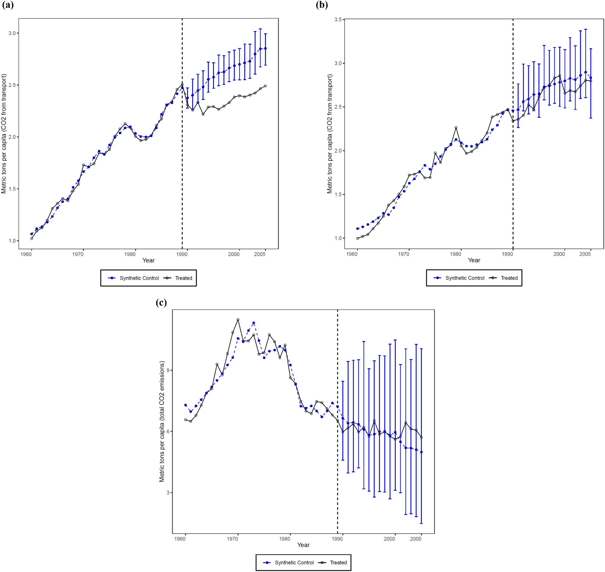
PIs for SCM. (a) Synthetic Sweden (Transport). (b) Synthetic Norway (Transport). (c) Synthetic Sweden (Country-level).
The 95% PIs are built around the predicted potential emission levels for synthetic Sweden and synthetic Norway assuming no carbon taxes. In Figure 9a, the post-treatment per-capita CO2 emissions from transport in Sweden always lie below the PIs for synthetic Sweden. This is evidence that the difference between Sweden and synthetic Sweden is greater than what would be expected from random error.
In Figure 9b, the observed per-capita CO2 emissions from transport in Norway overlap with the PIs of CO2 emissions for synthetic Norway after 1991. This indicates that the differences between Norway and synthetic Norway lie within the range one could reasonably expect from random error, and thus cannot be confidently attributed to the carbon tax.
A similar conclusion holds for total emissions for country-level Sweden as shown in Figure 9c. While scpi produced a somewhat different trajectory for synthetic (country-level) Sweden, and a better fit during the pre-treatment period, the wide PIs mean that we are unable to attribute differences between country-level Sweden and its synthetic counterpart to the carbon tax.
How does scpi reinforce/change my conclusion about the effect of carbon taxes? The answer to this question consists of two parts. Firstly, it further confirms Andersson (2019)’s finding that the Swedish carbon taxes largely reduced CO2 emissions from transport in Sweden. Secondly, when we extend the analysis to Norway’s transport sector and country-level Sweden, we are unable to find corroborating evidence outside of Sweden’s transport sector.
8 Conclusion
Andersson (2019) is one of the few articles that find a large and economically significant effect of carbon taxes on CO2 emissions. For example, in her review, Green (2021) concludes that “[…] the majority of studies suggest that the aggregate reductions from carbon pricing on emissions are limited – generally between 0 and 2% per year.” The unusually large effect size and the high quality of Andersson’s analysis have made his study influential. Thus, it’s interesting to know whether his results are reproducible and reliable and whether his estimated effects can be identified in other settings. To address this, I applied Clemens’s (2017) framework of replication and robustness tests to an analysis of Andersson’s (2019) research.
Table 7 summarizes my main findings. In that table, I apply a five-point scale (5 – Contradicts, 4 – Does Not Support, 3 – Uninformative, 2 – Confirms, 1 – Strongly Confirms) to facilitate the interpretation of my results for the internal and external validity of Andersson’s study.
Summary of key results
| Analysis | Reference | Description | Conclusion/Comment |
|---|---|---|---|
| Swedish Transport Sector | |||
| SCM (VAT + Carbon Tax) | Figure 1a | Use Andersson’s (2019) data and code | 1 – Strongly confirms |
| Identical results to Andersson | |||
| SCM (VAT + Carbon Tax) | Figure 1b | Use Andersson’s (2019) data and code but drop Denmark | 1 – Strongly confirms |
| Very similar results to Andersson | |||
| SCM (VAT + Carbon Tax) | Figure 1b | Use data compiled from original sources with alternative calculation of emissions data | 2 – Confirms |
| Similar results to Andersson but emissions data covers fewer years and is thus less reliable | |||
| Regression (Carbon Tax) | Figure 2a | Use Andersson’s (2019) data and code but drop Denmark | 1 – Strongly confirms |
| Very similar results to Andersson | |||
| Regression (Carbon Tax) | Figure 2b | Estimate gasoline consumption regression using Prais-Winsten | 2 – Confirms |
| Estimated effect approximately half the size of Andersson | |||
| scpi (VAT + Carbon Tax) | Figure 9a | Add PIs to the SCM estimates | 1 – Strongly confirms |
| Very similar results to Andersson | |||
| Norwegian Transport Sector | |||
| SCM (Carbon Tax) | Figure 3b | Uses same predictor variables as Andersson | 4 – Does not support |
| No evidence of an emissions effect | |||
| Regression (Carbon Tax) | Figure 7 | Estimate gasoline consumption regression using Prais-Winsten | 3 – Uninformative |
| The actual regression results strongly support Andersson. However, the estimates are at variance with the SCM estimates and so large as to be implausible. Further, the regression analysis ignores diesel consumption which makes the results suspect | |||
| scpi (Carbon Tax) | Figure 9b | Add PIs to the SCM estimates | 4 – Does not support |
| No evidence of an emissions effect | |||
| Country-Level Sweden | |||
| SCM (Carbon Tax) | Figure 8 | Extends analysis beyond the Swedish transport sector to all of Sweden | 3 – Uninformative |
| SCM analysis fails to produce a reliable counterfactual so the results are uninformative | |||
| scpi (Carbon Tax) | Figure 9c | Add PIs to the SCM estimates | 4 – Uninformative |
| No evidence of an emissions effect | |||
Turning first to Andersson’s direct study of the Swedish transport sector, my results confirm and strongly confirm Andersson’s findings. I both reproduce his results and demonstrate that they are robust to a number of modifications in his analysis. Andersson estimated a combined VAT and carbon tax emission reduction of 10.9% for the Swedish transport sector and attributed a 6.3% reduction to the carbon tax alone. I estimated reductions of 12.9 and 7.7%, respectively. These slightly larger estimates result from omitting carbon-tax adaptor Denmark from the control group to avoid potential bias and applying more advanced techniques to estimate the respective effects of VAT and carbon taxes on gasoline consumption.
The one relatively minor discrepancy with Andersson that I found is that using the Prais-Winsten estimator to estimate gasoline consumption in the face of serial correlation produced price and tax effects approximately half of what Andersson found. However, Andersson (and I) consider results based on regression analysis of gasoline demand to be less reliable than those using synthetic control counterfactuals. As a result, I do not interpret my results from Prais-Winsten estimator as weakening Andersson’s conclusions for the Swedish transport sector.
This was not the case when I extended Andersson’s analysis to estimating the effect of carbon taxes on emissions in the Norwegian transport sector. I found a relatively small (2.4%) emissions reduction effect. Moreover, for several years during the post-treatment period (1996–1999), emissions for the Norwegian transport industry actually exceeded that of its synthetic control counterfactual assuming no carbon tax. Further, even the small differences that were observed lay within the range of values one might reasonably expect from random error. Thus, my effort to find corroborating evidence of the effectiveness of the carbon tax in Norway’s transport sector was not successful.
I also attempted to extend Andersson’s analysis to country-level emissions for Sweden. Unfortunately, the pre-treatment fit of synthetic Sweden was sufficiently poor to render this analysis uninformative. Further, when I re-estimated the synthetic control model using recent methods to estimate PIs, I found no evidence of an effect, and the observed differences all lay well inside the PIs. Thus, my effort to find corroborating evidence for country-level Sweden was also unsuccessful.
While pricing the carbon content of fossil fuels can theoretically reduce the consumption of fossil fuels and mitigate CO2 emissions, my analysis demonstrates that the success of such policies varies case by case. I confirm Andersson’s analysis that the Swedish transport sector experienced an immediate drop and a subsequent stable trend in CO2 emissions after the introduction of the carbon tax. However, a similar outcome was not observed for the Norwegian transport sector, nor was the effect discernible for country-level emissions in Sweden. This serves as a cautionary reminder that one should be careful about extending the analyses of one region or sector or time period to other places and times.
Acknowledgements
I gratefully acknowledge the data provided by Julius J. Andersson and Dermot Gately and the helpful advice from my supervisors Tom Coupé and W. Robert Reed. I especially want to express my appreciation to Professor Reed for his invaluable editorial assistance. I am also grateful for the reviewer’s valuable comments that improved the manuscript.
-
Funding information: The author states no funding is involved.
-
Author contributions: The author confirms the sole responsibility for the conception of the study, presented results, and manuscript preparation.
-
Conflict of interest: The author states no conflict of interest.
-
Data availability statement: All the data and codes needed to generate the results in this articles are posted at https://osf.io/x2d6a/.
-
Article note: As part of the open assessment, reviews and the original submission are available as supplementary files on our website.
References
American Economic Association. (2022). The 2022 AEJ Best Paper Awards Have Been Announced. https://www.aeaweb.org/news/2022-aej-best-papers.Suche in Google Scholar
Abadie, A. (2021). Using synthetic controls: Feasibility, data requirements, and methodological aspects. Journal of Economic Literature, 59(2), 391–425.Suche in Google Scholar
Abadie, A., & Gardeazabal, J. (2003). The economic costs of conflict: A case study of the Basque Country. American Economic Review, 93(1), 113–132.Suche in Google Scholar
Abadie, A., Diamond, A., & Hainmueller, J. (2010). Synthetic control methods for comparative case studies: Estimating the effect of California’s tobacco control program. Journal of the American Statistical Association, 105(490), 493–505.Suche in Google Scholar
Abadie, A., Diamond, A., & Hainmueller, J. (2011). Synth: An R package for synthetic control methods in comparative case studies. Journal of Statistical Software, 42(13), 1–17.Suche in Google Scholar
Andersen, M. S., Dengsøe, N., & Pedersen, A. B. (2001). An evaluation of the impact of green taxes in the Nordic countries. Nordic Council of Ministers.Suche in Google Scholar
Andersson, J. J. (2019). Carbon taxes and CO2 emissions: Sweden as a case study. American Economic Journal: Economic Policy, 11(4), 1–30.Suche in Google Scholar
Bonander, C., Humphreys, D., & Degli Esposti, M. (2021). Synthetic control methods for the evaluation of single-unit interventions in epidemiology: A tutorial. American Journal of Epidemiology, 190(12), 2700–2711.Suche in Google Scholar
Bonander, C., Jakobsson, N., & Johansson, N. (2023). Reproduction and replication analyses of Andersson (2019): A replication report from the Toronto Replication Games. (No. 26). I4R Discussion Paper Series.Suche in Google Scholar
Bottomley, C., Ooko, M., Gasparrini, A., & Keogh, R. (2023). In praise of Prais‐Winsten: An evaluation of methods used to account for autocorrelation in interrupted time series. Statistics in Medicine, 42(8), 1277–1288.Suche in Google Scholar
Bruvoll, A., & Larsen, B. M. (2004). Greenhouse gas emissions in Norway: Do carbon taxes work? Energy Policy, 32(4), 493–505.Suche in Google Scholar
Cattaneo, M. D., Feng, Y., & Titiunik, R. (2021). Prediction intervals for synthetic control methods. Journal of the American Statistical Association, 116(536), 1865–1880.Suche in Google Scholar
Cattaneo, M. D., Feng, Y., Palomba, F., & Titiunik, R. (2022). scpi: Uncertainty quantification for synthetic control methods. arXiv preprint arXiv:2202.05984.Suche in Google Scholar
Clemens, M. A. (2017). The meaning of failed replications: A review and proposal. Journal of Economic Surveys, 31(1), 326–342.Suche in Google Scholar
Davis, L. W., & Kilian, L. (2011). Estimating the effect of a gasoline tax on carbon emissions. Journal of Applied Econometrics, 26(7), 1187–1214.Suche in Google Scholar
Duvendack, M., Palmer-Jones, R. W., & Reed, W. R. (2015). Replications in economics: A progress report. Econ Journal Watch, 12(2), 164–191.Suche in Google Scholar
Enevoldsen, M. K., Ryelund, A. V., & Andersen, M. S. (2007). Decoupling of industrial energy consumption and CO2-emissions in energy-intensive industries in Scandinavia. Energy Economics, 29(4), 665–692.Suche in Google Scholar
European Commission. (2023). Carbon leakage. https://climate.ec.europa.eu/eu-action/eu-emissions-trading-system-eu-ets/free-allocation/carbon-leakage_en.Suche in Google Scholar
Green, J. F. (2021). Does carbon pricing reduce emissions? A review of ex-post analyses. Environmental Research Letters, 16(4), 043004.Suche in Google Scholar
IEA. (2009). Energy Prices and Taxes, First Quarter 2009. https://www.oecd-ilibrary.org/energy/energy-prices-and-taxes/volume-2009/issue-1_energy_tax-v2009-1-en.Suche in Google Scholar
IEA. (2019). Energy policies of IEA Countries: Sweden 2019 Review. https://webstore.iea.org/energy-policies-of-iea-countries-sweden-2019-review.Suche in Google Scholar
Kaul, A., Klößner, S., Pfeifer, G., & Schieler, M. (2015). Synthetic control methods: Never use all pre-intervention outcomes together with covariates. MPRA Paper, 83790.Suche in Google Scholar
Li, S., Linn, J., & Muehlegger, E. (2014). Gasoline taxes and consumer behavior. American Economic Journal: Economic Policy, 6(4), 302–342.Suche in Google Scholar
Lin, B., & Li, X. (2011). The effect of carbon tax on per capita CO2 emissions. Energy Policy, 39(9), 5137–5146.Suche in Google Scholar
Metcalf, G. E. (2019). On the economics of a carbon tax for the United States. Brookings Papers on Economic Activity, 2019(1), 405–484.Suche in Google Scholar
Metcalf, G. E. (2021). Carbon taxes in theory and practice. Annual Review of Resource Economics, 13, 245–265.Suche in Google Scholar
Mueller-Langer, F., Fecher, B., Harhoff, D., & Wagner, G. G. (2019). Replication studies in economics – How many and which papers are chosen for replication, and why? Research Policy, 48(1), 62–83.Suche in Google Scholar
Natural Resources Canada. (2014). Learn the fact: Fuel consumption and CO2. https://natural-resources.canada.ca/sites/www.nrcan.gc.ca/files/oee/pdf/transportation/fuel-efficient-technologies/autosmart_factsheet_6_e.pdf.Suche in Google Scholar
Pretis, F. (2022). Does a carbon tax reduce CO2 emissions? Evidence from British Columbia. Environmental and Resource Economics, 83(1), 115–144.Suche in Google Scholar
Rivers, N., & Schaufele, B. (2015). Salience of carbon taxes in the gasoline market. Journal of Environmental Economics and Management, 74, 23–36. doi: 10.1016/j.jeem.2015.07.002.Suche in Google Scholar
Samuel, J., Ydstedt, A., & Asen, E. (2020). Looking back on 30 years of carbon taxes in Sweden. Fiscal fact, 727. Suche in Google Scholar
Statens, F. (2003). Greenhouse gas emissions in Norway 1990–2001. Norway: National Inventory Report 2003.Suche in Google Scholar
Tirkaso, W. T., & Gren, M. (2020). Road fuel demand and regional effects of carbon taxes in Sweden. Energy Policy, 144, 111648.Suche in Google Scholar
© 2024 the author(s), published by De Gruyter
This work is licensed under the Creative Commons Attribution 4.0 International License.
Artikel in diesem Heft
- Regular Articles
- Political Turnover and Public Health Provision in Brazilian Municipalities
- Examining the Effects of Trade Liberalisation Using a Gravity Model Approach
- Operating Efficiency in the Capital-Intensive Semiconductor Industry: A Nonparametric Frontier Approach
- Does Health Insurance Boost Subjective Well-being? Examining the Link in China through a National Survey
- An Intelligent Approach for Predicting Stock Market Movements in Emerging Markets Using Optimized Technical Indicators and Neural Networks
- Analysis of the Effect of Digital Financial Inclusion in Promoting Inclusive Growth: Mechanism and Statistical Verification
- Effective Tax Rates and Firm Size under Turnover Tax: Evidence from a Natural Experiment on SMEs
- Re-investigating the Impact of Economic Growth, Energy Consumption, Financial Development, Institutional Quality, and Globalization on Environmental Degradation in OECD Countries
- A Compliance Return Method to Evaluate Different Approaches to Implementing Regulations: The Example of Food Hygiene Standards
- Panel Technical Efficiency of Korean Companies in the Energy Sector based on Digital Capabilities
- Time-varying Investment Dynamics in the USA
- Preferences, Institutions, and Policy Makers: The Case of the New Institutionalization of Science, Technology, and Innovation Governance in Colombia
- The Impact of Geographic Factors on Credit Risk: A Study of Chinese Commercial Banks
- The Heterogeneous Effect and Transmission Paths of Air Pollution on Housing Prices: Evidence from 30 Large- and Medium-Sized Cities in China
- Analysis of Demographic Variables Affecting Digital Citizenship in Turkey
- Green Finance, Environmental Regulations, and Green Technologies in China: Implications for Achieving Green Economic Recovery
- Coupled and Coordinated Development of Economic Growth and Green Sustainability in a Manufacturing Enterprise under the Context of Dual Carbon Goals: Carbon Peaking and Carbon Neutrality
- Revealing the New Nexus in Urban Unemployment Dynamics: The Relationship between Institutional Variables and Long-Term Unemployment in Colombia
- The Roles of the Terms of Trade and the Real Exchange Rate in the Current Account Balance
- Cleaner Production: Analysis of the Role and Path of Green Finance in Controlling Agricultural Nonpoint Source Pollution
- The Research on the Impact of Regional Trade Network Relationships on Value Chain Resilience in China’s Service Industry
- Social Support and Suicidal Ideation among Children of Cross-Border Married Couples
- Asymmetrical Monetary Relations and Involuntary Unemployment in a General Equilibrium Model
- Job Crafting among Airport Security: The Role of Organizational Support, Work Engagement and Social Courage
- Does the Adjustment of Industrial Structure Restrain the Income Gap between Urban and Rural Areas
- Optimizing Emergency Logistics Centre Locations: A Multi-Objective Robust Model
- Geopolitical Risks and Stock Market Volatility in the SAARC Region
- Trade Globalization, Overseas Investment, and Tax Revenue Growth in Sub-Saharan Africa
- Can Government Expenditure Improve the Efficiency of Institutional Elderly-Care Service? – Take Wuhan as an Example
- Media Tone and Earnings Management before the Earnings Announcement: Evidence from China
- Review Articles
- Economic Growth in the Age of Ubiquitous Threats: How Global Risks are Reshaping Growth Theory
- Efficiency Measurement in Healthcare: The Foundations, Variables, and Models – A Narrative Literature Review
- Rethinking the Theoretical Foundation of Economics I: The Multilevel Paradigm
- Financial Literacy as Part of Empowerment Education for Later Life: A Spectrum of Perspectives, Challenges and Implications for Individuals, Educators and Policymakers in the Modern Digital Economy
- Special Issue: Economic Implications of Management and Entrepreneurship - Part II
- Ethnic Entrepreneurship: A Qualitative Study on Entrepreneurial Tendency of Meskhetian Turks Living in the USA in the Context of the Interactive Model
- Bridging Brand Parity with Insights Regarding Consumer Behavior
- The Effect of Green Human Resources Management Practices on Corporate Sustainability from the Perspective of Employees
- Special Issue: Shapes of Performance Evaluation in Economics and Management Decision - Part II
- High-Quality Development of Sports Competition Performance Industry in Chengdu-Chongqing Region Based on Performance Evaluation Theory
- Analysis of Multi-Factor Dynamic Coupling and Government Intervention Level for Urbanization in China: Evidence from the Yangtze River Economic Belt
- The Impact of Environmental Regulation on Technological Innovation of Enterprises: Based on Empirical Evidences of the Implementation of Pollution Charges in China
- Environmental Social Responsibility, Local Environmental Protection Strategy, and Corporate Financial Performance – Empirical Evidence from Heavy Pollution Industry
- The Relationship Between Stock Performance and Money Supply Based on VAR Model in the Context of E-commerce
- A Novel Approach for the Assessment of Logistics Performance Index of EU Countries
- The Decision Behaviour Evaluation of Interrelationships among Personality, Transformational Leadership, Leadership Self-Efficacy, and Commitment for E-Commerce Administrative Managers
- Role of Cultural Factors on Entrepreneurship Across the Diverse Economic Stages: Insights from GEM and GLOBE Data
- Performance Evaluation of Economic Relocation Effect for Environmental Non-Governmental Organizations: Evidence from China
- Functional Analysis of English Carriers and Related Resources of Cultural Communication in Internet Media
- The Influences of Multi-Level Environmental Regulations on Firm Performance in China
- Exploring the Ethnic Cultural Integration Path of Immigrant Communities Based on Ethnic Inter-Embedding
- Analysis of a New Model of Economic Growth in Renewable Energy for Green Computing
- An Empirical Examination of Aging’s Ramifications on Large-scale Agriculture: China’s Perspective
- The Impact of Firm Digital Transformation on Environmental, Social, and Governance Performance: Evidence from China
- Accounting Comparability and Labor Productivity: Evidence from China’s A-Share Listed Firms
- An Empirical Study on the Impact of Tariff Reduction on China’s Textile Industry under the Background of RCEP
- Top Executives’ Overseas Background on Corporate Green Innovation Output: The Mediating Role of Risk Preference
- Neutrosophic Inventory Management: A Cost-Effective Approach
- Mechanism Analysis and Response of Digital Financial Inclusion to Labor Economy based on ANN and Contribution Analysis
- Asset Pricing and Portfolio Investment Management Using Machine Learning: Research Trend Analysis Using Scientometrics
- User-centric Smart City Services for People with Disabilities and the Elderly: A UN SDG Framework Approach
- Research on the Problems and Institutional Optimization Strategies of Rural Collective Economic Organization Governance
- The Impact of the Global Minimum Tax Reform on China and Its Countermeasures
- Sustainable Development of Low-Carbon Supply Chain Economy based on the Internet of Things and Environmental Responsibility
- Measurement of Higher Education Competitiveness Level and Regional Disparities in China from the Perspective of Sustainable Development
- Payment Clearing and Regional Economy Development Based on Panel Data of Sichuan Province
- Coordinated Regional Economic Development: A Study of the Relationship Between Regional Policies and Business Performance
- A Novel Perspective on Prioritizing Investment Projects under Future Uncertainty: Integrating Robustness Analysis with the Net Present Value Model
- Research on Measurement of Manufacturing Industry Chain Resilience Based on Index Contribution Model Driven by Digital Economy
- Special Issue: AEEFI 2023
- Portfolio Allocation, Risk Aversion, and Digital Literacy Among the European Elderly
- Exploring the Heterogeneous Impact of Trade Agreements on Trade: Depth Matters
- Import, Productivity, and Export Performances
- Government Expenditure, Education, and Productivity in the European Union: Effects on Economic Growth
- Replication Study
- Carbon Taxes and CO2 Emissions: A Replication of Andersson (American Economic Journal: Economic Policy, 2019)