Higher-order circular intuitionistic fuzzy time series forecasting methodology: Application of stock change index
-
Shahzaib Ashraf
 und
Choonkil Park
und
Choonkil Park

Abstract
This article presents a higher-order circular intuitionistic fuzzy time series forecasting method for predicting the stock change index, which is shown to be an improvement over traditional time series forecasting methods. The method is based on the principles of circular intuitionistic fuzzy set theory. It uses both positive and negative membership values and a circular radius to handle uncertainty and imprecision in the data. The circularity of the time series is also taken into consideration, leading to more accurate and robust forecasts. The higher-order forecasting capability of this method provides more comprehensive predictions compared to previous methods. One of the key challenges we face when using the amount featured as a case study in our article to project the future value of ratings is the influence of the stock market index. Through rigorous experiments and comparison with traditional time series forecasting methods, the results of the study demonstrate that the proposed higher-order circular intuitionistic fuzzy time series forecasting method is a superior approach for predicting the stock change index.
1 Introduction
Decision-making can be defined as the process of selecting the best option from a collection of options based on a range of factors to achieve organizational goals [1]. The main research area in the complex decision-making problem of today, with several goals or circumstances, is multi-criteria decision making (MCDM). A number of MCDM techniques, such as printer selection [2], solar power plant [3], and others, have been developed to address decisions involving a range of conflicting criteria in ambiguous situations. These classic MCDM algorithms cannot handle ambiguous or inaccurate language judgments since precise numerical values are required. To better capture this ambiguity, intuitionistic fuzzy sets, neutrosophic sets, and spherical fuzzy sets (SFSs) [4] have been added to standard fuzzy sets in MCDM techniques. In this article, a proposed method is used to forecast the data, which will be helpful for MCDM in the future. Fuzzy set theory is one of the most impressive tools for addressing the problems of handling accurate and sufficient data for real-world decision-making due to the confusion of statistics. Zadeh created a fuzzy set to support her in decision-making when faced with challenges in daily life [5]. There is only one element with a membership degree that varies from 0 to 1 for each domain set component
Because they deal with situations that comprise particular attributes in which the sum of their membership and nonmembership degrees is greater than one, according to several real-life choice concepts. IFS would not be able to produce an appropriate outcome in this situation. The Pythagorean fuzzy set (PyFS) was recommended by Yager [11] as a solution to these problems. In a PyFS, the degree of membership of an element is determined by the Pythagorean theorem, which relates the length of the sides of a right triangle to the length of its hypotenuse. This allows for a more nuanced representation of uncertainty than traditional fuzzy sets, which only allow for binary membership values of either 0 or 1. We now want to determine the neutral membership independently. Cuong and Kreinovich [12] expressed the concept of a picture fuzzy set (PFS). He used three items with the limitation of PFS membership degree
Making predictions about upcoming events or patterns based on historical data and knowledge is the process of predicting. It is used in a variety of fields, including finance, economics, marketing, and weather prediction, among others. To solve problems that changed over time, the time series data technique was used. Song and Chissom’s definition of time series in fuzzy time series [20] outlines the notion of fuzzy time series data or its techniques. Using fuzzy sets, Song and Chissom [21,22] projected the data. Following this, Kumar and Gangwar modify the Song and Chissom’s method [23]. To estimate data in fuzzy theory, many scholars employ diverse strategies. The majority of them made use of IFSs. Kumar and Gangwar [24] and Joshi and Kumar [25] used IFSs to include the amount of uncertainty in fuzzy logical links and develop only a few temporal forecasting models [26]. Jiang et al. [27] derived the formula used to predict wind speed. Prior to this, the majority of the researchers used his proposed approach using data from the University of Alabama [28,29]. They compared the mistakes of each result with one another after determining the conclusion to determine the best planned technique.
There are several different definitions of fuzzy forecasting that have been proposed by researchers. Some of these include:
Linguistic Forecasting: This definition views fuzzy forecasting as a method that uses linguistic variables to express uncertainty in the forecast. Linguistic variables are variables that can take on values from a predefined set of linguistic terms, such as “high,” “medium,” and “low” [30].
Probabilistic Forecasting: This definition views fuzzy forecasting as a method that uses fuzzy sets to express the probability of events. Fuzzy sets are sets that allow for partial membership, meaning that an element can belong to a set to a certain degree [31].
Interval Forecasting: This definition views fuzzy forecasting as a method that uses fuzzy intervals to express the uncertainty in the forecast. Fuzzy intervals are intervals that allow for partial membership, meaning that an element can belong to an interval to a certain degree [32].
Hybrid Forecasting: This definition views fuzzy forecasting as a method that combines different forecasting techniques, such as regression analysis and time series analysis, with fuzzy set theory [33].
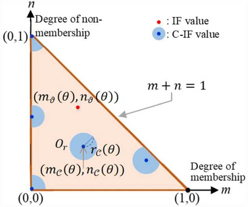
Graphical representation of C-IFSs.
Scientists used to make choices by rating and evaluating data. However, they are insufficient to estimate future values. Chen [38] began by using time series analysis to forecast enrollments. Kumar and Gangwar [39] proposed attempting to cope with forecasting by employing induced IFSs. Abhishekh et al. [40] employed this strategy on higher-order IFSs. Furthermore, if we want to check the radius of a circle in IFS, we are unable to find it. As a result, authors are thrilled to be able to meet this need. As a result, we must employ C-IFS to deal with this sort of issue. This is a transition to all predicting algorithms capable of handling any form of membership, and nonmembership includes circular radius. They are useful when we need to calculate the radius of IFS. The question arises: Why do we calculate the radius of any set? The answer is that after finding the radius, we know to check where the values of oversetting lie in this radius, which is helpful in observing our results. Hence, we implicate this technique in this article to solve any type of data for future prediction. IFS cannot handle this type of thing. We worked on filling this with circular intuitionistic fuzzy time series (C-IFTSs), which are useful for time series forecasting, particularly when the total of membership and nonmembership is less than or equal to one with a circular radius. We offer a forecasting strategy for higher-order C-IFTSs that has lower error rates than earlier studies in this work. As part of my proposed strategy, we used the example of the stock change index. The motivation for researching stock change indices is likely to be to better understand the dynamics of financial markets and to provide investors with useful information for making informed investment decisions. Stock change indices track the performance of a group of stocks and can serve as a barometer for the overall health of a given market or economy. By analyzing changes in these indices over time, researchers can gain insights into market trends, investor sentiment, and other factors that drive stock prices. In addition, the results of such research can inform investment strategies and help investors make more informed decisions about buying, holding, or selling stocks. This idea may be applied to a range of potential future predictions.
The rest of this article is organized as follows:
C-IFS and fuzzy sets are stated as being utilized to connect the other portions of the article.
Following that, we gave some definitions for implementing my proposed technique, as well as a circular intuitionistic membership, nonmembership, and radius number for determining the score value.
Time-variant and time-invariant C-IFTSs concepts were provided.
Following that, we showed a flowchart outlining how we would anticipate data using our suggested technique, as well as specific descriptions of the proposed method.
To evaluate the outcomes, we applied this approach to the stock change index and computed the findings on tables.
After that, we expanded on this work to a higher-order forecasting.
Finally, we presented the article’s conclusion.
2 Preliminaries
This section provides concise definitions of fuzzy sets, circular fuzzy sets, and time series analysis. They are important for linking to the following portion of this article.
Definition 2.1
The fuzzy set notion introduced by Zadeh is stated as follows: Let
where
Definition 2.2
[41] Suppose a nonempty set
Definition 2.3
[42] Let
where
and
The level of uncertainty is calculated as follows:
Definition 2.4
[43] The following is a definition of the operations that C-IFS entails. For every
- (3)(4)
Definition 2.5
[44] Let
Theorem 2.6
For any
Proof
We must demonstrate that the formulas mentioned in expression (4) abide by the property of metric [45]. As previously demonstrated, the terms indicated in (3) are well-defined distances in IFS
Because it is clear from the definition of C-IFSs,
Because
holds.
We know that distance without radius.
holds for the IFSs
From well-known inequality
for all choices of ,
Definition 2.7
If
Definition 2.8
If circular intuitionistic logical relationship exist
Definition 2.9
Suppose
Definition 2.10
Suppose
3 An algorithm of handling circular intuitionistic time series forecasting
There are three parts to our algorithm (A, B, and C). To cope with situations of this nature in C-IFTSs, we created a strategy. The first portion establishes the C-ILR and its groups; the second section employs the circular intuitionistic forecasting technique to determine the forecasted value of our issue; and the last section informs us of the approach’s flaws. Figure 2 shows the flow chart of the proposed technique.

A flowchart that shows how the proposed method works.
A. First-order C-IFTSs proposed method of forecasting The following will guide you through all the procedures necessary to establish a C-ILR and its groups using the score formula.
Step I: The universe of discourse is determined by time series data to the stated range
Step II: A subset of
Step III: Compute the
Step IV: Calculate the radius of a circular intuitionistic fuzzy set by using equations (10) and (11).
In an IFS
where
The radius of the
Step V: To calculate the score degree, utilize the following equation, and then choose the score degree that has the highest possible value [46]:
Step VI: Construct the circular intuitionistic fuzzy logical relationships (C-IFLRs): If
Step VII: Depending on the C-IFLRs, create circular intuitionistic fuzzy logical relationship groups (C-IFLRGs).
B. Measure the forecasted value of circular intuitionistic fuzzy sets
The following is the technique that is used to determine the predicted values:
If circular intuitionistic value of data
If C-IFLRGs of
If C-IFLRGs of
If C-IFLRGs of
C. Measurement of error by using root mean square error (RMSE) and average forecasting error (AFE)
Techniques such as RMSE and AFE are utilized rather frequently to evaluate the precision of time series forecasting. The following definitions are applicable to all types of error measures.
Forecasting percentage error (fpe)
In this case, the predicted and observed data of the time series are denoted by
4 Case study
The values of specific shares are used to derive a stock market index, which is a measurement of the worth of a portion of the stock market. This value is computed based on the index. It is a technique that investors employ to provide a description of the market and to compare the returns generated by various investments. An index provides a fast assessment of a market’s condition. Active funds are a reduced method of investing that offers greater returns than most fund managers and aids investors in more consistently achieving their objectives. In this article, we picked the data from the stock change index (Taiwan).
Forecasting the change in the Taiwan stock exchange index can bring several benefits for investors and traders. Some of these benefits include:
Improved decision-making: By having an accurate forecast, investors and traders can make informed decisions on when to buy or sell their investments, which can lead to better returns.
Risk management: Accurate forecasting can help investors and traders manage their risk by allowing them to make informed decisions on when to enter or exit the market.
Increased confidence: With a better understanding of the future progress of the stock change index, investors and traders can have increased confidence in their investment decisions, which can help them make more informed and profitable trades.
Improved portfolio diversification: By forecasting the stock change index, investors and traders can better understand the potential impact of their investments on their overall portfolio, which can help them diversify their investments for better risk management.
4.1 Implementation of the proposed method of stock change index
It is important to note that stock market forecasts are not always accurate and that past performance does not guarantee future results. Therefore, investors and traders should always use a combination of forecasting tools and fundamental analysis when making investment decisions.
We apply the method using data from the stock index in 2001 and explain the findings step-by-step to make the process of understanding and verifying the suggested model as simple as possible. The following is a list of the steps:
Step I : The universe of discourse
Universe of discourse
Fuzzy stock change index
| Date | True value | C-Intuitionistic value | Date | True value | C-Intuitionistic value |
|---|---|---|---|---|---|
| 01-11-2001 | 3929.69 |
|
03-12-2001 | 4646.61 |
|
| 02-11-2001 | 3998.48 |
|
04-12-2001 | 4766.43 |
|
| 05-11-2001 | 4080.51 |
|
05-12-2001 | 4924.56 |
|
| 06-11-2001 | 4082.92 |
|
06-12-2001 | 5208.86 |
|
| 07-11-2001 | 4158.15 |
|
07-12-2001 | 5333.93 |
|
| 08-11-2001 | 4135.03 |
|
10-12-2001 | 5321.28 |
|
| 09-11-2001 | 4123.78 |
|
11-12-2001 | 5273.97 |
|
| 12-11-2001 | 4172.63 |
|
12-12-2001 | 5539.31 |
|
| 13-11-2001 | 4136.54 |
|
13-12-2001 | 5407.54 |
|
| 14-11-2001 | 4277.70 |
|
14-12-2001 | 5486.73 |
|
| 15-11-2001 | 4403.59 |
|
17-12-2001 | 5456.15 |
|
| 16-11-2001 | 4446.62 |
|
18-12-2001 | 5329.19 |
|
| 19-11-2001 | 4548.63 |
|
19-12-2001 | 5221.96 |
|
| 20-11-2001 | 4455.80 |
|
20-12-2001 | 5309.10 |
|
| 21-11-2001 | 4533.37 |
|
21-12-2001 | 5109.24 |
|
| 22-11-2001 | 4450.02 |
|
24-12-2001 | 5164.73 |
|
| 23-11-2001 | 4519.08 |
|
25-12-2001 | 5372.81 |
|
| 26-11-2001 | 4608.32 |
|
26-12-2001 | 5392.43 |
|
| 27-11-2001 | 4580.33 |
|
27-12-2001 | 5332.98 |
|
| 28-11-2001 | 4447.58 |
|
28-12-2001 | 5398.28 |
|
| 29-11-2001 | 4465.83 |
|
31-12-2001 | 5551.24 |
|
| 30-11-2001 | 4441.12 |
|
Step II: The universe of discourse is divided into 14 intervals by
Step III: Following 14 C-IFTS,
By using equations (8) and (9), the grades of membership and nonmembership in circular intuitionistic fuzzy sets are calculated as follows: Suppose
Step IV: Calculate the radius of circular intuitionistic fuzzy set by using equations (10) and (11).
Step V: Use (12) in your computation to obtain the C-IFS score value.
The actual value of 4080.51 is between the two values of the circular intuitionistic membership and nonmembership of
Similarly,
We must calculate the degree of score 4080.51
So the degree of score 4080.51 in
Step VI: Circular intuitionistic logical relationships are in presented Table 2.
Circular intuitionistic logical relationships of order I
|
|
|
|
|
|
|
|
|
|
|
|
|
|
|
|
|
|
|
|
|
|
|
|
|
|
|
|
|
|
|
|
|
|
|
|
|
|
|
|
|
|
|
|
|
|
|
|
Step VII: We developed a collection of C-IFLRGs based on C-IFLRs, which are presented in Table 3.
Circular intuitionistic logical relationship groups of order I
|
|
|
|
|
|||||
|
|
|
|
|
|
||||
|
|
||||||||
|
|
|
|
|
|
|
|||
|
|
|
|
|
|||||
|
|
|
|
||||||
|
|
||||||||
|
|
||||||||
|
|
|
|||||||
|
|
|
|
||||||
|
|
|
|
|
|
|
|
|
|
|
|
|
|
B. Measure the forecasted value of circular intuitionistic fuzzy sets
The computed forecasted values are shown in Table 4. We are unable to predict what the anticipated value for November 1, 2001, will be since we do not have access to the beginning value for that day. The estimated value for the next day was computed similarly.
Forecasted value of stock change index of order I
| Date | True value | Forecasted value | Years | True value | Forecasted value |
|---|---|---|---|---|---|
| 01-11-2001 | 3929.69 | — | 03-12-2001 | 4646.61 | 4,520 |
| 02-11-2001 | 3998.48 | 4,100 | 04-12-2001 | 4766.43 | 4,600 |
| 05-11-2001 | 4080.51 | 4,100 | 05-12-2001 | 4924.56 | 4,880 |
| 06-11-2001 | 4082.92 | 4,100 | 06-12-2001 | 5208.86 | 5,240 |
| 07-11-2001 | 4158.15 | 4,100 | 07-12-2001 | 5333.93 | 5,360 |
| 08-11-2001 | 4135.03 | 4,220 | 10-12-2001 | 5321.28 | 5,420 |
| 09-11-2001 | 4123.78 | 4,220 | 11-12-2001 | 5273.97 | 5,420 |
| 12-11-2001 | 4172.63 | 4,220 | 12-12-2001 | 5539.31 | 5,420 |
| 13-11-2001 | 4136.54 | 4,220 | 13-12-2001 | 5407.54 | 5,420 |
| 14-11-2001 | 4277.70 | 4,220 | 14-12-2001 | 5486.73 | 5,420 |
| 15-11-2001 | 4403.59 | 4,400 | 17-12-2001 | 5456.15 | 5,420 |
| 16-11-2001 | 4446.62 | 4,520 | 18-12-2001 | 5329.19 | 5,420 |
| 19-11-2001 | 4548.63 | 4,520 | 19-12-2001 | 5221.96 | 5,420 |
| 20-11-2001 | 4455.80 | 4,520 | 20-12-2001 | 5309.10 | 5,420 |
| 21-11-2001 | 4533.37 | 4,520 | 21-12-2001 | 5109.24 | 5,420 |
| 22-11-2001 | 4450.02 | 4,520 | 24-12-2001 | 5164.73 | 5,240 |
| 23-11-2001 | 4519.08 | 4,520 | 25-12-2001 | 5372.81 | 5,240 |
| 26-11-2001 | 4608.32 | 4,520 | 26-12-2001 | 5392.43 | 5,420 |
| 27-11-2001 | 4580.33 | 4,600 | 27-12-2001 | 5332.98 | 5,420 |
| 28-11-2001 | 4447.58 | 4,600 | 28-12-2001 | 5398.28 | 5,420 |
| 29-11-2001 | 4465.83 | 4,520 | 31-12-2001 | 5551.24 | 5,420 |
| 30-11-2001 | 4441.12 | 4,520 |
Figure 3 presents a graph that illustrates the true value as well as the observed value that make up the stock change index.

True value and observed value of order I.
4.2 Circular intuitionistic logical relationship of order II
Now we will compute the circular intuitionistic logical relationship and its groups according to the provided approach to order II stock change index.
The circular intuitionistic logic relations of order II are in Table 5. Table 6 displays the circular intuitionistic logic relation groups that we created based on C-ILRs. These C-ILRs are of order II.
Circular intuitionistic logical relationship of order II
|
|
|
|
|
|
|
|
|
|
|
|
|
|
|
|
|
|
|
|
|
|
|
|
|
|
|
|
|
|
|
|
|
|
|
|
|
|
|
|
|
|
|
|
|
|
|
|
Circular intuitionistic logical relationship groups of order II
|
|
|
|
|
|||
|
|
|
|
|
|
||
|
|
|
|||||
|
|
|
|
|
|
|
|
|
|
|
|||||
|
|
|
|||||
|
|
|
|||||
|
|
|
|
||||
|
|
|
|
|
|
|
|
|
|
|
|
||||
|
|
|
|||||
|
|
|
|||||
|
|
B. Measure the forecasted value of circular intuitionistic fuzzy sets.
Table 7 presents the results of the forecasting calculations that were performed with the help of the defuzzified criteria described in Section B. Figure 4 is a graph that depicts the true value, as well as the observed value, of the stock change index for order II.
Forecasted value of stock change index of order II
| Date | True value | Forecasted value | Years | True value | Forecasted value |
|---|---|---|---|---|---|
| 01-11-2001 | 3929.69 | — | 03-12-2001 | 4646.61 | 4,580 |
| 02-11-2001 | 3998.48 | — | 04-12-2001 | 4766.43 | 4,760 |
| 05-11-2001 | 4080.51 | 4,100 | 05-12-2001 | 4924.56 | 4,880 |
| 06-11-2001 | 4082.92 | 4,100 | 06-12-2001 | 5208.86 | 5,240 |
| 07-11-2001 | 4158.15 | 4,100 | 07-12-2001 | 5333.93 | 5,360 |
| 08-11-2001 | 4135.03 | 4,160 | 10-12-2001 | 5321.2 | 5,240 |
| 09-11-2001 | 4123.78 | 4,220 | 11-12-2001 | 5273.97 | 5,400 |
| 12-11-2001 | 4172.63 | 4,220 | 12-12-2001 | 5539.31 | 5,420 |
| 13-11-2001 | 4136.54 | 4,220 | 13-12-2001 | 5407.54 | 5,360 |
| 14-11-2001 | 4277.70 | 4,220 | 14-12-2001 | 5486.73 | 5,360 |
| 15-11-2001 | 4403.59 | 4,400 | 17-12-2001 | 5456.15 | 5,480 |
| 16-11-2001 | 4446.62 | 4,400 | 18-12-2001 | 5329.19 | 5,360 |
| 19-11-2001 | 4548.63 | 4,520 | 19-12-2001 | 5221.96 | 5,360 |
| 20-11-2001 | 4455.80 | 4,520 | 20-12-2001 | 5309.10 | 5,420 |
| 21-11-2001 | 4533.37 | 4,580 | 21-12-2001 | 5109.24 | 5,420 |
| 22-11-2001 | 4450.02 | 4,520 | 24-12-2001 | 5164.73 | 5,120 |
| 23-11-2001 | 4519.08 | 4,580 | 25-12-2001 | 5372.81 | 5,360 |
| 26-11-2001 | 4608.32 | 4,520 | 26-12-2001 | 5392.43 | 5,360 |
| 27-11-2001 | 4580.33 | 4,640 | 27-12-2001 | 5332.98 | 5,400 |
| 28-11-2001 | 4447.58 | 4,400 | 28-12-2001 | 5398.28 | 5,400 |
| 29-11-2001 | 4465.83 | 4,520 | 31-12-2001 | 5551.24 | 5,400 |
| 30-11-2001 | 4441.12 | 4,520 |

Graph of the actual and proposed value of order II.
C. Measurement of error by using RMSE and AFE
The formulas for determining errors are provided in Table 8 and are used to calculate RMSE and AFE, respectively. Comparing our results with other forecasting methods using RMSE and AFE can give an indication of the accuracy of your forecast. If the RMSE and AFE values are lower than those of other forecasting methods, it means that the proposed method is more accurate because of the lower error.
5 Discussion
Table 8 shows the difference in predicted performance between first- and second-order C-IFTSs. Compared to first-order C-IFTSs forecasting, second-order C-IFTSs forecasting uses error calculation formulas. When we calculate third-order C-IFTS forecasting, the error of the third order is less than the error of the second. Use the same formula to obtain the
The value of RMSE clearly shows the validity of my proposed algorithm to deal with this kind of problem in future prediction. As we discussed earlier, errors show the accuracy of your method. Researchers use this technique to invest the amount in stock index problems. A proposed algorithm is used to handle all these types of problems in fuzzy logic, in which a radius is also given for membership and nonmembership. In the past, no one could give any algorithm to solve this type of problem where the radius was also given. This algorithm is helpful for dealing with this kind of problem.
Radius tells us where the value of membership and nonmembership lies. The radius in C-IFS is important because it can impact the overall shape and size of the circular fuzzy set, which in turn can affect its ability to represent complex and uncertain information in a flexible and intuitive way.
6 Conclusion
With the circular radius, C-IFS membership and nonmembership degree totals are all equal to one or fewer, and they are rapidly gaining favor. It is obvious that utilizing intuitionistic fuzzy sets cannot address this issue; as a result, we employ C-IFS instead of IFSs if the total of the membership value and degree of the nonmembership value are equal. The suggested C-IFS approach was less complex and more straightforward since it employed a simple scoring formula. We used our method to verify the number of stock change indexes, and now we can forecast our data using the given criteria. In addition, we applied this approach to higher-order predictions and displayed the error, which indicates that higher-order forecasts have fewer errors and are thus more helpful for calculating future values. By using the advised strategy, we came up with a prediction for the next few years. Researchers may provide further solutions to the forecasting process in the future. One potential direction for future research could be to apply C-IFTS to various time series forecasting problems and compare their performance to existing methods.
-
Funding information: The authors received no financial support for the research of this article.
-
Author contributions: All authors have contributed equally to this article.
-
Conflict of interest: The authors declare that they have no conflict of interest regarding the publication of the research article.
-
Ethical approval: This article does not contain any studies with human participants or animals performed by any of the authors.
-
Data availability statement: The data used and analyzed during the current study available from the corresponding author on reasonable request.
References
[1] S. Ashraf, N. Rehman, H. AlSalman, and A. H. Gumaei, A decision-making framework using q-rung orthopair probabilistic hesitant fuzzy rough aggregation information for the drug selection to treat COVID-19, Complexity 2022 (2022), 5556309, https://doi.org/10.1155/2022/5556309. Suche in Google Scholar
[2] F. Kutlu Gündogdu, and S. Ashraf, Some Novel Preference Relations for Picture Fuzzy Sets and Selection of 3-D Printers in Aviation 4.0. In Intelligent and Fuzzy Techniques in Aviation 4.0, vol. 372, Springer, Cham, 2022, https://doi.org/10.1007/978-3-030-75067-112. Suche in Google Scholar
[3] S. Khan, S. Abdullah, S. Ashraf, R. Chinram, and S. Baupradist, Decision support technique based on neutrosophic Yager aggregation operators: Application in solar power plant locations-Ťcase study of Bahawalpur, Pakistan, Math. Probl. Eng. 2020 (2020), 6677676, https://doi.org/10.1155/2020/6677676. Suche in Google Scholar
[4] R. Chinram, S. Ashraf, S. Abdullah, and P. Petchkaew, Decision support technique based on spherical fuzzy Yager aggregation operators and their application in wind power plant locations: a case study of Jhimpir, Pakistan J. Math. 2020 (2020), 8824032, https://doi.org/10.1155/2020/8824032. Suche in Google Scholar
[5] L. A. Zadeh, Fuzzy sets, In Fuzzy sets, fuzzy logic, and fuzzy systems: selected papers by Lotfi A Zadeh, 1996. 10.1142/9789814261302_0021Suche in Google Scholar
[6] K. T Atanassov, Intuitionistic fuzzy sets, In Intuitionistic Fuzzy Sets Physica, Heidelberg, 1999. 10.1007/978-3-7908-1870-3_1Suche in Google Scholar
[7] K. Atanassov, Remark on intuitionistic fuzzy numbers. Notes Intuitionistic Fuzzy Sets 13 (2007), no. 3, 29–32. https://ifigenia.org/images/archive/c/c0/20151019135158!NIFS-13-3-29-32.pdf. Suche in Google Scholar
[8] V. L. G. Nayagam, S. Muralikrishnan, and G. Sivaraman, Multi-criteria decision-making method based on interval-valued intuitionistic fuzzy sets, Expert Syst. Appl. 38 (2011), no. 3, 1464–1467, https://doi.org/10.1016/j.eswa.2010.07.055. Suche in Google Scholar
[9] C. Tan, A multi-criteria interval-valued intuitionistic fuzzy group decision making with Choquet integral-based TOPSIS, Expert Syst. Appl. 38 (2011), no. 4, 3023–3033, https://doi.org/10.1016/j.eswa.2010.08.092. Suche in Google Scholar
[10] Z. Xu, Approaches to multiple attribute group decision making based on intuitionistic fuzzy power aggregation operators, KBS 24 (2011), no. 6, 749–760, https://doi.org/10.1016/j.knosys.2011.01.011. Suche in Google Scholar
[11] R. R. Yager, Pythagorean fuzzy subsets, In 2013 joint IFSA world congress and NAFIPS annual meeting (IFSA/NAFIPS), IEEE, 2013, pp. 57–61, https://doi.org/10.1109/IFSA-NAFIPS.2013.6608375. Suche in Google Scholar
[12] B. C. Cuong and V. Kreinovich, Picture fuzzy sets-a new concept for computational intelligence problems, In 2013 third world congress on information and communication technologies (WICT 2013), IEEE, Hanoi, Vietnam, (2013), pp. 1–6, https://doi.org/10.1109/WICT.2013.7113099. Suche in Google Scholar
[13] H. Garg, Some picture fuzzy aggregation operators and their applications to multicriteria decision-making, Arab. J. Sci. Eng. 42 (2017), no. 12, 5275–5290, https://doi.org/10.1007/s13369-017-2625-9. Suche in Google Scholar
[14] P. Dutta, Medical diagnosis via distance measures on picture fuzzy sets, AMA A, 54 (2017), no. 2, 657–672. Suche in Google Scholar
[15] S. Ashraf, S. Abdullah, T. Mahmood, F. Ghani, and T. Mahmood, Spherical fuzzy sets and their applications in multi-attribute decision making problems, J. Intell. Fuzzy Syst., 36 (2019), no. 3, 2829–2844, https://doi.org/10.3233/JIFS-172009. Suche in Google Scholar
[16] S. Ashraf, S. Abdullah, M. Aslam, M. Qiyas, and M. A. Kutbi, Spherical fuzzy sets and its representation of spherical fuzzy t-norms and t-conorms, J. Intell. Fuzzy Syst. 36 (2019), no. 6, 6089–6102, https://doi.org/10.3233/JIFS-181941. Suche in Google Scholar
[17] T. Mahmood, K. Ullah, Q. Khan, and N. Jan, An approach toward decision-making and medical diagnosis problems using the concept of spherical fuzzy sets, Neural Comput. Appl. 31 (2019), no. 11, 7041–7053, https://doi.org/10.1007/s00521-018-3521-2. Suche in Google Scholar
[18] S. Ashraf, S. Abdullah, and A. O. Almagrabi, A new emergency response of spherical intelligent fuzzy decision process to diagnose of COVID19, Soft Comput. (2020), 1–17. https://doi.org/10.1007/s00500-020-05287-8. Suche in Google Scholar PubMed PubMed Central
[19] K. Ullah, T. Mahmood, and N. Jan, Similarity measures for T-spherical fuzzy sets with applications in pattern recognition, Symmetry 31 (2018), no. (10)6, 193, https://doi.org/10.3390/sym10060193. Suche in Google Scholar
[20] Q. Song, and B. S. Chissom, Fuzzy time series and its models, Fuzzy Sets Syst 54 (1993), no. 3, 269–277, https://doi.org/10.1016/0165-0114(93)90372-0. Suche in Google Scholar
[21] Q. Song and B. S. Chissom, Forecasting enrollments with fuzzy time series Part I, Fuzzy Sets Syst 54 (1993), no. 1, 1–9, https://doi.org/10.1016/0165-0114(93)90355-L. Suche in Google Scholar
[22] Q. Song and B. S. Chissom, 1994. Forecasting enrollments with fuzzy time series Part II, Fuzzy Sets Syst 62 (1994), no. 1, 1–8, https://doi.org/10.1016/0165-0114(94)90067-1. Suche in Google Scholar
[23] B. P. Joshi and S. Kumar, A computational method of forecasting based on intuitionistic fuzzy sets and fuzzy time series. In Proceedings of the International Conference on Soft Computing for Problem Solving (SocProS 2011) December, Springer, New Delhi, 2012, pp. 20–22, 993–1000. 10.1007/978-81-322-0491-6_91Suche in Google Scholar
[24] S. Kumar, and S. S. Gangwar, Intuitionistic fuzzy time series: an approach for handling nondeterminism in time series forecasting, IEEE Trans Fuzzy Syst. 6 (2015), no. 24(6), 1270–1281, https://doi.org/10.1109/TFUZZ.2015.2507582. Suche in Google Scholar
[25] B. P. Joshi and S. Kumar, Intuitionistic fuzzy sets based method for fuzzy time series forecasting, Cybern Syst. 43 (2012), no. 1, 34–47, https://doi.org/10.1080/01969722.2012.637014. Suche in Google Scholar
[26] S. S. Gangwar and S. Kumar, Probabilistic and intuitionistic fuzzy sets based method for fuzzy time series forecasting, Cybern Syst. 45 (2014), no. 4, 349–361, https://doi.org/10.1080/01969722.2014.904135. Suche in Google Scholar
[27] P. Jiang, H. Yang, and J. Heng, A hybrid forecasting system based on fuzzy time series and multi-objective optimization for wind speed forecasting, Appl. Energy. 235 (2019), 786–801, https://doi.org/10.1016/j.apenergy.2018.11.012. Suche in Google Scholar
[28] C. H. Cheng, G. W. Cheng, and J. W. Wang, Multi-attribute fuzzy time series method based on fuzzy clustering, Expert. Syst. Appl. 34 (2008), no. 2, 1235–1242, https://doi.org/10.1016/j.eswa.2006.12.013. Suche in Google Scholar
[29] M. T. Chou, Long-term predictive value interval with the fuzzy time series, J. Mar. Sci. Technol. 19 (2011), no. 5, 6, https://doi.org/10.51400/2709-6998.2164. Suche in Google Scholar
[30] R. A. Aliev, B. Fazlollahi, R. R. Aliev, and B. Guirimov, Linguistic time series forecasting using fuzzy recurrent neural network, Soft. Comput. 12 (2008), 183–190, https://doi.org/10.1007/s00500-007-0186-7. Suche in Google Scholar
[31] P. C. D. L. Silva, M. A. Alves, C. A. S. Junior, G. L. Vieira, F. G. Guimarães, and H. J. Sadaei, Probabilistic forecasting with seasonal ensemble fuzzy time series, CBIC, Curitiba, 2017. Suche in Google Scholar
[32] P. C. Silva, H. J. Sadaei, and F. G. Guimaraes, Interval forecasting with fuzzy time series. In 2016 IEEE Symposium Series on Computational Intelligence (SSCI), IEEE, vol 12, 2016, pp. 1–8, http://hdl.handle.net/10453/125370. Suche in Google Scholar
[33] P. Jiang, H. Yang, H. Li, and Y. Wang, A developed hybrid forecasting system for energy consumption structure forecasting based on fuzzy time series and information granularity, Energy 219 (2021), 119599, https://doi.org/10.1016/j.energy.2020.119599. Suche in Google Scholar
[34] E. Cakir, M. A. Tas, and Z. Ulukan, Circular intuitionistic fuzzy sets in multi criteria decision making. In International Conference on Theory and Application of Soft Computing, Computing with Words and Perceptions, Springer, Cham, 2021, pp. 34–42, https://doi.org/10.1007/978-3-030-92127-99. Suche in Google Scholar
[35] Chen, Ting-Yu, A circular intuitionistic fuzzy evaluation method based on distances from the average solution to support multiple criteria intelligent decisions involving uncertainty, Eng. Appl. Artif. Intell. 117 (2023), 105499, https://doi.org/10.1016/j.engappai.2022.105499. Suche in Google Scholar
[36] S. Perçin, Circular supplier selection using interval-valued intuitionistic fuzzy sets, Environ. Dev. Sustain. 24 (2022), no. 4, 5551–5581, https://doi.org/10.1007/s10668-021-01671-y. Suche in Google Scholar
[37] M. J. Khan, W. Kumam, and N. A. Alreshidi, Divergence measures for circular intuitionistic fuzzy sets and their applications, Eng. Appl. Artif. Intell. 116 (2022), 105455, https://doi.org/10.1016/j.engappai.2022.105455. Suche in Google Scholar
[38] S. M. Chen, Forecasting enrollments based on fuzzy time series, Fuzzy Sets Syst. 81 (1996), no. 3, 311–319, https://doi.org/10.1016/0165-0114(95)00220-0. Suche in Google Scholar
[39] S. Kumar and S. S. Gangwar, A fuzzy time series forecasting method induced by intuitionistic fuzzy sets, IJMSSC, 6 (2015), no. 4, 1550041, https://doi.org/10.1142/S1793962315500415. Suche in Google Scholar
[40] Abhishekh, S. S. Gautam, and S. R. Singh, A refined method of forecasting based on higher-order intuitionistic fuzzy time series data, Prog. Artif. 7 (2018), no. 4, 339–350, https://doi.org/10.1007/s13748-018-0152-x. Suche in Google Scholar
[41] S. K. De, R. Biswas, and A. R. Roy, An application of intuitionistic fuzzy sets in medical diagnosis, Fuzzy Sets Syst. 117 (2001), no. 2, 209–213, https://doi.org/10.1016/S0165-0114(98)00235-8. Suche in Google Scholar
[42] E. Cakir, M. A. Tas, and Z. Ulukan, Circular intuitionistic fuzzy sets in multi criteria decision making. In 11th International Conference on Theory and Application of Soft Computing, Computing with Words and Perceptions and Artificial Intelligence-ICSCCW-2021 11, Springer, 2022, pp. 34–42, https://doi.org/10.1007/978-3-030-92127-99. Suche in Google Scholar
[43] K. Atanassov and E. Marinov, Four distances for circular intuitionistic fuzzy sets, J. Math. 9 (2021), no. 10, 1121, https://doi.org/10.3390/math9101121. Suche in Google Scholar
[44] C. Kahraman and N. Alkan, Circular intuitionistic fuzzy TOPSIS method with vague membership functions: Supplier selection application context, Notes on Intuitionistic Fuzzy Set 27 (2021), no. 1, 24–52, https://doi.org/10.7546/nifs.2021.27.1.24-52. Suche in Google Scholar
[45] K. Kuratowski, Topology, AP : New York, NY, USA; London, UK, 1966. Suche in Google Scholar
[46] G. Imanov and A. Aliyev, Circular intuitionistic fuzzy sets in evaluation of human capital, Rev. Cient. Inst. Iberoa. Desarrollo Empre. (2021), 1. Suche in Google Scholar
[47] K. H. Huarng, T. H. K. Yu, and Y. W. Hsu, A multivariate heuristic model for fuzzy time series forecasting, IEEE Trans. Syst. Man. Cybern. 37 (2007), no. 4, 836–846, https://doi.org/10.1109/TSMCB.2006.890303. Suche in Google Scholar
© 2024 the author(s), published by De Gruyter
This work is licensed under the Creative Commons Attribution 4.0 International License.
Artikel in diesem Heft
- Regular Articles
- On the p-fractional Schrödinger-Kirchhoff equations with electromagnetic fields and the Hardy-Littlewood-Sobolev nonlinearity
- L-Fuzzy fixed point results in ℱ -metric spaces with applications
- Solutions of a coupled system of hybrid boundary value problems with Riesz-Caputo derivative
- Nonparametric methods of statistical inference for double-censored data with applications
- LADM procedure to find the analytical solutions of the nonlinear fractional dynamics of partial integro-differential equations
- Existence of projected solutions for quasi-variational hemivariational inequality
- Spectral collocation method for convection-diffusion equation
- New local fractional Hermite-Hadamard-type and Ostrowski-type inequalities with generalized Mittag-Leffler kernel for generalized h-preinvex functions
- On the asymptotics of eigenvalues for a Sturm-Liouville problem with symmetric single-well potential
- On exact rate of convergence of row sequences of multipoint Hermite-Padé approximants
- The essential norm of bounded diagonal infinite matrices acting on Banach sequence spaces
- Decay rate of the solutions to the Cauchy problem of the Lord Shulman thermoelastic Timoshenko model with distributed delay
- Enhancing the accuracy and efficiency of two uniformly convergent numerical solvers for singularly perturbed parabolic convection–diffusion–reaction problems with two small parameters
- An inertial shrinking projection self-adaptive algorithm for solving split variational inclusion problems and fixed point problems in Banach spaces
- An equation for complex fractional diffusion created by the Struve function with a T-symmetric univalent solution
- On the existence and Ulam-Hyers stability for implicit fractional differential equation via fractional integral-type boundary conditions
- Some properties of a class of holomorphic functions associated with tangent function
- The existence of multiple solutions for a class of upper critical Choquard equation in a bounded domain
- On the continuity in q of the family of the limit q-Durrmeyer operators
- Results on solutions of several systems of the product type complex partial differential difference equations
- On Berezin norm and Berezin number inequalities for sum of operators
- Geometric invariants properties of osculating curves under conformal transformation in Euclidean space ℝ3
- On a generalization of the Opial inequality
- A novel numerical approach to solutions of fractional Bagley-Torvik equation fitted with a fractional integral boundary condition
- Holomorphic curves into projective spaces with some special hypersurfaces
- On Periodic solutions for implicit nonlinear Caputo tempered fractional differential problems
- Approximation of complex q-Beta-Baskakov-Szász-Stancu operators in compact disk
- Existence and regularity of solutions for non-autonomous integrodifferential evolution equations involving nonlocal conditions
- Jordan left derivations in infinite matrix rings
- Nonlinear nonlocal elliptic problems in ℝ3: existence results and qualitative properties
- Invariant means and lacunary sequence spaces of order (α, β)
- Novel results for two families of multivalued dominated mappings satisfying generalized nonlinear contractive inequalities and applications
- Global in time well-posedness of a three-dimensional periodic regularized Boussinesq system
- Existence of solutions for nonlinear problems involving mixed fractional derivatives with p(x)-Laplacian operator
- Some applications and maximum principles for multi-term time-space fractional parabolic Monge-Ampère equation
- On three-dimensional q-Riordan arrays
- Some aspects of normal curve on smooth surface under isometry
- Mittag-Leffler-Hyers-Ulam stability for a first- and second-order nonlinear differential equations using Fourier transform
- Topological structure of the solution sets to non-autonomous evolution inclusions driven by measures on the half-line
- Remark on the Daugavet property for complex Banach spaces
- Decreasing and complete monotonicity of functions defined by derivatives of completely monotonic function involving trigamma function
- Uniqueness of meromorphic functions concerning small functions and derivatives-differences
- Asymptotic approximations of Apostol-Frobenius-Euler polynomials of order α in terms of hyperbolic functions
- Hyers-Ulam stability of Davison functional equation on restricted domains
- Involvement of three successive fractional derivatives in a system of pantograph equations and studying the existence solution and MLU stability
- Composition of some positive linear integral operators
- On bivariate fractal interpolation for countable data and associated nonlinear fractal operator
- Generalized result on the global existence of positive solutions for a parabolic reaction-diffusion model with an m × m diffusion matrix
- Online makespan minimization for MapReduce scheduling on multiple parallel machines
- The sequential Henstock-Kurzweil delta integral on time scales
- On a discrete version of Fejér inequality for α-convex sequences without symmetry condition
- Existence of three solutions for two quasilinear Laplacian systems on graphs
- Embeddings of anisotropic Sobolev spaces into spaces of anisotropic Hölder-continuous functions
- Nilpotent perturbations of m-isometric and m-symmetric tensor products of commuting d-tuples of operators
- Characterizations of transcendental entire solutions of trinomial partial differential-difference equations in ℂ2#
- Fractional Sturm-Liouville operators on compact star graphs
- Exact controllability for nonlinear thermoviscoelastic plate problem
- Improved modified gradient-based iterative algorithm and its relaxed version for the complex conjugate and transpose Sylvester matrix equations
- Superposition operator problems of Hölder-Lipschitz spaces
- A note on λ-analogue of Lah numbers and λ-analogue of r-Lah numbers
- Ground state solutions and multiple positive solutions for nonhomogeneous Kirchhoff equation with Berestycki-Lions type conditions
- A note on 1-semi-greedy bases in p-Banach spaces with 0 < p ≤ 1
- Fixed point results for generalized convex orbital Lipschitz operators
- Asymptotic model for the propagation of surface waves on a rotating magnetoelastic half-space
- Multiplicity of k-convex solutions for a singular k-Hessian system
- Poisson C*-algebra derivations in Poisson C*-algebras
- Signal recovery and polynomiographic visualization of modified Noor iteration of operators with property (E)
- Approximations to precisely localized supports of solutions for non-linear parabolic p-Laplacian problems
- Solving nonlinear fractional differential equations by common fixed point results for a pair of (α, Θ)-type contractions in metric spaces
- Pseudo compact almost automorphic solutions to a family of delay differential equations
- Periodic measures of fractional stochastic discrete wave equations with nonlinear noise
- Asymptotic study of a nonlinear elliptic boundary Steklov problem on a nanostructure
- Cramer's rule for a class of coupled Sylvester commutative quaternion matrix equations
- Quantitative estimates for perturbed sampling Kantorovich operators in Orlicz spaces
- Review Articles
- Penalty method for unilateral contact problem with Coulomb's friction in time-fractional derivatives
- Differential sandwich theorems for p-valent analytic functions associated with a generalization of the integral operator
- Special Issue on Development of Fuzzy Sets and Their Extensions - Part II
- Higher-order circular intuitionistic fuzzy time series forecasting methodology: Application of stock change index
- Binary relations applied to the fuzzy substructures of quantales under rough environment
- Algorithm selection model based on fuzzy multi-criteria decision in big data information mining
- A new machine learning approach based on spatial fuzzy data correlation for recognizing sports activities
- Benchmarking the efficiency of distribution warehouses using a four-phase integrated PCA-DEA-improved fuzzy SWARA-CoCoSo model for sustainable distribution
- Special Issue on Application of Fractional Calculus: Mathematical Modeling and Control - Part II
- A study on a type of degenerate poly-Dedekind sums
- Efficient scheme for a category of variable-order optimal control problems based on the sixth-kind Chebyshev polynomials
- Special Issue on Mathematics for Artificial intelligence and Artificial intelligence for Mathematics
- Toward automated hail disaster weather recognition based on spatio-temporal sequence of radar images
- The shortest-path and bee colony optimization algorithms for traffic control at single intersection with NetworkX application
- Neural network quaternion-based controller for port-Hamiltonian system
- Matching ontologies with kernel principle component analysis and evolutionary algorithm
- Survey on machine vision-based intelligent water quality monitoring techniques in water treatment plant: Fish activity behavior recognition-based schemes and applications
- Artificial intelligence-driven tone recognition of Guzheng: A linear prediction approach
- Transformer learning-based neural network algorithms for identification and detection of electronic bullying in social media
- Squirrel search algorithm-support vector machine: Assessing civil engineering budgeting course using an SSA-optimized SVM model
- Special Issue on International E-Conference on Mathematical and Statistical Sciences - Part I
- Some fixed point results on ultrametric spaces endowed with a graph
- On the generalized Mellin integral operators
- On existence and multiplicity of solutions for a biharmonic problem with weights via Ricceri's theorem
- Approximation process of a positive linear operator of hypergeometric type
- On Kantorovich variant of Brass-Stancu operators
- A higher-dimensional categorical perspective on 2-crossed modules
- Special Issue on Some Integral Inequalities, Integral Equations, and Applications - Part I
- On parameterized inequalities for fractional multiplicative integrals
- On inverse source term for heat equation with memory term
- On Fejér-type inequalities for generalized trigonometrically and hyperbolic k-convex functions
- New extensions related to Fejér-type inequalities for GA-convex functions
- Derivation of Hermite-Hadamard-Jensen-Mercer conticrete inequalities for Atangana-Baleanu fractional integrals by means of majorization
- Some Hardy's inequalities on conformable fractional calculus
- The novel quadratic phase Fourier S-transform and associated uncertainty principles in the quaternion setting
- Special Issue on Recent Developments in Fixed-Point Theory and Applications - Part I
- A novel iterative process for numerical reckoning of fixed points via generalized nonlinear mappings with qualitative study
- Some new fixed point theorems of α-partially nonexpansive mappings
- Generalized Yosida inclusion problem involving multi-valued operator with XOR operation
- Periodic and fixed points for mappings in extended b-gauge spaces equipped with a graph
- Convergence of Peaceman-Rachford splitting method with Bregman distance for three-block nonconvex nonseparable optimization
- Topological structure of the solution sets to neutral evolution inclusions driven by measures
- (α, F)-Geraghty-type generalized F-contractions on non-Archimedean fuzzy metric-unlike spaces
-
Solvability of infinite system of integral equations of Hammerstein type in three variables in tempering sequence spaces
- Special Issue on Nonlinear Evolution Equations and Their Applications - Part I
- Fuzzy fractional delay integro-differential equation with the generalized Atangana-Baleanu fractional derivative
- Klein-Gordon potential in characteristic coordinates
- Asymptotic analysis of Leray solution for the incompressible NSE with damping
- Special Issue on Blow-up Phenomena in Nonlinear Equations of Mathematical Physics - Part I
- Long time decay of incompressible convective Brinkman-Forchheimer in L2(ℝ3)
- Numerical solution of general order Emden-Fowler-type Pantograph delay differential equations
- Global smooth solution to the n-dimensional liquid crystal equations with fractional dissipation
- Spectral properties for a system of Dirac equations with nonlinear dependence on the spectral parameter
- A memory-type thermoelastic laminated beam with structural damping and microtemperature effects: Well-posedness and general decay
- The asymptotic behavior for the Navier-Stokes-Voigt-Brinkman-Forchheimer equations with memory and Tresca friction in a thin domain
- Absence of global solutions to wave equations with structural damping and nonlinear memory
- Special Issue on Differential Equations and Numerical Analysis - Part I
- Vanishing viscosity limit for a one-dimensional viscous conservation law in the presence of two noninteracting shocks
- Limiting dynamics for stochastic complex Ginzburg-Landau systems with time-varying delays on unbounded thin domains
- A comparison of two nonconforming finite element methods for linear three-field poroelasticity