Squirrel search algorithm-support vector machine: Assessing civil engineering budgeting course using an SSA-optimized SVM model
-
 ,
,

Abstract
In the field of civil engineering education, accurately evaluating the effectiveness of budget courses is crucial. However, traditional methods of evaluation tend to be cumbersome and subjective. In recent years, machine learning technology has demonstrated immense potential in educational evaluation. Nevertheless, in practical application, the machine learning-based evaluation model for civil engineering budget courses faces the predicament of inadequate evaluation accuracy. To solve this problem, the squirrel search algorithm technology was used to establish support vector machine parameters and create optimization algorithms. The performance of the proposed optimization algorithm was tested, and the results showed that the accuracy of the proposed algorithm was 0.927, which was better than similar prediction algorithms. Then, the empirical analysis of the proposed civil engineering budget course evaluation model showed that student satisfaction and student examination scores had increased to 92 and 94 points, respectively. The above results reveal that the proposed optimization algorithm and course evaluation model have good performance. Therefore, the implementation of the proposed curriculum evaluation method can significantly improve the learning efficiency of students and the teaching quality of civil engineering budgeting methods courses.
1 Introduction
Civil engineering is a wide-ranging subject area that includes architecture, structures, equipment, and transportation. The civil engineering budgeting course is a crucial part of the engineering curriculum, designed to develop students’ budgeting skills and maximize the economic impact of engineering projects [1]. Nevertheless, teaching this course presents numerous challenges. Its content is varied and practical, requiring a certain level of engineering knowledge from students. Traditional teaching methods frequently do not successfully engage student interest and accurately evaluate their learning outcomes. Curriculum evaluation is of great help to both teachers and students. It can help students clarify their own room for progress and areas that need improvement, provide targeted teaching guidance, and thus improve learning outcomes. Common course evaluation methods include comprehensive evaluation, behavioral evaluation, quantitative evaluation, and process evaluation. The current models for evaluating curricula are mainly based on customary comprehensive, behavioral, quantitative, and process evaluations [2]. However, these methods often face significant problems such as high subjectivity, limited indices, and an inability to account for differences in individual student learning styles. Especially in practical courses such as civil engineering budgeting, conventional evaluation methods struggle to accurately evaluate students’ practical operation and budget control abilities in engineering projects. Moreover, various assessment models do not effectively leverage student learning data, leading to a disconnect between assessment and teaching that impedes timely and effective feedback delivery. Hence, it is imperative to explore a novel approach to evaluating civil engineering budget courses. Recently, machine learning has been widely employed in education, introducing innovative ideas and tools for teaching and learning. By dissecting and analyzing student learning data, machine learning can personalize the learning experience and equip instructors with more accurate teaching tools, thus enhancing overall teaching excellence and learning outcomes. Support vector machine (SVM) is a popular machine-learning technique that uses classification and modeling to predict unknown data [3,4]. In course evaluation, the SVM algorithm can classify students into different course categories based on their learning behavior and performance, which can help teachers better understand students’ learning outcomes and provide them with more targeted teaching guidance [5,6]. The SVM algorithm can also improve the teaching quality of courses by optimizing course settings. SVM has a strong predictive performance and is widely used in many different fields, but it suffers from the shortcoming that the model’s predictive accuracy can be reduced due to improper parameter selection [7]. Common optimization algorithms include the squirrel search algorithm (SSA), genetic algorithm, and particle swarm optimization algorithm. SSA is an optimization algorithm based on random search. It randomly distributes a squirrel in the solution space. In each iteration, the position of the individual is updated according to the current solution and the position of the flying squirrel so as to accelerate the convergence rate of the individual and improve the solving efficiency of the optimization problem [8]. Due to the advantages of SSA, such as fast convergence, strong adaptive ability, and strong ability to process large-scale data, SSA is used to optimize SVM parameters, and the fusion algorithm is applied to the evaluation model of civil engineering budget course.
The novelty of this study is mainly reflected in the following aspects:
Combining the SSA with the SVM algorithm for the first time creates the SSA-SVM algorithm. This combination fully utilizes the advantages of the SSA in parameter optimization, improves the performance of the SVM algorithm, and offers a new and efficient tool for evaluating civil engineering budget courses.
This study not only optimizes the algorithm but also applies it in an innovative manner to the curriculum evaluation model. Through empirical analysis, the study finds that the model can accurately identify the strengths and weaknesses of the curriculum and provide guidance for its improvement.
Interdisciplinary collaboration in teaching and technology development: This study seeks to promote interdisciplinary collaboration between teaching and computer technology development. By optimizing computer technology, the accuracy and efficiency of teaching evaluation will be improved, and then the feedback will be given to teaching, and the progress of teaching will be promoted. This forward-looking and significant research approach is particularly relevant in today’s teaching practices.
Verification of empirical research: Through empirical analysis, the effectiveness and superiority of the SSA-SVM algorithm and curriculum evaluation model are verified. This empirical research method increases the reliability and persuasiveness of the research.
The main contributions are as follows:
The application of the SVM algorithm integrating SSA in civil engineering budget course evaluation is studied, and an SVM algorithm based on SSA is proposed and verified by experiment.
The application of the SVM algorithm integrating SSA in civil engineering budget course evaluation is studied, and a course evaluation method based on the SSA-SVM algorithm is proposed, which improves the accuracy and reliability of evaluation results.
The study also proposes a curriculum evaluation method based on student achievement differences, which improves the comprehensiveness and fairness of curriculum evaluation. These research results are of great significance to the course evaluation of the civil engineering budget.
The remainder of this article is structured as follows. The first section discusses the research on course evaluation models, SVM algorithms, and optimization algorithms. Section 2 introduces SVM and SSAs. Section 3 is the construction of a civil engineering course evaluation model based on the SSA-SVM algorithm. Section 4 is an empirical analysis of the performance comparison of the SSA-SVM algorithm and the civil engineering budget course evaluation model.
2 Related works
More and more techniques are being used to assess the quality of instruction as teaching intelligence grows. In response to the challenges of frequent issues in the evaluation of teachers’ teaching quality, Dong et al.’s team suggested a mathematical fuzzy hierarchical analytic method to evaluate teachers’ teaching quality in a scientific and objective way [9]. To address the challenge of evaluating the effectiveness of simulation instruction in nursing education, Yang et al. suggested a fuzzy integrated assessment method. The method was used in the actual evaluation, and the results showed that the model evaluation results were very similar to the actual results, indicating that the evaluation method provided a scientific method of evaluation for the improvement of simulation teaching [10]. Another method for evaluating the difficult to measure the quality of simulation instruction in nursing school was also put up by Ls et al.’s team, combining Delphi and hierarchical analysis. The conclusions showed that the method can guide high-quality simulation teaching and is an effective tool for evaluating the quality of nursing simulation teaching [11]. To improve the quality of offline and online hybrid physical education courses, Bao and Yu proposed a teaching quality evaluation method based on mobile edge computing. They used a fuzzy integrated evaluation model to successfully implement the quality evaluation of offline and online hybrid physical education courses. The results showed that the strategy improved both the effectiveness of evaluation and the quality of hybrid teaching [12]. To improve the assessment of teachers’ instructional quality, Harrison et al. designed and executed an anonymous online survey evaluation method using student teaching assessment and Qualtrics. The researchers then conducted an empirical analysis of this method. The findings indicated a practical application value with a 92.3% accuracy rate of the evaluation results [13]. To enhance the quality of teaching, Lee and Johnes proposed a new model that combined DEA and TEF frameworks for evaluating teacher performance. The evaluation results demonstrate that the proposed model is effective for enhancing teaching quality in practice [14].
Hca et al.’s team proposed an SVM-based classification model for retrospective data to reduce drilling costs and improve drilling operations. The results showed that the optimization model improved the accuracy of field development data and provided new ideas for improving drilling operations [15]. To solve the issue of inadequate clustering detection results, Zhang et al. developed a clustering detection method for network intrusion features based on SVM and least common ancestors (LCA) block algorithm. The findings demonstrated that the strategy effectively decreased the average clustering detection time while also producing improved clustering detection outcomes [16]. The problem of inadequate accuracy of field-instrumented seismic warning models was addressed by Song et al.’s team by suggesting a least-squares SVM prediction model. The outcomes demonstrated that the model’s standard deviation of prediction error tended to be the same on the training and test sets, demonstrating the model’s ability to generalize [17]. In addition, the application of the parameter optimization method is becoming more and more extensive. Basu proposed a parameter optimization method based on SSA to solve the complex multi-regional cogeneration economic dispatching problem. Compared with the gray wolf optimization method, particle swarm optimization method, and differential evolution method, the results showed that the proposed parameter optimization method based on SSA can provide a higher-quality economic dispatching scheme. It had higher practical significance [18]. To better optimize the mixed process, Khare and Agrawal proposed the mixed SSA, the whale optimization algorithm based on opposition and the discrete gray Wolf optimization algorithm to optimize the parameters in the mixed process scheduling. The actual performance of the three proposed algorithms was tested, and the results showed that the optimization ability of the three proposed algorithms was relatively strong. All have good practical application value [19]. Zhang et al. developed an objective evaluation model centered around Laramie County Community College (LCCC) for national policies aimed at alleviating poverty. They explored the link between land resources and poverty. Geographical correlation coefficients were utilized to examine the relationship between poverty incidence and LCCC. The findings suggest a close correlation between LCCC and poverty incidence. The LCCC evaluation model can facilitate targeted poverty reduction in specific regions, thereby assisting impoverished individuals to achieve sustainable local development goals [20]. To enhance gesture classification, the Neethu et al.’s team devised an SVM-based classification method and validated it using a gesture dataset. The method’s sensitivity and accuracy were 96.5 and 96.9%, respectively, indicating practical value [21].
Table 1 can be obtained by summarizing the above-related studies.
Recent research progress in related fields
| Research team | Method | Application scenario | Experimental result |
|---|---|---|---|
| Team of directors | Mathematical fuzzy analytic hierarchy process | Teacher teaching quality evaluation | It provides a scientific and objective evaluation method |
| Yang et al. [10] | Fuzzy comprehensive evaluation method | Quality evaluation of nursing education | The evaluation results are very close to the actual results, which provides a scientific evaluation method for improving simulation teaching |
| Ls et al.’s team [11] | Delphi method and analytic hierarchy process | Nursing school simulation teaching quality evaluation | It can guide high-quality simulation teaching and is an effective tool for evaluating the quality of nursing simulation teaching |
| Bao and Yu [12] | Teaching quality assessment method based on moving edge computing | Evaluation of teaching quality of mixed physical education course | It improves the effectiveness of evaluation and the quality of mixed teaching |
| Harrison et al. [13] | An anonymous online survey assessment method using student teaching assessment and quality | Teacher teaching quality assessment | The accuracy of the evaluation results was 92.3% |
| Lee and Johnes [14] | Combining DEA and TEF framework | New model for evaluating teacher performance Improves teaching quality | This model is effective for improving teaching quality |
| Hca et al.’s team [15] | Retrospective data classification model based on SVM | Reduce drilling costs and improve drilling operations | It improves the accuracy of field development data and provides a new idea for improving drilling operations |
| Zhang et al. [16] | Network intrusion feature clustering detection method based on SVM and LCA block algorithm | Improved clustering detection results | The average cluster detection time is effectively reduced, and the result of cluster detection is improved |
| Song et al.’s team [17] | Least squares SVM prediction model | Field instrument earthquake early warning | Model accuracy improvement Model has generalization ability |
| Basu [18] | Parameter optimization method based on SSA | Complex economic dispatching problem of multi-zone cogeneration | It is of practical significance to provide a higher quality economic dispatching scheme |
| Khare and Agrawal [19] | Hybrid SSA, opposition-based whale optimization algorithm, and discrete gray Wolf optimization algorithm | Optimize parameters in hybrid process scheduling | The three proposed algorithms have strong optimization ability and good practical application value |
| Zhang et al. [20] | An objective evaluation model for national poverty alleviation policies with LCCC as the center | Explore the link between land resources and poverty | The LCCC evaluation model can promote targeted poverty alleviation in specific areas |
| The Neethu et al.’s team [21] | Classification method based on SVM | Gesture classification | The enhanced sensitivity and accuracy are 96.5 and 96.9%, respectively, which has practical value |
The above research clearly shows that SVMs have been used in many fields, and there are different ways to evaluate the quality of teaching. However, there are few research studies combining SVM with a teaching quality evaluation system. Therefore, this study refines the SVM method, establishes the SSA-SVM algorithm, and integrates it into the teaching quality evaluation model of civil engineering budget course. The innovation of this method improves the model’s generalization ability and prediction accuracy, making it more suitable for teaching quality evaluation tasks. Furthermore, it integrates the SSA-SVM algorithm into the model for evaluating the teaching quality of civil engineering budget courses, which meaningfully expands the application field of SVM. Additionally, a new teaching quality evaluation model for civil engineering budget courses is created. The model takes into account the features of the civil engineering budget course and employs the SSA-SVM algorithm to assess the teaching quality more accurately and effectively. In conclusion, this research demonstrates the development of innovative algorithms, the expansion of application fields, the construction of evaluation models, and the promotion of intelligent teaching, among other contributions. These advances not only expand the scope of SVM applications but also provide novel insights and methodologies for the assessment of civil engineering budget courses.
3 Preliminaries
3.1 SVM
A supervised learning algorithm is the SVM. The SVM algorithm has demonstrated outstanding performance in handling high-dimensional data with small sample sizes, leading to its widespread adoption in the areas of pattern recognition, classification, and regression analysis [22]. In the assessment of civil engineering budget estimation courses, the use of the SVM algorithm offers several advantages, including the capacity to process high-dimensional features, the ability to learn from limited sample sizes, and the capability to perform nonlinear classification. Therefore, utilizing the SVM algorithm in evaluating the civil engineering budget estimate course is fitting. This approach enables accurate classification of the evaluation indicators, providing insight into the course’s strengths and weaknesses and offering decision support for future course improvement efforts. Figure 1 depicts the structural layout of SVM.

Schematic representation of the SVM structure.
In Figure 1, positive samples are shown by red solid circles, whereas negative samples are represented by green solid triangles. Line G indicates the plane closest to the optimal classification plane; the red hollow circles on line G1 indicate the support vectors in the positive samples. The green hollow triangles on line G2 indicate the support vectors in the negative samples. The expressions for the optimal classification plane and lines G, G1, and G2 are shown in the following equation:
In the above equation,
Different
In the above equation,
where
In the above equation,
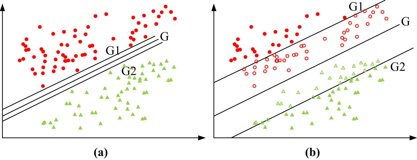
Effect of the penalty factor on the SVM. (a) Higher penalty factor, and (b) small penalty factor.
In Figure 2, when
3.2 SSA
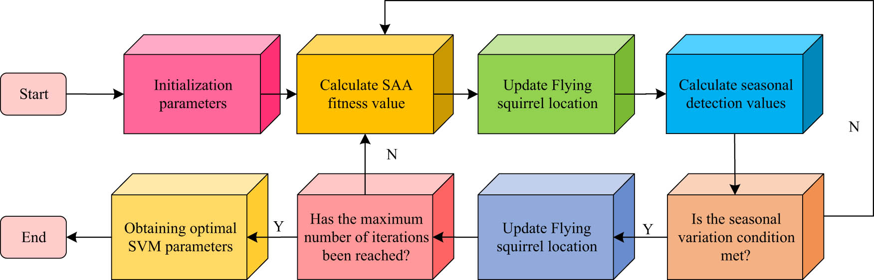
The SSA is a novel and powerful global swarm intelligence optimization algorithm. Penalty conditions and seasonal detection conditions are based on the algorithm’s inspiration, which is the natural foraging behavior of flying squirrels on various trees in the forest [23]. The workflow of the algorithm is shown in Figure 3.

Flow chart of the SSA work.
As shown in Figure 3, during initialization, the number of flying squirrels is set to
In the above equation, the position of each flying squirrel is randomized, and the squirrels can change their position at will to find food for the purpose of searching for the optimal solution. Using a uniform distribution to initialize the position of each flying squirrel, the initialization equation is shown in the following equation:
In the above equation,
In the above equation, the food sources are classified as superior, medium, and average, and the three food sources correspond to the optimal, sub-optimal, and feasible solutions, respectively. The results of the adaptations calculated by equation (8) are ranked in ascending order, with the flying squirrels with the smallest adaptations being located on the superior food source. The medium flying squirrels were located on the medium food source and had a tendency to fly toward the superior food source. The top-tier flying squirrels were found at the median food source. Moreover, flying squirrels with their satiety needs met gravitated toward the top-tier food source, while flying squirrels with unmet food needs veered toward the intermediate food source. All flying squirrels also adjust their flight direction to the food source according to the probability of predator presence. This process of repositioning is called location updating, and there are three main types of location updating. The first is when the flying squirrels fly from a medium food source to a high food source, and the equation for this is shown in the following equation:
In the above equation, the flying squirrel’s position on a medium food source is represented by FSat, its position on a superior food source by
In the above equation, the flying squirrel’s location on a general food supply is represented by
In the above equation,
In the above equation,
In the above equation,
4 Construction of a course evaluation model based on an improved algorithm
4.1 SSA-SVM
The SSA can be used to perform optimization of the SVM due to its good convergence and the fact that it is not easily trapped in a local optimum solution. The classification accuracy and calculation speed of the SVM algorithm can be enhanced by achieving the optimal value. Figure 4 depicts the workflow of the enhanced SVM algorithm using SSA.
Flow chart of the SSA optimized SVM algorithm.
In Figure 4, the flying squirrel’s position is initialized using the penalty factor as the optimization objective, and it is determined whether to update its position based on the calculated SSA adaptation value. The seasonal detection value is then calculated to avoid the situation of a local optimum solution. If the seasonal detection values do not satisfy the seasonal change conditions, the SSA adaptation values must be recalculated. Once the seasonal detection value has been satisfied, the location of the flying squirrel is updated once more. At this juncture, it is determined that the maximum number of iterations has been attained. In order to obtain the optimal response for the SVM parameters, it is necessary to sustain the method’s iterations until the requisite number of iterations has been reached, or conversely, until the maximum number of iterations has been attained.
4.2 Construction of quality evaluation index system for civil engineering budget course
In the course quality evaluation model, the quality evaluation index system of the civil engineering budgeting course needs to be constructed before the overall quality of the course can be evaluated. In view of this, the study has constructed a curriculum evaluation system for the civil engineering budgeting course, as shown in Table 2, by reviewing relevant data.
Curriculum evaluation system for civil engineering budget course
| Evaluation index system | Primary indicators | Secondary indicators | Indicator number |
|---|---|---|---|
| Curriculum evaluation indicators for civil engineering budget course | Teacher’s teaching skills and attitude | Language expression | Z1 |
| Pre class preparation | Z2 | ||
| Value orientation | Z3 | ||
| Teacher’s teaching method | Highlighting key and difficult points | Z4 | |
| Inspiring | Z5 | ||
| Detailed explanation | Z6 | ||
| Content | Complete | Z7 | |
| Frontiers | Z8 | ||
| Example demonstration | Z9 | ||
| Course | Novelty | Z10 | |
| Representativeness | Z11 | ||
| practicability | Z12 | ||
| Course updates | Z13 | ||
| Student learning behavior | Exchange and discussion | Z14 | |
| Review | Z15 | ||
| Sharing communication | Z16 | ||
| Self-evaluation | Z17 | ||
| Student learning effectiveness | Practical operation | Z18 | |
| Proficient mastery | Z19 | ||
| Deep learning | Z20 |
The assessment index system for the civil engineering budgeting course developed by the study, as indicated in Table 1, consists of a total of 6 primary indicators and 20 supplementary indicators. The six level 1 indicators are teacher teaching skills and attitudes, teacher teaching style, course content, course design, student learning behavior, and student learning outcomes. Once the indicators of the evaluation system of the course have been established, the study can employ the fusion algorithm to evaluate each secondary indicator of the teaching evaluation system, thereby identifying any issues in the civil engineering budgeting course. Subsequently, in order to enhance the overall quality of the civil engineering budgeting course and, consequently, the professional competence of civil engineering students, the evaluation system must be reinforced in order to address the shortcomings inherent in the evaluation system.
4.3 Evaluation model of improved budget course based on SSA-SVM
Civil engineering budgeting is the study of investment decisions for civil engineering projects. The discipline focuses on the budgeting and control of project costs based on the actual requirements of engineering design, materials and equipment, personnel and management [24,25]. In addition, the course’s also examines investment decisions for civil engineering projects, determining the cost of the project and developing the corresponding budget proposal. Civil engineering budgeting is a fundamental course that must be mastered by civil engineering and construction students. Through the analysis and calculation of these contents, the course assists students in mastering the fundamental knowledge and skills of civil engineering budgeting. The course focuses on the construction cost, project revenue, and profit of civil engineering projects. The quality of teaching in the civil engineering budgeting course is critical for civil engineering students. It enables them to select suitable financing methods and enhance the efficiency and effectiveness of construction projects through the estimation and financial analysis of the civil engineering budget. The study incorporates the SSA-SVM algorithm into the evaluation model of the civil engineering budgeting course in order to more accurately assess the teaching effectiveness of the current course. The teaching quality evaluation model that the study proposes is displayed in Figure 5.

Classroom quality evaluation model flow based on the SSA-SVM algorithm.
In Figure 5, the first stage of the evaluation model is to collect information about the civil engineering budgeting course and then construct an evaluation index system for the course. In the second step, the evaluation indicators from the teaching quality evaluation sample are collected and pre-processed before being fed into the SVM classification model. At the same time, the SSA is used to optimize the SVM classification model until the SVM model reaches the optimal parameters. The optimized SVM model is then used to evaluate the evaluation indicators in the test sample to obtain the evaluation results of the test sample. To determine the strengths and weaknesses of the course and to come up with effective solutions to improve the civil engineering budgeting course as a whole, the evaluation model is used to evaluate the indicators of the course. The SSA-SVM algorithm has potential value in evaluating civil engineering budget courses. However, its practical application comes with several costs. Implementing an evaluation model based on the SSA-SVM algorithm involves five potential costs. First, the algorithm needs extensive data processing and model training, which requires significant computer resources. This may require high-performance computers or multi-core processors, especially when working with large datasets. There are costs associated with purchasing and maintaining these hardware devices. Data collection is necessary prior to applying the SSA-SVM algorithm for the civil engineering budget course. Relevant data from various sources must be collected, which can involve human and time costs. Additionally, data cleaning and pre-processing are critical tasks that require time and manpower to process missing values, outliers, and noisy data to guarantee data quality and availability. Implementing SSA-SVM algorithms and applying them to evaluation models may necessitate specialized programming skills and machine learning knowledge. The developers need to spend time customizing, debugging, and fine-tuning algorithms to guarantee optimal performance and accuracy. The expense of model validation and testing constitutes the fourth point. A significant number of experiments and tests are necessary to confirm the effectiveness and performance of the SSA-SVM algorithm. Techniques such as cross-validation, hyperparameter tuning, and others help optimize the model. Verification and testing entail costs in terms of computational resources and time. The final consideration to take into account is the expenses associated with training and learning. Since the SSA-SVM algorithm comprises intricate mathematical and machine learning concepts, it may be necessary to incur additional expenses to guarantee that the team possesses adequate expertise to utilize the algorithm effectively. To conclude, when assessing the utilization of the SSA-SVM algorithm, it is crucial to fully assess these costs and establish a reasonable implementation strategy in compliance with the project’s budget and resources.
5 Experimental validation and empirical analysis
To verify the effectiveness of the improved SSA-SVM algorithm proposed in the study, its performance was compared and analyzed using four indicators: accuracy, precision, recall, and F1 value. Comparing the algorithm with the Back Propagation (BP) algorithm, genetic algorithm SVM (GA-SVM), and traditional SVM algorithm. The experimental environment was Matlab simulation software, and the training set and testing were UCI (University of California) datasets. The URL (Uniform resource location) of the UCI dataset is https://archive.ics.uci.edu/ml/datasets.php. The research pertains to the use of machine learning algorithms, predominantly the SSA-SVM algorithm, for enhancing and optimizing the assessment efficacy of civil engineering budget courses. The verification of algorithmic effectiveness necessitates the comparison and analysis of their performance across different algorithms. Hence, it is crucial to select appropriate evaluation indicators and datasets. The UCI dataset has been chosen based on its rationality. The UCI dataset is a public dataset provided by the University of California. It is extensively used by researchers and developers to assess and validate the proficiency of machine learning algorithms. The UCI dataset is highly regarded in the machine learning domain, enhancing the credibility of the research. The second reason is that the UCI dataset has an extensive range of datasets covering different areas and issues. This allows for the selection of appropriate datasets for the study’s topic, which can simulate real-world scenarios and allow for testing of algorithm performance. Additionally, UCI datasets commonly have annotated data available for training and testing. To align with the study’s theme, the relevant dataset “Civil Engineering Budget” was chosen. The dataset includes a significant number of budget cases of civil engineering, each marked with several characteristics and corresponding budget outcomes. This provides comprehensive information perfect for training and testing algorithms. Additionally, there are thousands of samples in the dataset, making it ideal for algorithm performance evaluation. The dataset comprises diverse elements that relate to civil engineering budgets, including project type, location, materials, and design complexity, amongst others. The features are represented as numerical data for straightforward processing by algorithms. However, before utilizing the data from this dataset, pre-processing is necessary. Initially, data cleaning is performed to remove samples with missing or incorrect values to ensure data accuracy and completeness. Feature normalization is then applied to scale all feature values between [0,1]. This eliminates dimensional disparities between different features. Afterward, the dataset will be split into a training and test set to both train the algorithm and evaluate its performance. The training set will comprise 70%–80% of the data, while the test set will account for the remaining 20% to 30%. The feature engineering component of this study principally includes conducting correlation analyses. Calculating the correlation between features, highly correlated features are deleted to reduce feature redundancy and improve algorithm efficiency. Next, the feature selection algorithm selects the most relevant features to optimize the model’s performance. These pre-processing and feature engineering steps enhance the utilization of UCI datasets and verify the effectiveness of the SSA-SVM algorithm in evaluating civil engineering budget courses.
5.1 Comparative performance analysis of the improved SSA-SVM algorithm
5.1.1 Determine the optimal parameters of the SVM model
The performance and accuracy of SVM is significantly impacted by its parameter settings. Varying parameter combinations can yield vastly different model performance. Therefore, prior to model training, parameter optimization is essential to achieve optimal SVM performance and success in future tasks. To ensure the accuracy of the SVM, certain parameters like the penalty coefficient C and kernel function parameters must have a reasonable range of values established. To provide an example, the study considered a penalty coefficient range of [0.1, 1000]. Utilizing the SSA, internal data structures can be analyzed to find the optimal parameter combination to enhance parameter exploration efficiency and attain the ideal combination for SVM. To ensure the accuracy of the parameter combination, the three-way cross-validation method is adopted. The dataset is divided into three parts – two for training and one for validation. This division is done three times, with a different part selected as the verification set each time. This generates a more precise evaluation of the performance of the model on various data subsets. Along with programming experiments, the accuracy of the training set is established to guarantee that the selected parameters are not only reasonable in theory but also applicable in practice. The penalty coefficient C is a crucial parameter in SVM, governing the penalty for misclassification. A higher value of C commands a greater penalty for erroneous or false samples, resulting in minimal classification errors. Conversely, a lower value of C implies that the classifier may not be as concerned about misclassification. In this study, the range of values for C is set to [0.1, 1000]. To allow the algorithm to find the optimal value within a wide range that takes into account the possible variations in C from small to large. A C value that is too large may lead to overfitting, while a too small value may result in underfitting. Additionally, the kernel function is a crucial parameter in SVM that determines the representation of the data in a high-dimensional space. The chosen γ value for this dataset is 0.075, based on accumulated experiments and experience as the kernel function for this study. The SSA’s exploration and development capacity is dependent on its cross-probability. The study’s crossover probability value is 0.7, indicating a 70% chance of performing a crossover operation during each iteration. This probability assists the algorithm in preserving strong exploration ability and avoiding local optimums. The selected value is informed by the experiment’s observations and is determined to balance exploration and exploitation, thereby enhancing the algorithm’s efficiency in obtaining optimal solutions. The variation probability improves the local search capabilities of the SSA and prevents falling into local optima. The mutation probability value for this study is 0.1, indicating a 10% probability of mutation operation in each iteration. This low probability maintains the current solution most of the time, but small random perturbations are made in some cases to prevent the algorithm from falling into a local optimal solution. The selection of this parameter is informed by the outcomes of numerous experiments, indicating that a mutation probability of 0.1 effectively prevents premature convergence of the algorithm to suboptimal solutions while maintaining search efficiency. The results of the genetic algorithm fitness change curve during testing are shown in Figure 6.

Fitness curve of the genetic algorithm during testing.
During the testing of SSA-SVM, the fitness curve depicts the changes in the SVM’s performance as the algorithm advances. The fitness mainly depends on accuracy, which is computed by dividing the number of correctly classified samples by the total number of samples. The accuracy of the SVM model under different specific parameters is illustrated by the fitness. Figure 6 shows that as the number of population evolution generations increases, both the average fitness curve and the best fitness curve show an overall upward trend, and the final fitness of the best fitness curve is stable at 95.6. In addition, it can also be concluded from Figure 6 that the optimal penalty coefficient obtained through training is 31.216, at which point the accuracy of the model classification reaches 95.6%. To build the model using the SSA-SVM algorithm, the determined optimal parameters were added to the initial SVM model.
5.1.2 Verifying the effectiveness of SSA-SVM prediction models using public datasets
After obtaining the SSA-SVM algorithm model, use the training set to train the SSA-SVM model and obtain the SSA-SVM prediction model. Figure 7 displays the outcomes of the SSA-SVM algorithm on both the training and test sets.

Square correlation coefficient and mean square error test results of the training set and test set. (a) Prediction results of training samples and (b) prediction results of test samples.
The regression model’s performance is commonly evaluated using the square correlation coefficient and the mean square error. The square correlation coefficient, also referred to as the coefficient of determination, determines how well the model comprehends the data. The squared correlation coefficient is computed by subtracting the residual sum of squares from one and dividing the result by the total sum of squares quotient. The coefficient’s range is between 0 and 1. A value closer to 1 indicates a stronger correlation between the predicted and actual model values and a better fit for the model. The mean square error measures the average squared discrepancy between the model’s predicted value and the actual value. The calculation method involves three steps. First, the squared difference between the predicted value and the actual value of each sample is calculated. Then, the sum of all the squared differences is divided by the number of samples, n, resulting in the mean squared error. A smaller mean squared error indicates a higher level of accuracy in the model’s predictions. From Figure 7(a), the value of the squared correlation coefficient of the SSA-SVM algorithm in the training set is 0.9189 and the value of the mean squared error is 0.00628, both of which indicate that the SSA-SVM algorithm has a high accuracy in the training set. As the value of the squared correlation coefficient is greater than 0.85, this result also indicates that the SSA-SVM algorithm has a high generalization ability in the training set. According to Figure 7(b), the mean squared error and squared correlation coefficient of the test sample for the SSA-SVM algorithm were 0.8709 and 0.01309, respectively. According to the above results, the SSA-SVM algorithm proposed in this article performs better on the training and test sets.
5.1.3 Performance comparison and analysis of SSA-SVM prediction models
The study used comparison experiments with the Genetic Algorithm-Back Propagation (GA-BP), GA-SVM, and Back Propagation-Support Vector Machine (BP-SVM) algorithms on Matlab simulation software and evaluated the performance with accuracy, precision, recall, and F1 value as the comparison index in order to confirm the efficacy of the SSA-SVM technique suggested in the study for analysis [26,27]. The reasons for selecting these comparison algorithms are as follows: The BP algorithm is a frequently used an artificial neural network algorithm that is widely used in classifying and solving regression issues. It has a relatively simple principle and implementation and shows improvement in many problems. This article compares the SSA-SVM algorithm with the BP algorithm to demonstrate the superiority and improvement of the former over the latter in terms of traditional neural network algorithms. SVM is a well-established machine learning algorithm with exceptional performance in solving both classification and regression problems. It serves as the foundation for the SSA-SVM algorithm, which aims to demonstrate the degree of improvement attained by introducing SSA fusion. The GA-SVM algorithm, a hybrid optimization algorithm that combines a genetic algorithm with SVM, is capable of performing a powerful global search and can effectively optimize SVM parameters. The efficacy and superiority of the SSA in SVM parameter optimization can be verified when compared to the GA-SVM algorithm. Figure 8 displays the accuracy outcomes for the four methods in the same training set.

Comparison of prediction accuracy of four algorithms in the same dataset.
In Figure 8, among the four algorithms, the SSA-SVM algorithm has the highest overall accuracy, and its highest accuracy is 0.927, which is higher than the GA-SVM algorithm’s 0.803, the BP-SVM algorithm’s 0.679, and the GA-BP algorithm’s 0.646. According to the above results, the SSA-SVM method performs better in terms of accuracy than the three algorithms studied.
5.1.4 Comparison of Receiver Operating Characteristic (ROC) and Precision-Recall (PR) curves of SSA-SVM prediction model
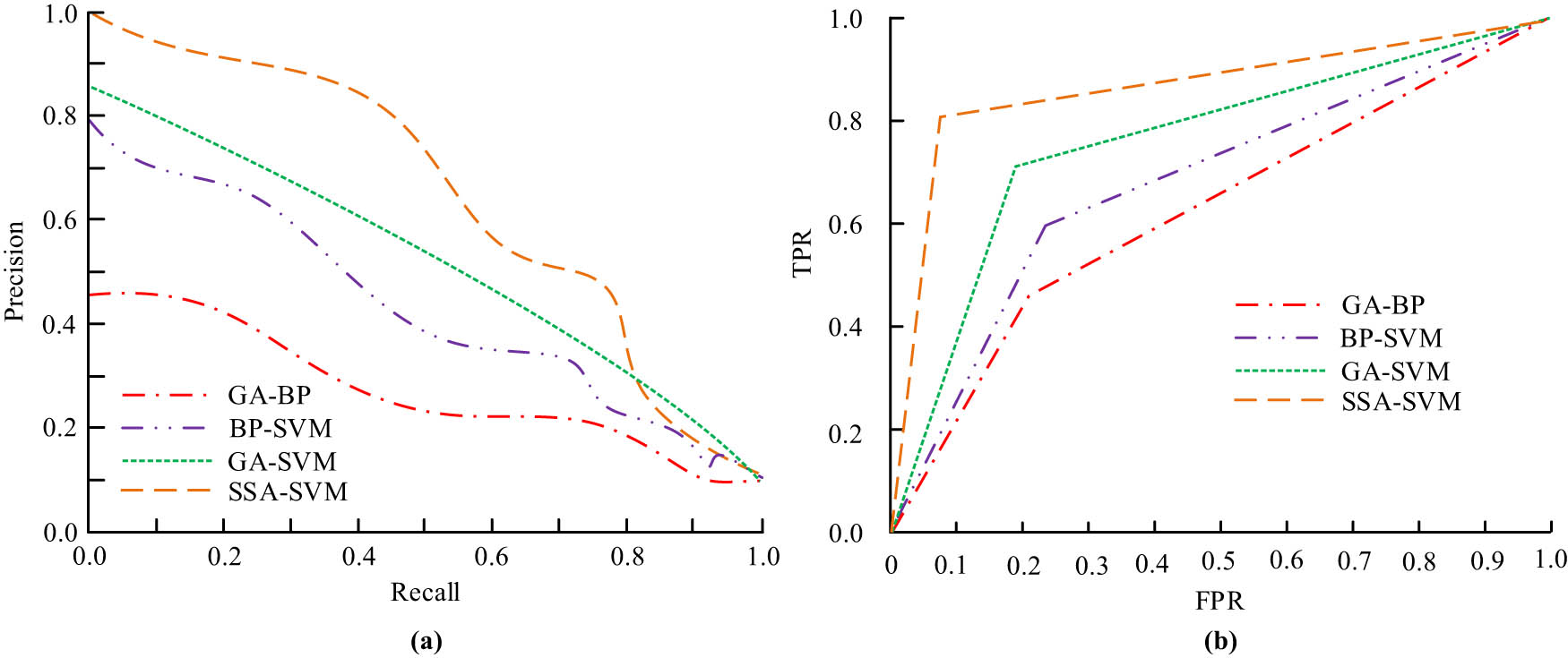
Further performance comparison and analysis of the algorithms proposed in the study, the results of the ROC curves and precision–recall (PR) curves for the four algorithms are shown in Figure 9.
ROC and PR curves of four algorithms. (a) PR curve and (b) ROC curve.
Figure 9(a) shows that the SSA-SVM approach has a significantly higher area under the PR curve than the other algorithms, with an area under the PR curve line of 0.78. In Figure 9(b), the area under the ROC curve of the SSA-SVM algorithm is also significantly higher than the other algorithms, with an area under the ROC curve line of 0.84. The above results show that, in terms of PR curve and ROC curve dimensions, the performance of the SSA-SVM algorithm is superior to that of the GA-SVM, BP-SVM, and GA-BP algorithms.
5.1.5 Comparison of percentage error and mean absolute error of SSA-SVM prediction model
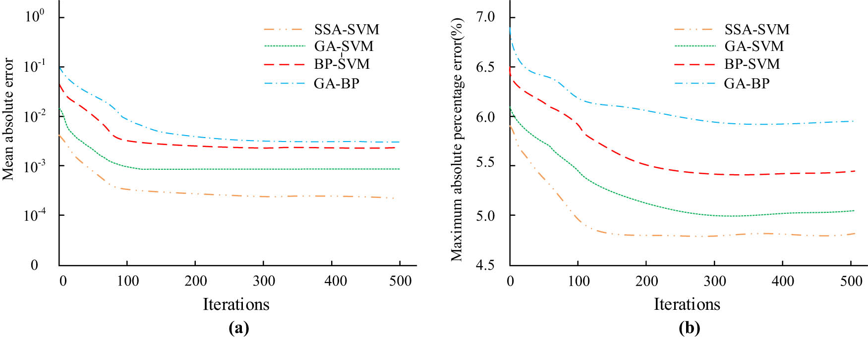
The results of the mean absolute error and the maximum absolute percentage error of the four algorithms with the number of iterations are shown in Figure 10.
Compare the average absolute error and maximum absolute percentage error of four algorithms. (a) Mea absolute error, and (b) maximum absolute percentage error.
In accordance with Figure 10(a), the SSA-SVM approach has the lowest average absolute error among the four algorithms at 0.00147, which is lower than that of the GA-SVM algorithm at 0.00618, the BP-SVM algorithm at 0.00824 and the BP algorithm at 0.00889. From Figure 10(b), the maximum absolute percentage error is the lowest among the four algorithms at 4.8%, which is lower than the 5.1% of the GA-SVM algorithm, 5.4% of the BP-SVM algorithm, and 5.9% of the GA-BP algorithm. These results showed that the SSA-SVM algorithm outperformed the comparison algorithms in terms of the error dimension. Combining the results of the above dimensions, the prediction performance of the SSA-SVM algorithm proposed in the study is much better than that of other similar algorithms. Therefore, the study applies it to the evaluation model of the civil engineering budgeting course, which is expected to improve the accuracy of the evaluation model and provide data support for the improvement of the civil engineering budgeting course.
5.1.6 Comparison of accuracy rate and recall rate of SSA-SVM prediction model
Then, the accuracy rate and recall rate of the four algorithms in the UCI dataset are compared, and the comparison curve is shown in Figure 11.

Comparison results of accuracy and recall rate of four algorithms in UCI dataset. (a) Precision comparison results, and (b) comparison of recall rates.
Figure 11(a) shows that the accuracy curves of the four SSA-SVM algorithms are higher than those of the other three comparison algorithms. The average accuracy is 95.6%, which exceeds that of the GA-SVM algorithm (90.3%), BP-SVM algorithm (79.9%), and GA-BP algorithm (73.5%). As shown in Figure 11(b), the recall rate curves of the SSA-SVM algorithm are higher than those of the other three comparison algorithms. The average recall rate of the SSA-SVM algorithm is 92.2%, which surpasses the GA-SVM algorithm (87.5%), the BP-SVM algorithm (84.3%), and the GA-BP algorithm (81.9%). These findings indicate that the SSA-SVM algorithm outperforms the three comparison algorithms in terms of accuracy and recall rate.
5.1.7 Analysis of F1 comparison results of SSA-SVM prediction model
The F1 value results of the four algorithms are shown in Figure 12.

Comparison results of F1 values of the four algorithms.
Figure 12 shows that the F1 value curves of SSA-SVM are higher than those of the other three comparison algorithms. In addition, its highest recall rate is 0.94, compared to the GA-SVM algorithm (0.92), the BP-SVM algorithm (0.87), and the GA-BP algorithm (0.65). Based on the above dimensions, the proposed SSA-SVM algorithm has better prediction performance than other similar algorithms. Therefore, the study applied it to the evaluation model of the civil engineering budget estimate course, hoping to improve the accuracy of the evaluation model and provide data support for the improvement of the civil engineering budget estimate course.
5.2 Empirical analysis of the evaluation model
The study examined five classes of civil engineering students at a university as research subjects. These classes were selected due to their representation of the previous year’s course performance and inclusion of students from various grades, enabling a thorough evaluation of the model’s aptness for students at different levels. To ensure the credibility and validity of the data, the classes with incomplete or clearly anomalous data are excluded. The process for collecting data is as follows. Initially, a set of evaluation indicators were determined based on the characteristics of the civil engineering budget course. After determining the evaluation indicators, the University’s academic Affairs Office provided the specific values of each indicator for each student in the five classes. The original data was then collected, followed by data cleaning, pre-processing, and normalization, including processing missing values and outliers. According to the mentioned feature engineering method, the correlation analysis and feature selection of the selected evaluation indicators are carried out to further optimize the performance of the model. By comparing the actual results of various indicators of the budget course with the evaluation results of traditional budget courses, the evaluation performance of the improved budget course cost-effectiveness model proposed by Padula et al. is analyzed [28].
5.2.1 Analysis of the application effect of the improved budget course evaluation model
Five classes of students at a university with a civil engineering major served as research subjects to investigate the practical applicability of the civil engineering budgeting course evaluation model that utilized the SSA-SVM algorithm. Both the SSA-SVM algorithm-based evaluation model and the conventional course evaluation model were applied to evaluate the civil engineering budgeting course in these five classes. The precise evaluation findings are displayed in Table 3.
Evaluation results of various evaluation indicators for civil engineering budget course courses
| Primary indicators | Secondary indicators | Index number | Actual results | The evaluation model results in this article | Traditional evaluation model results |
|---|---|---|---|---|---|
| Primary indicators | Language expression | Z1 | 0.81 | 0.77 | 0.75 |
| Pre-class preparation | Z2 | 0.79 | 0.76 | 0.71 | |
| Value orientation | Z3 | 0.82 | 0.80 | 0.75 | |
| Teacher’s teaching skills and attitude | Highlighting key and difficult points | Z4 | 0.77 | 0.75 | 0.80 |
| Inspiring | Z5 | 0.85 | 0.84 | 0.89 | |
| Detailed explanation | Z6 | 0.86 | 0.87 | 0.92 | |
| Teacher’s teaching method | Complete | Z7 | 0.91 | 0.89 | 0.85 |
| Frontiers | Z8 | 0.92 | 0.91 | 0.86 | |
| Example demonstration | Z9 | 0.91 | 0.89 | 0.81 | |
| Content | Novelty | Z10 | 0.88 | 0.91 | 0.85 |
| Representativeness | Z11 | 0.85 | 0.85 | 0.78 | |
| Practicability | Z12 | 0.93 | 0.91 | 0.83 | |
| Course updates | Z13 | 0.86 | 0.91 | 0.81 | |
| Course | Exchange and discussion | Z14 | 0.88 | 0.89 | 0.81 |
| Review | Z15 | 0.90 | 0.90 | 0.82 | |
| Sharing communication | Z16 | 0.91 | 0.91 | 0.79 | |
| Self-evaluation | Z17 | 0.86 | 0.85 | 0.75 | |
| Student learning behavior | Practical operation | Z18 | 0.93 | 0.92 | 0.86 |
| Proficient mastery | Z19 | 0.86 | 0.85 | 0.80 | |
| Deep learning | Z20 | 0.84 | 0.89 | 0.82 |
The evaluation results for each indicator of the civil engineering budgeting course are shown in Table 3 using two different evaluation models. The standard evaluation methodology for the Civil Engineering Budgeting course is often less accurate than the SSA-SVM course evaluation model proposed in the study, as shown in Table 3. Based on these results, the SSA-SVM course evaluation model has a better evaluation performance. SSA-SVM is a superior model.
5.2.2 Improving the evaluation model of budgeting curriculum and its impact on students
Student learning efficiency and student satisfaction were used as evaluation indicators before and after the course was improved by the evaluation model in the 3-week experiment in order to compare the effects of the proposed evaluation model on the course. The results of student learning efficiency and student satisfaction scores over 3 weeks are shown in Figure 13.

Student learning satisfaction and exam score results within 3 months. (a) Student satisfaction ad (b) student learning efficiency.
Figure 13 shows the specific changes in student satisfaction and exam scores within 3 months of the improvement of the civil engineering budgeting course using the GA-BP course evaluation model proposed in the study. In Figure 13, student satisfaction and student examination scores increased significantly within 3 months of the improvement of the Civil Engineering Budgeting course using the proposed course evaluation model. The student satisfaction and academic performance scores are found to be 92 and 94, respectively, representing a significant improvement over the previous scores. From the above results, it is clear that the SSA-SVM course evaluation model proposed in the study has made a great contribution to the civil engineering budgeting course. As a result, the model can be used to improve the civil engineering budgeting course, which will improve the teaching effectiveness of the course and the overall aptitude of the students. The features employed in the assessment model are widely available and can be applied to other courses and disciplines. The SSA-SVM algorithm primarily assesses course quality by estimating features in the evaluation model, facilitating its use in evaluating other courses.
6 Conclusion
The SSA-SVM algorithm, which was created by combining the SSA and SVM algorithms, was then incorporated into the civil engineering budgeting course evaluation model in order to increase the accuracy of the model. This study employs the SSA-SVM algorithm to assess each evaluation index of the evaluation model for the civil engineering budget estimation course to identify strengths and weaknesses and enhance it. The experimental results indicated that the proposed algorithm was effective in improving the accuracy of the model, and its accuracy reached 0.927, which surpassed GA-SVM, BP-SVM, and GA-BP algorithms. In terms of performance comparison, the SSA-SVM algorithm obtained an average absolute error of 0.00147, which was lower than that of the GA-SVM algorithm of 0.06, which further proves the superiority of the SSA-SVM algorithm. Based on empirical analysis, it was found that after the course evaluation model of civil engineering probabilistic budgeting proposed in this study was adopted for course improvement, the students’ satisfaction scores and examination scores were significantly improved, from 70 to 92 and from 75 to 94, respectively. The findings revealed that the evaluation model had practical guidance significance and application value for curriculum improvement. Additionally, the model’s performance was found to be closely related to the quality of the input data. High-quality data can enhance the model’s predictive accuracy and stability, while outliers, noise, or erroneous data may negatively impact its performance. When using the SSA-SVM algorithm, it is crucial to fully pre-process the data to enhance the model’s performance. The main conclusions drawn from the study include the following efficacy of the SSA-SVM algorithm in evaluating civil engineering budget courses, while also guiding future research in this field. The accuracy of the SSA-SVM algorithm was found to be 0.927, higher than that of the GA-SVM algorithm at 0.803, the BP-SVM algorithm at 0.679, and the GA-BP algorithm at 0.646. The performance of the SSA-SVM algorithm was compared with the GA-SVM, BP-SVM, and GA-BP algorithms. In addition, the mean absolute error of the optimization algorithm was lower than that of the GA-SVM algorithm, which was 0.06, at 0.00147 compared to 0.006. The results of the empirical analysis of the course evaluation model of the civil engineering probabilistic budgeting method proposed in the study then showed that after the course improvement using the course evaluation model, the students’ satisfaction score increased from 70 to 92; the students’ examination score increased from 75 to 94. After comparing the evaluation model with the experimental results, it was determined that the civil engineering budget estimate course evaluation model performed better than the comparison model. The findings indicate that the proposed optimization algorithm and evaluation model outperformed the alternatives. The superior performance of the evaluation model proposed in this study primarily results from the effective optimization achieved by integrating the SSA and SVM algorithms. The SSA adjusts the parameters of the SVM algorithm, resulting in the improved performance of the SSA-SVM algorithm, consequently leading to an accurate classification. This optimization approach enhances the precision and robustness of the model. The research above illustrates a successful improvement of the precision of the evaluation model for civil engineering budget courses through the integration of the SSA and SVM algorithms. However, there exist some limitations in the study. For instance, although the SSA-SVM algorithm demonstrated good performance in this study, its effectiveness cannot be guaranteed in all scenarios and datasets. The algorithm’s general applicability needs testing under varying environments and datasets. Additionally, the SSA-SVM algorithm may encounter overfitting problems. Overfitting can lead to poor performance of the model on new data. In addition, the quality of the input data significantly affects the performance of the SSA-SVM evaluation model. If there are noise, outliers, or errors in the data, the model’s performance may suffer. Therefore, future studies utilizing the SSA-SVM algorithm should consider various factors, including model complexity, data volume, data quality, and parameter settings. Adopting appropriate strategies and methods is crucial to avoid overfitting and bias and to ensure accurate and stable evaluation results.
Corresponding meaning of the symbol
| Symbol | Explain |
|---|---|
|
|
Normal vector |
|
|
Bias |
|
|
Minimization confidence range |
|
|
Slack variables |
|
|
Penalty factor |
|
|
Position of the
|
|
|
Flying rat serial number |
|
|
Dimension of the flying squirrel |
|
|
Upper boundary of the flying squirrel guard position |
|
|
Lower boundary of the flying squirrel position |
|
|
The flying squirrel’s position on a medium food source |
|
|
The flying squirrel’s position on a superior food source |
|
|
The flying squirrel’s glide step |
|
|
The flying squirrel’s glide constant |
|
|
The number of iteration |
|
|
Likelihood of encountering a predator |
|
|
The flying squirrel’s location on a general food supply |
|
|
Seasonal constant |
|
|
Minimum value of the seasonal constant |
|
|
The Levy flight acquisition step approach |
-
Funding information: This work is supported by Cultivation Project for Innovative Scientific and Educational Groups ZCKC23011; Fuzhou University Zhicheng College Applied Undergraduate Course – Civil Engineering Construction ZJ2312.
-
Author contributions: All authors contributed to the study conception, design, material preparation, data collection, and analysis. All authors read and approved the final manuscript.
-
Conflict of interest: Authors state no conflict of interest.
References
[1] S. Try, K. Panuwatwanich, G. Tanapornraweekit and M. Kaewmoracharoen, Virtual reality application to aid civil engineering laboratory course: A multicriteria comparative study, Comput. Appl. Eng. Educ. 29, (2021), no. 6, 1771–1792, DOI: https://doi.org/10.1002/cae.22422.10.1002/cae.22422Suche in Google Scholar
[2] B. H. W. Guo, M. Milke and R. Jin, Civil engineering students’ perceptions of emergency remote teaching: a case study in New Zealand, Eur. J. Eng. Educ. 47 (2022), no. 4 679–696, DOI: https://doi.org/10.1080/03043797.2022.2031896.10.1080/03043797.2022.2031896Suche in Google Scholar
[3] S. Choudhuri, S. Adeniye and A. Sen, Distribution alignment using complement entropy objective and adaptive consensus-based label refinement for partial domain adaptation, Artif. Intell. Appl. 1 (2023), no. 1, 43–51, DOI: https://doi.org/10.47852/bonviewaia2202524.10.47852/bonviewAIA2202524Suche in Google Scholar
[4] D. Rostini, R. Z. A. Syam and W. Achmad, The significance of principal management on teacher performance and quality of learning, Al-Ishlah: Jurnal Pendidikan 14 (2022), no. 2, 2513–2520, DOI: https://doi.org/10.35445/alishlah.v14i2.1721.10.35445/alishlah.v14i2.1721Suche in Google Scholar
[5] Y. Wu, X. Sun, B. Dai, P. Yang and Z. Wang, A transformer fault diagnosis method based on hybrid improved grey wolf optimization and least squares-support vector machine, IET Gener. Transm. Dis. 16 (2022), no. 10, 1950–1963, DOI: https://doi.org/10.1049/gtd2.12405.10.1049/gtd2.12405Suche in Google Scholar
[6] X. B. Liu, Y. L. Guan and Q. Xu, Support vector machine-based blind equalization for high-order QAM with short data lengt, IEEE Signal Process. Lett. 28 (2021), no. 12, 259–263, DOI: https://doi.org/10.1109/LSP.2021.3050928.10.1109/LSP.2021.3050928Suche in Google Scholar
[7] X. M. Long, Y. J. Chen and J. Zhou, Development of AR experiment on electric-thermal effect by open framework with simulation-based asset and user-defined input, Artif. Intell. Appl. 1 (2023), no. 1, 52–57, DOI: https://doi.org/10.47852/bonviewaia2202359.10.47852/bonviewAIA2202359Suche in Google Scholar
[8] A. Khare and S. Agrawal, Scheduling hybrid flowshop with sequence-dependent setup times and due windows to minimize total weighted earliness and tardiness, Comput. Ind. Eng. 135 (2019), no. 6, 780–792, DOI: https://doi.org/10.1016/j.cie.2019.06.057.Suche in Google Scholar
[9] Q. W. Dong, S. M. Wang, F. J. Han and R. D. Zhang, Innovative research and practice of teachers’ teaching quality evaluation under the guidance of ‘innovation and entrepreneurship’, Procedia Comput. Sci. 154 (2019), no. 5, 770–776, DOI: https://doi.org/10.1016/j.procs.2019.06.123.10.1016/j.procs.2019.06.123Suche in Google Scholar
[10] J. Yang, L. Shen, X. Jin, L. Hou, S. Shang and Y. Zhang, Evaluating the quality of simulation teaching in Fundamental Nursing Curriculum: AHP-Fuzzy comprehensive evaluation, Nurse Educ. Today 77 (2019), no. 77, 77–82. DOI: https://doi.org/10.1016/j.nedt.2019.03.012.10.1016/j.nedt.2019.03.012Suche in Google Scholar PubMed
[11] A. Ls, Y. B. Jing, B. Xj, J. Xiao, H. Luo, S. Shao and Z. Yan, Based on delphi method and analytic hierarchy process to construct the evaluation index system of nursing simulation teaching quality, Nurse Educ. Today 79 (2019), no. 5, 67–73, DOI: https://doi.org/10.1016/j.nedt.2018.09.021.10.1016/j.nedt.2018.09.021Suche in Google Scholar PubMed
[12] L. Bao and P. Yu, Evaluation method of online and offline hybrid teaching quality of physical education based on mobile edge computing, Mob. Netw. Appl. 6 (2021), no. 1, 1–11, DOI: https://doi.org/10.1007/s11036-021-01774-w.10.1007/s11036-021-01774-wSuche in Google Scholar
[13] R. Harrison, L. Meyer, P. Rawstorne, H. Razee, U. Chitkara, S. Mears and C. Balasooriya, Evaluating and enhancing quality in higher education teaching practice: A meta-review, Stud. High. Educ. 47 (2022), no. 1, 80–96, DOI: https://doi.org/10.1080/03075079.2020.1730315.10.1080/03075079.2020.1730315Suche in Google Scholar
[14] B. L. Lee and J. Johnes, Using network DEA to inform policy: The case of the teaching quality of higher education in England, High. Educ. Q. 76 (2022), no. 2, 399–421. DOI: https://doi.org/10.1111/hequ.12307.10.1111/hequ.12307Suche in Google Scholar
[15] B. Hca, B. Jd, Y. B. Rui, C. Vvp and D. Jwgg, Prediction of penetration rate by coupled simulated annealing-least square support vector machine (CSA_LSSVM) learning in a hydrocarbon formation based on drilling parameters, Energy Rep. 7 (2021), no. 4, 3971–3978, DOI: https://doi.org/10.1016/j.egyr.2021.06.080.10.1016/j.egyr.2021.06.080Suche in Google Scholar
[16] J. Zhang, J. Sun and H. He, Clustering detection method of network intrusion feature based on support vector machine and LCA Block algorithm, Wirel. Pers. Commun. 3 (2021), no. 5, 1–15, DOI: https://doi.org/10.1007/s11277-021-08353-y.10.1007/s11277-021-08353-ySuche in Google Scholar
[17] J. Song, C. Yu and S. Li, Continuous prediction of onsite PGV for earthquake early warning based on least squares support vector machine (in Chinese), Chin. J. Geophys 64 (2021), no. 2, 555–568, DOI: https://doi.org/10.6038/cjg2021O0193.Suche in Google Scholar
[18] M. Basu, Squirrel search algorithm for multi-region combined heat and power economic dispatch incorporating renewable energy sources, Energy 182 (2019), no. 1, 296–305, DOI: https://doi.org/10.1016/j.energy.2019.06.087.10.1016/j.energy.2019.06.087Suche in Google Scholar
[19] A. Khare and S. Agrawal, Scheduling hybrid flowshop with sequence-dependent setup times and due windows to minimize total weighted earliness and tardiness, Comput. Ind. Eng. 135 (2019), no. 7, 780–792, DOI: https://doi.org/10.1016/j.cie.2019.06.057.10.1016/j.cie.2019.06.057Suche in Google Scholar
[20] H. Zhang, Z. Wang, J. Liu, J. Chai and C. Wei, Selection of targeted poverty alleviation policies from the perspective of land resources-environmental carrying capacity, J. Rural Stud. 93 (2022), no. 3, 318–325, DOI: https://doi.org/10.1016/j.jrurstud.2019.02.011.10.1016/j.jrurstud.2019.02.011Suche in Google Scholar
[21] P. S. Neethu, R. Suguna and P. S. Rajan, Performance evaluation of SVM-based hand gesture detection and recognition system using distance transform on different data sets for autonomous vehicle moving applications, Circuit World 48 (2022), no. 2, 204–214, DOI: https://doi.org/10.1108/CW-06-2020-0106.10.1108/CW-06-2020-0106Suche in Google Scholar
[22] L. Luthfiana, J. C. Young and A. Rusli, Implementasi algoritma support vector machine dan chi square untuk analisis sentimen user feedback aplikasi, Ultimatics 12 (2020), no. 2, 125–126, DOI: https://doi.org/10.31937/ti.v12i2.1828.10.31937/ti.v12i2.1828Suche in Google Scholar
[23] S. Lee and J. H. Kim, Improvement of the support vector machine-based monte carlo simulation for calculating failure probability, Trans. Korean Soc. Mech. Eng. A 44 (2020), no. 4, 269–279, DOI: https://doi.org/10.3795/KSME-A.2020.44.4.269.10.3795/KSME-A.2020.44.4.269Suche in Google Scholar
[24] A. Islam, F. Othman and N. Sakib, Prevention of shoulder-surfing attack using shifting condition with the digraph substitution rules, Artif. Intell. Appl. 1 (2023), no. 1, 58–68. DOI: https://doi.org/10.48550/arXiv.2305.06549.10.47852/bonviewAIA2202289Suche in Google Scholar
[25] G. Eappen, T. Shankar and R. Nilavalan, Advanced squirrel algorithm-trained neural network for efficient spectrum sensing in cognitive radio-based air traffic control application, IET Commun. 15 (2021), no. 10, 1326–1351. DOI: https://doi.org/10.1049/cmu2.12111.10.1049/cmu2.12111Suche in Google Scholar
[26] K. Triolascarya, R. R. Septiawan and I. Kurniawan, QSAR study of larvicidal phytocompounds as anti-aedes aegypti by using GA-SVM method, RESTI 6 (2022), no. 4, 632–638. DOI: https://doi.org/10.29207/resti.v6i4.4273.10.29207/resti.v6i4.4273Suche in Google Scholar
[27] A. Kurani, P. Doshi, A. Vakharia and M. Shah, A comprehensive comparative study of artificial neural network (ANN) and support vector machines (SVM) on stock forecasting, Ann. Data Sci. 10 (2023), no. 1, 183–208. DOI: https://doi.org/10.1007/s40745-021-00344-x.10.1007/s40745-021-00344-xSuche in Google Scholar
[28] W. V. Padula, J. S. Levin, J. Lee and G. F. Anderson, Cost-effectiveness of total state coverage for hepatitis C medications, Am. J. Manag. Care. 27 (2021), no. 5, 171–177, DOI: https://doi.org/10.37765/ajmc.2021.88640.10.37765/ajmc.2021.88640Suche in Google Scholar PubMed
© 2024 the author(s), published by De Gruyter
This work is licensed under the Creative Commons Attribution 4.0 International License.
Artikel in diesem Heft
- Regular Articles
- On the p-fractional Schrödinger-Kirchhoff equations with electromagnetic fields and the Hardy-Littlewood-Sobolev nonlinearity
- L-Fuzzy fixed point results in ℱ -metric spaces with applications
- Solutions of a coupled system of hybrid boundary value problems with Riesz-Caputo derivative
- Nonparametric methods of statistical inference for double-censored data with applications
- LADM procedure to find the analytical solutions of the nonlinear fractional dynamics of partial integro-differential equations
- Existence of projected solutions for quasi-variational hemivariational inequality
- Spectral collocation method for convection-diffusion equation
- New local fractional Hermite-Hadamard-type and Ostrowski-type inequalities with generalized Mittag-Leffler kernel for generalized h-preinvex functions
- On the asymptotics of eigenvalues for a Sturm-Liouville problem with symmetric single-well potential
- On exact rate of convergence of row sequences of multipoint Hermite-Padé approximants
- The essential norm of bounded diagonal infinite matrices acting on Banach sequence spaces
- Decay rate of the solutions to the Cauchy problem of the Lord Shulman thermoelastic Timoshenko model with distributed delay
- Enhancing the accuracy and efficiency of two uniformly convergent numerical solvers for singularly perturbed parabolic convection–diffusion–reaction problems with two small parameters
- An inertial shrinking projection self-adaptive algorithm for solving split variational inclusion problems and fixed point problems in Banach spaces
- An equation for complex fractional diffusion created by the Struve function with a T-symmetric univalent solution
- On the existence and Ulam-Hyers stability for implicit fractional differential equation via fractional integral-type boundary conditions
- Some properties of a class of holomorphic functions associated with tangent function
- The existence of multiple solutions for a class of upper critical Choquard equation in a bounded domain
- On the continuity in q of the family of the limit q-Durrmeyer operators
- Results on solutions of several systems of the product type complex partial differential difference equations
- On Berezin norm and Berezin number inequalities for sum of operators
- Geometric invariants properties of osculating curves under conformal transformation in Euclidean space ℝ3
- On a generalization of the Opial inequality
- A novel numerical approach to solutions of fractional Bagley-Torvik equation fitted with a fractional integral boundary condition
- Holomorphic curves into projective spaces with some special hypersurfaces
- On Periodic solutions for implicit nonlinear Caputo tempered fractional differential problems
- Approximation of complex q-Beta-Baskakov-Szász-Stancu operators in compact disk
- Existence and regularity of solutions for non-autonomous integrodifferential evolution equations involving nonlocal conditions
- Jordan left derivations in infinite matrix rings
- Nonlinear nonlocal elliptic problems in ℝ3: existence results and qualitative properties
- Invariant means and lacunary sequence spaces of order (α, β)
- Novel results for two families of multivalued dominated mappings satisfying generalized nonlinear contractive inequalities and applications
- Global in time well-posedness of a three-dimensional periodic regularized Boussinesq system
- Existence of solutions for nonlinear problems involving mixed fractional derivatives with p(x)-Laplacian operator
- Some applications and maximum principles for multi-term time-space fractional parabolic Monge-Ampère equation
- On three-dimensional q-Riordan arrays
- Some aspects of normal curve on smooth surface under isometry
- Mittag-Leffler-Hyers-Ulam stability for a first- and second-order nonlinear differential equations using Fourier transform
- Topological structure of the solution sets to non-autonomous evolution inclusions driven by measures on the half-line
- Remark on the Daugavet property for complex Banach spaces
- Decreasing and complete monotonicity of functions defined by derivatives of completely monotonic function involving trigamma function
- Uniqueness of meromorphic functions concerning small functions and derivatives-differences
- Asymptotic approximations of Apostol-Frobenius-Euler polynomials of order α in terms of hyperbolic functions
- Hyers-Ulam stability of Davison functional equation on restricted domains
- Involvement of three successive fractional derivatives in a system of pantograph equations and studying the existence solution and MLU stability
- Composition of some positive linear integral operators
- On bivariate fractal interpolation for countable data and associated nonlinear fractal operator
- Generalized result on the global existence of positive solutions for a parabolic reaction-diffusion model with an m × m diffusion matrix
- Online makespan minimization for MapReduce scheduling on multiple parallel machines
- The sequential Henstock-Kurzweil delta integral on time scales
- On a discrete version of Fejér inequality for α-convex sequences without symmetry condition
- Existence of three solutions for two quasilinear Laplacian systems on graphs
- Embeddings of anisotropic Sobolev spaces into spaces of anisotropic Hölder-continuous functions
- Nilpotent perturbations of m-isometric and m-symmetric tensor products of commuting d-tuples of operators
- Characterizations of transcendental entire solutions of trinomial partial differential-difference equations in ℂ2#
- Fractional Sturm-Liouville operators on compact star graphs
- Exact controllability for nonlinear thermoviscoelastic plate problem
- Improved modified gradient-based iterative algorithm and its relaxed version for the complex conjugate and transpose Sylvester matrix equations
- Superposition operator problems of Hölder-Lipschitz spaces
- A note on λ-analogue of Lah numbers and λ-analogue of r-Lah numbers
- Ground state solutions and multiple positive solutions for nonhomogeneous Kirchhoff equation with Berestycki-Lions type conditions
- A note on 1-semi-greedy bases in p-Banach spaces with 0 < p ≤ 1
- Fixed point results for generalized convex orbital Lipschitz operators
- Asymptotic model for the propagation of surface waves on a rotating magnetoelastic half-space
- Multiplicity of k-convex solutions for a singular k-Hessian system
- Poisson C*-algebra derivations in Poisson C*-algebras
- Signal recovery and polynomiographic visualization of modified Noor iteration of operators with property (E)
- Approximations to precisely localized supports of solutions for non-linear parabolic p-Laplacian problems
- Solving nonlinear fractional differential equations by common fixed point results for a pair of (α, Θ)-type contractions in metric spaces
- Pseudo compact almost automorphic solutions to a family of delay differential equations
- Periodic measures of fractional stochastic discrete wave equations with nonlinear noise
- Asymptotic study of a nonlinear elliptic boundary Steklov problem on a nanostructure
- Cramer's rule for a class of coupled Sylvester commutative quaternion matrix equations
- Quantitative estimates for perturbed sampling Kantorovich operators in Orlicz spaces
- Review Articles
- Penalty method for unilateral contact problem with Coulomb's friction in time-fractional derivatives
- Differential sandwich theorems for p-valent analytic functions associated with a generalization of the integral operator
- Special Issue on Development of Fuzzy Sets and Their Extensions - Part II
- Higher-order circular intuitionistic fuzzy time series forecasting methodology: Application of stock change index
- Binary relations applied to the fuzzy substructures of quantales under rough environment
- Algorithm selection model based on fuzzy multi-criteria decision in big data information mining
- A new machine learning approach based on spatial fuzzy data correlation for recognizing sports activities
- Benchmarking the efficiency of distribution warehouses using a four-phase integrated PCA-DEA-improved fuzzy SWARA-CoCoSo model for sustainable distribution
- Special Issue on Application of Fractional Calculus: Mathematical Modeling and Control - Part II
- A study on a type of degenerate poly-Dedekind sums
- Efficient scheme for a category of variable-order optimal control problems based on the sixth-kind Chebyshev polynomials
- Special Issue on Mathematics for Artificial intelligence and Artificial intelligence for Mathematics
- Toward automated hail disaster weather recognition based on spatio-temporal sequence of radar images
- The shortest-path and bee colony optimization algorithms for traffic control at single intersection with NetworkX application
- Neural network quaternion-based controller for port-Hamiltonian system
- Matching ontologies with kernel principle component analysis and evolutionary algorithm
- Survey on machine vision-based intelligent water quality monitoring techniques in water treatment plant: Fish activity behavior recognition-based schemes and applications
- Artificial intelligence-driven tone recognition of Guzheng: A linear prediction approach
- Transformer learning-based neural network algorithms for identification and detection of electronic bullying in social media
- Squirrel search algorithm-support vector machine: Assessing civil engineering budgeting course using an SSA-optimized SVM model
- Special Issue on International E-Conference on Mathematical and Statistical Sciences - Part I
- Some fixed point results on ultrametric spaces endowed with a graph
- On the generalized Mellin integral operators
- On existence and multiplicity of solutions for a biharmonic problem with weights via Ricceri's theorem
- Approximation process of a positive linear operator of hypergeometric type
- On Kantorovich variant of Brass-Stancu operators
- A higher-dimensional categorical perspective on 2-crossed modules
- Special Issue on Some Integral Inequalities, Integral Equations, and Applications - Part I
- On parameterized inequalities for fractional multiplicative integrals
- On inverse source term for heat equation with memory term
- On Fejér-type inequalities for generalized trigonometrically and hyperbolic k-convex functions
- New extensions related to Fejér-type inequalities for GA-convex functions
- Derivation of Hermite-Hadamard-Jensen-Mercer conticrete inequalities for Atangana-Baleanu fractional integrals by means of majorization
- Some Hardy's inequalities on conformable fractional calculus
- The novel quadratic phase Fourier S-transform and associated uncertainty principles in the quaternion setting
- Special Issue on Recent Developments in Fixed-Point Theory and Applications - Part I
- A novel iterative process for numerical reckoning of fixed points via generalized nonlinear mappings with qualitative study
- Some new fixed point theorems of α-partially nonexpansive mappings
- Generalized Yosida inclusion problem involving multi-valued operator with XOR operation
- Periodic and fixed points for mappings in extended b-gauge spaces equipped with a graph
- Convergence of Peaceman-Rachford splitting method with Bregman distance for three-block nonconvex nonseparable optimization
- Topological structure of the solution sets to neutral evolution inclusions driven by measures
- (α, F)-Geraghty-type generalized F-contractions on non-Archimedean fuzzy metric-unlike spaces
-
Solvability of infinite system of integral equations of Hammerstein type in three variables in tempering sequence spaces
- Special Issue on Nonlinear Evolution Equations and Their Applications - Part I
- Fuzzy fractional delay integro-differential equation with the generalized Atangana-Baleanu fractional derivative
- Klein-Gordon potential in characteristic coordinates
- Asymptotic analysis of Leray solution for the incompressible NSE with damping
- Special Issue on Blow-up Phenomena in Nonlinear Equations of Mathematical Physics - Part I
- Long time decay of incompressible convective Brinkman-Forchheimer in L2(ℝ3)
- Numerical solution of general order Emden-Fowler-type Pantograph delay differential equations
- Global smooth solution to the n-dimensional liquid crystal equations with fractional dissipation
- Spectral properties for a system of Dirac equations with nonlinear dependence on the spectral parameter
- A memory-type thermoelastic laminated beam with structural damping and microtemperature effects: Well-posedness and general decay
- The asymptotic behavior for the Navier-Stokes-Voigt-Brinkman-Forchheimer equations with memory and Tresca friction in a thin domain
- Absence of global solutions to wave equations with structural damping and nonlinear memory
- Special Issue on Differential Equations and Numerical Analysis - Part I
- Vanishing viscosity limit for a one-dimensional viscous conservation law in the presence of two noninteracting shocks
- Limiting dynamics for stochastic complex Ginzburg-Landau systems with time-varying delays on unbounded thin domains
- A comparison of two nonconforming finite element methods for linear three-field poroelasticity