Approximation process of a positive linear operator of hypergeometric type

Harun Karsli

doi:10.1515/dema-2023-0135

Article Open Access

Approximation process of a positive linear operator of hypergeometric type

Harun Karsli

Published/Copyright: August 9, 2024

Published by

Become an author with De Gruyter Brill

Author Information Explore this Subject

From the journal Demonstratio Mathematica Volume 57 Issue 1

Abstract

In this article, we construct a new sequence of positive linear operators H n : B [ 0 , 1 ] → C [ 0 , 1 ] using the hypergeometric distribution of probability theory and the rational values of f at the equally spaced control points k ∕ n ( k = 0 , 1 , … , n ) of the unit interval [0,1]. Moreover, we obtain some approximation properties of these operators. It is important to note that hypergeometric distribution has a special interest in probability theory because of its natural behaviour. Namely, unlike all other discrete distributions, the previous steps in the hypergeometric distribution affect the next steps. In other discrete distributions, the process starts from the beginning at each stage, whereas in the hypergeometric distribution, the previous steps determine the structure of the next steps, since the previous steps are not replaced.

Keywords: hypergeometric distribution; convergence; Korovkin theorem; modulus of continuity

MSC 2010: 41A36; 41A25

1 Introduction

The celebrated Bernstein polynomials are considered to be the precursors, prototypes, and fundamental constructions of linear positive operators in approximation theory, which is one of the active, wide-ranging research areas of mathematical analysis. Bernstein polynomials were created based on probabilistic approach, especially using binomial distributions, to give a constructive proof of the Weierstrass approximation theorem, which presents the notion of approximating continuous functions by polynomial functions.

Inspired by the elegant and constructive work of Bernstein [1], using different probability distributions, such as Poisson distribution, geometric distribution, negative binomial distribution, Markov-Polya distribution, many other polynomials, and operators such as Szász-Mirakyan operators, Baskakov operators, Meyer-König and Zeller operators, Stancu operators, Bleimann-Butzer-Hahn operators etc. were introduced [2–6].

As fundamental references, for other applications of Bernstein-type operators related to the construction of positive linear operators using the probability density functions and their convergence properties, we mention the monographs of Altomare and Campiti [7] and Lorentz [8].

We will discuss the approximation process of discrete type that acts on the real-valued functions defined on a compact interval K ⊂ R . Since a linear substitution maps any compact interval [ a , b ] into [ 0 , 1 ] , we will only consider functions defined on [ 0 , 1 ] .

Each positive linear operator L n of the class to which we refer uses an equidistant network with a flexible step of the form Δ n = ( k λ n ) 0 ≤ k ≤ n , where ( λ n ) n ≥ 1 is a strictly decreasing sequence of real numbers with the property

0 < λ n ≤ 1 n , n ∈ N .

The operators we are referring to are designed as follows:

(1) ( L n f ) ( x ) = ∑ k = 0 n a k ( λ n ; x ) f ( k λ n ) , n ∈ N , x ∈ [ 0 , 1 ] ,

where the kernel function a k ( λ n ; ⋅ ) : [ 0 , 1 ] → R + is continuous for each ( n , k ) ∈ N × { 0 , 1 , … , n } .

Typically, the operators described by (1) satisfy the condition of reproducing constants. Being linear operators, this property is involved in achieving the following identity:

∑ k = 0 n a k ( λ n ; x ) = 1 , x ∈ [ 0 , 1 ] .

Note that such operators are called Markov operators [7].

A particular example of Markov operators are the classical Bernstein operators.

Indeed, for a bounded function defined on the interval [ 0 , 1 ] , by choosing λ n = 1 n and a k ( λ n ; x ) = p n , k ( x ) , where p n , k ( x ) = n k x k ( 1 − x ) n − k is the well known binomial distribution and also called Bernstein basis, then we obtain a special case of the operators (1), namely the celebrated Bernstein operators. More precisely, B n : B [ 0 , 1 ] → C [ 0 , 1 ] ( n ≥ 1 ) is given by

(2) ( B n f ) ( x ) ≔ ∑ k = 0 n p n , k ( x ) f k n , x ∈ [ 0 , 1 ] .

The operators defined by (2) were introduced by Bernstein [1] (for detailed information, see also [7,8]).

Note that Szász-Mirakyan, Baskakov, Meyer-König and Zeller, Stancu and Bleimann-Butzer-Hahn operators are also examples of Markov operators, by some special cases of λ n and a k ( λ n ; ⋅ ) .

The starting point and the main motivation of this work is to consider the hypergeometric distribution from probability theory, which has never been used in the definition of operators until now, to construct new positive linear operators.

It is important to note that hypergeometric distribution has a special interest in probability theory because of its behaviour. Namely, unlike other discrete distributions, the previous steps in the hypergeometric distribution affect the next steps. In details, in other discrete distributions, the process starts from the beginning at each stage, whereas in the hypergeometric distribution, the previous steps determine the structure of the next steps, since the previous steps are not replaced.

Since the hypergeometric distribution arises when there is no replacement (or without replacement), the domain of the kernel function of our operators will be different and flexible at each stage. By nature of the hypergeometric distribution, this is an important difference between our new operators and the aforementioned positive linear operators.

Motivated by the idea of Bernstein [1], first, we construct hypergeometric operator in Section 2. Then, we will state some auxiliary results related to these operators. In Section 3, we obtain the uniform convergence of these operators in the space C [ 0 , 1 ] , using the well known Korovkin’s theorem. We also estimate the degree of approximation, which is similar to Popoviciu’s theorem of Bernstein operators (2) [8]. In Section 4, we present a Voronovskaya-type result. Finally, some graphical examples in which our newly constructed operators converge to the target function f are presented in Section 5.

Moreover, it is well known that the hypergeometric distribution gives better results (or less error) with respect to the Bernoulli distributions [9]. This implies that hypergeometric operators provide better approximation results (or less error) with respect to the Bernstein polynomials. In order to support and demonstrate this situation, some numerical comparisons between Bernstein polynomials and our newly defined hypergeometric operators are also presented in Section 5.

2 Construction of the operators and preliminary results

Let us now introduce the operators that will be studied in the following sections.

Let p ∈ ( 0 , 1 ) and q = 1 − p . The population size is N and the sample size is n , so that n < N . The hypergeometric distribution is defined by

(3) h n , k , N ( p ) = N p k N q n − k N n , k = 0 , 1 , 2 , … , n .

For a bounded real-valued function f defined on [ 0 , 1 ] , we define a new sequence of positive linear operators ( H n ) , using the hypergeometric distribution (3) of probability theory, as follows:

Definition 1

Let ( r n ) be a sequence of positive reals such that r n > 2 n . Let H n : B [ 0 , 1 ] → C [ 0 , 1 ] be defined by

(4) ( H n f ) ( x ) = f n r n , 0 ≤ x < n r n , ∑ k = 0 n h n , k , r n ( x ) f k n , n r n ≤ x ≤ 1 − n r n , f 1 − n r n , 1 − n r n < x ≤ 1 ,

where lim n → ∞ n r n = 0 and h n , k , r ( x ) , x ∈ ( 0 , 1 ) , is the hypergeometric distribution given as (3).

Note that since f is bounded, we have that the aforementioned operators are well defined.

These operators are formally related to the binomial (and Bernoulli) distribution of probability theory, which is connected with the well known Bernstein operators. Due to this analogy, from a constructive point of view, it is necessary to study which of the properties of Bernstein operators are also maintained for the operators H n (4). This study may be motivated by taking into account the close relationships between these probability distributions. For more properties of the distribution h n , k , r ( x ) , please see [7,10].

Due to the structure of this new operator, which we define with the hypergeometric distribution, it does not need any additional modifications and changes on the distributions for Chlodovsky and similar operators, where the domain of the kernel function widens at each step (please see [11–13]).

In order to study the convergence of the sequence ( H n ) to the target function f ∈ C [ 0 , 1 ] , we need some auxiliary results.

Now, we shall give some preliminary results that we need to investigate the uniform convergence of the operators (4), by using the Popoviciu-Bohman-Korovkin theorem, or briefly Korovkin’s theorem [7,14].

For m = 0 , 1 , 2 , … , we define the monomials e m by e m ( x ) ≔ x m .

Recall that the Stirling numbers s ( n , k ) and σ ( n , k ) of first and second kind, respectively, are defined by the relations

z n ̲ = ∑ k = 0 n s ( n , k ) z k and z n = ∑ k = 0 n σ ( n , k ) z k ̲ ( z ∈ C ) ,

where z 0 ̲ = 1 and z n ̲ = z ( z − 1 ) … ( z − n + 1 ) , for n ∈ N , denote the falling factorials.

Lemma 1

For n r n ≤ x ≤ 1 − n r n , the moments of the operators (4) are given by

( H n e m ) ( x ) = ∑ k = 0 m 1 n k ∑ j = 0 k σ ( m , m − j ) s ( m − j , m − k ) ( r n x ) m − j ̲ ( r n ) m − j ̲ .

Proof

Let n r n ≤ x ≤ 1 − n r n . Then, we have

( H n e m ) ( x ) = 1 n m ∑ j = 0 m σ ( m , j ) ∑ k = 0 n h n , k , r n ( x ) k j ̲ = 1 r n n n m ∑ j = 0 m σ ( m , j ) ( r n x ) j ̲ ∑ k = j n r n x − j k − j r n ( 1 − x ) n − k .

The inner sum is equal to

∑ k = 0 n − j r n x − j k r n ( 1 − x ) n − j − k = r n − j n − j ,

where we applied the Vandermonde convolution identity. This implies

( H n e m ) ( x ) = 1 r n n n m ∑ j = 0 m σ ( m , j ) ( r n x ) j ̲ r n − j n − j .

The observation

r n − j n − j r n n = n j ̲ ( r n ) j ̲

leads to

( H n e m ) ( x ) = ∑ j = 0 m σ ( m , j ) ( r n x ) j ̲ ( r n ) j ̲ n j ̲ n m .

The well known relation n j ̲ = ∑ i = 0 j s ( j , i ) n i and some technical calculations complete the proof.□

3 Convergence results

Now, we can prove the following convergence results.

Theorem 1

Let f ∈ C [ 0 , 1 ] and ( H n ) be the sequence of positive linear operators of hypergeometric type as in (4). Then,

lim n → ∞ ( H n f ) ( x ) = f ( x )

holds uniformly on [ 0 , 1 ] .

Proof

For the proof of the theorem, we verify the conditions of the Korovkin theorem on the interval [ 0 , 1 ] .

First, we shall estimate ( H n 1 ) ( x ) .

( H n 1 ) ( x ) = ∑ k = 0 n r n x k r n − r n x n − k r n n .

Note that for any positive integers a , b , and n ,

a 0 b n + a 1 b n − 1 + … + a n b 0 = a + b n

holds true. So one has

(5) ( H n 1 ) ( x ) = 1 .

Now, we evaluate ( H n t l ) ( x ) , where l = 1 , 2 .

( H n t l ) ( x ) = ∑ k = 0 n r n x k r n − r n x n − k r n n k n l .

Using the identities

i m i = m m − 1 i − 1 and n N n = N N − 1 n − 1 ,

we obtain that

( H n t l ) ( x ) = ∑ k = 0 n r n x k r n − r n x n − k r n n k n l = n r n x r n n l ∑ k = 1 n k l − 1 r n x − 1 k − 1 r n − r n x n − k r n − 1 n − 1 . = n r n x r n n l ∑ k = 0 n − 1 ( k + 1 ) l − 1 r n x − 1 k r n − r n x n − k − 1 r n − 1 n − 1 .

For l = 1 , 2 , we have

(6) ( H n t ) ( x ) = ∑ k = 0 n r n x k r n − r n x n − k r n n k n = x ∑ k = 0 n − 1 r n x − 1 k r n − r n x n − k − 1 r n − 1 n − 1 = x

and

( H n t 2 ) ( x ) = ∑ k = 0 n r n x k r n − r n x n − k r n n k n 2 = n x n 2 ∑ k = 0 n − 1 ( k + 1 ) r n x − 1 k r n − r n x n − k − 1 r n − 1 n − 1 = x n ∑ k = 0 n − 1 k r n x − 1 k r n − r n x n − k − 1 r n − 1 n − 1 + x n ∑ k = 0 n − 1 r n x − 1 k r n − r n x n − k − 1 r n − 1 n − 1 = x n ( n − 1 ) ( r n x − 1 ) r n − 1 + x n .

Hence, we obtain

(7) lim n → ∞ ( H n t 2 ) ( x ) = x 2 .

In view of the definition of Operators (4) and (5), it is easy to see that for x ∈ [ 0 , n r n ) ,

(8) lim n → ∞ ( H n f ) ( x ) = lim n → ∞ f n r n = f ( 0 ) ,

and for x ∈ ( 1 − n r n , 1 ] ,

(9) lim n → ∞ ( H n f ) ( x ) = lim n → ∞ f 1 − n r n = f ( 1 )

hold uniformly.

Equalities (5), (6), (7) together with (8) and (9) imply that from the well known theorem of Korovkin,

lim n → ∞ ( H n f ) ( x ) = f ( x )

holds uniformly on [ 0 , 1 ] .

Note. In addition, by simple computations, we obtain the following results related to the central moments. Namely,

( H n ( t − x ) ) ( x ) = n r n − x , x ∈ 0 , n r n , 0 , x ∈ n r n , 1 − n r n , 1 − n r n − x , x ∈ 1 − n r n , 1 ,

Therefore,

lim n → ∞ ( H n ( t − x ) ) ( x ) = 0 .

As a similar method, we have for x ∈ [ n r n , 1 − n r n ] ,

(10) ( H n ( t − x ) 2 ) ( x ) = x n ( n − 1 ) ( r n x − 1 ) r n − 1 + 1 − x 2 = ( r n − n ) x ( 1 − x ) ( r n − 1 ) n ≕ A n , r n ( x ) ,

with

lim n → ∞ ( H n ( t − x ) 2 ) ( x ) = lim n → ∞ A n , r n ( x ) = 0 .

These yield

( H n ( t − x ) 2 ) ( x ) = n r n 2 − 2 x n r n + x 2 , x ∈ 0 , n r n , A n , r n ( x ) , x ∈ n r n , 1 − n r n , 1 − n r n 2 − 2 x 1 − n r n + x 2 , x ∈ 1 − n r n , 1 .

Therefore,

lim n → ∞ ( H n ( t − x ) 2 ) ( x ) = 0

holds true on [ 0 , 1 ] .

Clearly, there is a positive constant M and n ∗ ∈ N such that

(11) n ( H n ( t − x ) 2 ) ( x ) ≤ M ,

for every n ≥ n ∗ , and

(12) lim n → ∞ n A n , r n ( x ) = x ( 1 − x ) 2

hold true. Thus, the thesis can be easily deduced.

We now want to find the degree of approximation of functions f ∈ C [ 0 , 1 ] by the operators H n on [ 0 , 1 ] .

It is well known that the usual first-order modulus of continuity ω ( f ; δ ) or briefly ω ( δ ) is defined as

(13) ω ( δ ) = max { ∣ f ( t ) − f ( x ) ∣ : t , x ∈ [ a , b ] , ∣ t − x ∣ ≤ δ } ,

which tends to zero, as δ → 0 . □

Theorem 2

Let f ∈ C [ 0 , 1 ] and ω ( δ ) be the first-order modulus of continuity of f given in (13), then

∣ ( H n f ) ( x ) − f ( x ) ∣ ≤ ∣ ( H n f ) ( x ) − f ( x ) ∣ ≤ 2 ω n r n + C ω n − 1 2

holds true, where C is a positive constant.

Proof

By the simple calculation, we have the following estimates on the intervals:

0 ≤ x < n r n , n r n ≤ x ≤ 1 − n r n , 1 − n r n < x ≤ 1 .

Clearly, by the definition of the hypergemetric operator (4), if x ∈ [ 0 , n r n ] , we have

(14) ∣ ( H n f ) ( x ) − f ( x ) ∣ = f n r n − f ( x ) ≤ ω n r n ,

and if x ∈ [ 1 − n r n , 1 ] ,

(15) ∣ ( H n f ) ( x ) − f ( x ) ∣ = f 1 − n r n − f ( x ) ≤ ω n r n ,

hold true.

Now, if x ∈ [ n r n , 1 − n r n ] , one has

∣ ( H n f ) ( x ) − f ( x ) ∣ = ∑ k = 0 n r n x k r n − r n x n − k r n n f k n − f ( x ) ∑ k = 0 n r n x k r n − r n x n − k r n n ≤ ∑ k = 0 n r n x k r n − r n x n − k r n n f k n − f ( x ) .

According to (13), we obtain the following inequality:

∣ ( H n f ) ( x ) − f ( x ) ∣ ≤ ω ( δ ) ∑ k = 0 n r n x k r n − r n x n − k r n n k n − x 1 δ + 1 = ω ( δ ) δ ∑ k = 0 n r n x k r n − r n x n − k r n n k n − x + ω ( δ ) ∑ k = 0 n r n x k r n − r n x n − k r n n ≤ ω ( δ ) δ 2 ∑ k = 0 n r n x k r n − r n x n − k r n n k n − x 2 + ω ( δ ) ∑ k = 0 n r n x k r n − r n x n − k r n n .

Using (10), we have

∣ ( H n f ) ( x ) − f ( x ) ∣ ≤ ω ( δ ) δ 2 ∑ k = 0 n r n x k r n − r n x n − k r n n k n − x 2 + ω ( δ ) ≤ ω ( δ ) 1 + 1 4 n δ 2 .

By choosing δ = n − 1 2 and considering (14) and (15), we obtain

∣ ( H n f ) ( x ) − f ( x ) ∣ ≤ 2 ω n r n + C ω ( n − 1 2 ) .

Thus, the proof is complete.□

4 Voronovskaya-type result

Now, we will present a Voronovskaya-type theorem for the aforementioned hypergeometric operator (4). Note that Voronovskaya-type formulas are essential and unavoidable tools in approximation by positive linear operators to determine the order of the convergence under some special conditions [15]. Basically, such a result has the form

lim n → ∞ n [ L n f − f ] = A f ,

where ( L n ) n ≥ 1 is a suitable sequence of positive linear operators and A is a suitable differential operator.

Let f : I → R be function. By C 0 ( I ) , we denote the space of all uniformly continuous and bounded functions f : I → R . For m ≥ 1 by C m ( I ) , the subspace of C 0 ( I ) whose elements f : I → R are m − times continuously differentiable and f ( k ) ∈ C 0 ( I ) .

Let f ∈ C m ( I ) and consider the following version of the Taylor formula:

f ( t ) = ∑ i = 0 m f ( i ) ( t 0 ) i ! ( t − t 0 ) i + R m ( f ; t , t 0 ) ,

where t , t 0 ∈ I and R m ( f ; t , t 0 ) = h ( t 0 − t ) ( t 0 − t ) m is the remainder term.

Theorem 3

Let f ∈ B [ 0 , 1 ] such that f ″ ( x ) exists at a point x ∈ ( 0 , 1 ) . Then, we have the following Voronovskaya-type result:

lim n → ∞ n [ ( H n f ) ( x ) − f ( x ) ] = x ( 1 − x ) 2 f ″ ( x ) .

Proof

Since f ″ ( x ) exists at a point x , there exists a bounded function R 2 such that R 2 ( ς ) → 0 as ς → 0 . In fact, by the local Taylor’s formula, we have

(16) f k n = f ( x ) + f ′ ( x ) k n − x + f ″ ( x ) 2 k n − x 2 + R 2 k n − t k n − x 2 .

In view of (4) and (16), we can write

( H n f ) ( x ) = ∑ k = 0 n r n x k r n − r n x n − k r n n f ( x ) + f ′ ( x ) k n − x + f ″ ( x ) 2 + R 2 k n − t k n − x 2 = f ( x ) + f ′ ( x ) ( H n ( t − x ) ) ( x ) + f ″ ( x ) 2 ( H n ( t − x ) 2 ) ( x ) + R f ; k n , x ,

where R f ; k n , x is the remainder term given by

R f ; k n , x = ∑ k = 0 n r n x k r n − r n x n − k r n n R 2 k n − t k n − x 2 .

Let ε > 0 be fixed. Since R 2 ( • ) is a bounded function such that R 2 ( ς ) → 0 as ς → 0 , there exists δ > 0 such that ∣ R 2 ( ς ) ∣ ≤ ε for every ∣ ς ∣ ≤ δ and a constant B > 0 such that ∣ R 2 ( ς ) ∣ ≤ B . Hence, one obtains

R f ; k n , x = ∑ k n − t < δ + ∑ k n − t ≥ δ r n x k r n − r n x n − k r n n R 2 k n − t k n − x 2 = I 1 + I 2 .

Owing to (11), one has

∣ I 1 ∣ ≤ ε M n

for n sufficiently large and

∣ I 2 ∣ ≤ B ∑ k n − t ≥ δ r n x k r n − r n x n − k r n n k n − x 2 = o ( n − 1 ) .

Thus, we obtain

lim n → ∞ n R f ; k n , x = 0 .

Finally, by (12), we obtain

lim n → ∞ n [ ( H n f ) ( x ) − f ( x ) ] = lim n → ∞ n f ′ ( x ) ( H n ( t − x ) ) ( x ) + f ″ ( x ) 2 ( H n ( t − x ) 2 ) ( x ) + R f ; k n , x = x ( 1 − x ) 2 f ″ ( x ) .

So the claim follows.□

5 Some examples: graphical and numerical representations

We note that in Figures 1, 2 and 3, the graph with the red line belongs to the original (target) function.

$Figure 1 f ( x ) = x 5 , ( H n f ) f\left(x)={x}^{5},\left({H}_{n}f) is the hypergeometric operator.$

Figure 1

f ( x ) = x 5 , ( H n f ) is the hypergeometric operator.

$Figure 2 f ( x ) = sin ( x 3 + 1 ) , ( H n f ) f\left(x)=\sin \left({x}^{3}+1),\left({H}_{n}f) is the hypergeometric operator.$

Figure 2

f ( x ) = sin ( x 3 + 1 ) , ( H n f ) is the hypergeometric operator.

$Figure 3 f ( x ) = e x − x 2 , ( H n f ) f\left(x)={e}^{x-{x}^{2}},\left({H}_{n}f) is the hypergeometric operator.$

Figure 3

f ( x ) = e x − x 2 , ( H n f ) is the hypergeometric operator.

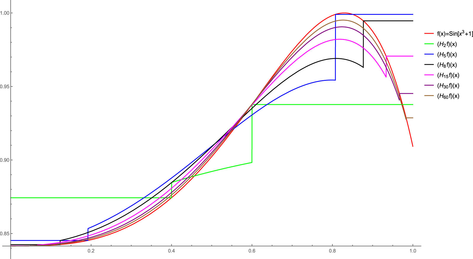
In the graphs below, the graphs of the different values of n of the hypergeometric operator sequence are expressed in different colors and are indicated next to the graph.

In addition, we give numerical tables for comparison between Bernstein and hypergeometric operators at some points.

Example 1

Let us consider the operator f ( x ) = x 5 , and we take its corresponding hypergeometric operator ( H n f ) ( x ) as r n = n 2 + 1 , then one has

The evaluation for comparison between Bernstein and hypergeometric operators at some points yield numerically, for n = 10 , 20 , and 40,

n = 10 n = 20 n = 40 ( H n f ) ( 0.3 ) 0.00984124 0.00575161 0.0039761 ( B n f ) ( 0.3 ) 0.0109222 0.00596114 0.00402021 f ( 0.3 ) 0.00243 0.00243 0.00243 ,

n = 10 n = 20 n = 40 ( H n f ) ( 0.5 ) 0.0633554 0.0471639 0.0391465 ( B n f ) ( 0.5 ) 0.066875 0.0480078 0.0393506 f ( 0.5 ) 0.03125 0.03125 0.03125 ,

n = 10 n = 20 n = 40 ( H n f ) ( 0.8 ) 0.400063 0.366051 0.347485 ( B n f ) ( 0.8 ) 0.406409 0.367857 0.347966 f ( 0.8 ) 0.32768 0.32768 0.32768 .

Example 2

Now, we consider the function f ( x ) = sin ( x 3 + 1 ) , then again for its corresponding hypergeometric operator ( H n f ) ( x ) as r n = n 2 + 1 , one has

Numerically, for n = 10 , 20 , and 40, we have

n = 10 n = 20 n = 40 ( H n f ) ( 0.3 ) 0.863464 0.859953 0.857941 ( B n f ) ( 0.3 ) 0.864157 0.860156 0.857995 f ( 0.3 ) 0.855751 0.855751 0.855751 ,

n = 10 n = 20 n = 40 ( H n f ) ( 0.5 ) 0.908374 0.906162 0.904457 ( B n f ) ( 0.5 ) 0.908705 0.906317 0.904507 f ( 0.5 ) 0.902268 0.902268 0.902268 ,

n = 10 n = 20 n = 40 ( H n f ) ( 0.8 ) 0.974208 0.985531 0.991698 ( B n f ) ( 0.8 ) 0.9723 0.984958 0.991542 f ( 0.8 ) 0.998272 0.998272 0.998272 .

Example 3

Let us finally consider the function f ( x ) = e x − x 2 , then again for its corresponding hypergeometric operator ( H n f ) ( x ) as again r n = n 2 + 1 , one has

As the reader will observe, also taking into account the numerical calculations, the H n f approximate to the function f in general somewhat better than B n f , at least for the particular functions f ( x ) = x 5 , f ( x ) = sin ( x 3 + 1 ) , as well as for f ( x ) = e x − x 2 .

Acknowledgement

I would like to thank the editor and referees for their careful reading and valuable suggestions that improved the quality and presentation of the paper.

Funding information: The author did not receive support from any organization for the submitted work.
Author contributions: The author confirms the sole responsibility for the conception of the study, presented results, and prepared the manuscript.
Conflict of interest: The author states that there is no conflict of interest.

References

[1] S. N. Bernstein, Demonstration du Thĕoreme de Weierstrass fondĕ sur le calcul des probabilitĕs, Comm. Soc. Math. 13 (1912/13), 1–2. Search in Google Scholar

[2] W. Meyer-Konig and K. Zeller, Bernsteinsche Potenzreihen, Studia Math. 19 (1960), 89–94. 10.4064/sm-19-1-89-94Search in Google Scholar

[3] D. D. Stancu, Approximation of functions by a new class of linear polynomial operators, Rev. Roumaine Math. Pures Appl. 13 (1968), 1173–1994. Search in Google Scholar

[4] V. Baskakov, An instance of a sequence of linear positive operators in the space of continuous functions, Dokl. Akad. Nauk SSSR 113 (1957), no. 2, 249–251. Search in Google Scholar

[5] O. Szász, Generalization of S. Bernsteinas polynomials to infinite interval, J. Res. Nat. Bur. Standards 45 (1959), 239–245. 10.6028/jres.045.024Search in Google Scholar

[6] G. Bleimann, P. L. Butzer, and L. Hahn, A Bernstein Type operator approximating continuous functions on the semi-axis, Indag. Math. 42 (1980), 255–262. 10.1016/1385-7258(80)90027-XSearch in Google Scholar

[7] F. Altomare and M. Campiti, Korovkin-Type Approximation Theory and its Applications, De Gruyter Studies in Mathematics, vol. 17, Walter de Gruyter and Co., Berlin, 1994. 10.1515/9783110884586Search in Google Scholar

[8] G. G. Lorentz, Bernstein Polynomials, University of Toronto Press, Toronto, 1953, 130 pp. Search in Google Scholar

[9] H. D. Brunk, J. E. Holstein, and F. Williams, A comparison of binomial approximations to the hypergeometric distribution, Amer Stat. 22 (1968), no. 1, 24–26. 10.1080/00031305.1968.10480437Search in Google Scholar

[10] A. N. Shiryayev, Probability, Springer-Verlag, NewYork, 1984. 10.1007/978-1-4899-0018-0Search in Google Scholar

[11] I. Chlodovsky, Sur le développement des fonctions définies dans un intervalle infini en séries de polynomes de M. S. Bernstein, Compositio Math. 4 (1937), 380–393. Search in Google Scholar

[12] H. Karsli, A complete extension of the Bernstein-Weierstrass Theorem to the infinite interval (−∞,+∞) via Chlodovsky polynomials, Adv. Oper. Theory 7 (2022), 15. 10.1007/s43036-021-00178-7Search in Google Scholar

[13] T. Kilgore, On a constructive proof of the Weierstrass theorem with a weight function on unbounded intervals, Mediterr. J. Math. 14 (2017), no. 6, Art. 217, 9 pp. 10.1007/s00009-017-1011-xSearch in Google Scholar

[14] P. P. Korovkin, Linear Operators and Approximation Theory, Hindustan Publishing Corporation, Delhi, 1960. Search in Google Scholar

[15] E. Voronovskaya, Détermination de la forme asymptotique daapproximation des fonctions par les polynômes de M. Bernstein, C. R. Acad. Sci. URSS 79 (1932), 79–85. Search in Google Scholar

Received: 2023-07-30

Revised: 2023-10-27

Accepted: 2023-11-13

Published Online: 2024-08-09

This work is licensed under the Creative Commons Attribution 4.0 International License.

Articles in the same Issue

https://doi.org/10.1515/dema-2023-0135

Keywords for this article

hypergeometric distribution; convergence; Korovkin theorem; modulus of continuity

Creative Commons

BY 4.0