A kind of univariate improved Shepard-Euler operators
-
Ruifeng Wu


Abstract
In this paper, a kind of univariate Shepard-Euler operators is studied by combining the known Shepard operator with the generalized Taylor polynomial as the expansion in the Euler polynomials. For practical purposes, another kind of improved Shepard-Euler operators without any derivative of the approximated function f is given by using divided differences to approximate the derivatives. Some error bounds and convergence rates of the combined operators are studied. Finally, some numerical experiments are shown to compare the approximation capacity of our operators with that of Caira-Dell’Accio’s scheme. Furthermore, there is no demand for the derivatives of f in the proposed operator, so it does not increase the orders of smoothness of f.
1 Introduction
The classical Shepard operator, first introduced in [1], is a well suited operator for two-dimensional interpolation of very large scattered data sets. Let f be a real valued function defined on
where
and |⋅| denotes the Euclidean norm in
and
Because S N,μ [f](x) reproduces only constant functions, so Shepard has suggested to apply S N,μ [f](x) not directly to the f(x i ), but to the Taylor polynomial of f of degree 1 at x i . In this case the combined operator has the degree of exactness 1 in [1].
To increase the degree of exactness of the Shepard operator, several combined operators have been introduced and studied on Taylor [1], [2], [3], [4], [5], Lagrange [6], Hermite [7], Birkhoff [8], and Bernoulli [9]. The Shepard method can also refer to recent developments on the subject, see [10], [11], [12], [13], [14], [15], [16] for details.
Based on the idea in [9], we first combine the Shepard operator S
N,μ
[f](x) in [1] with the generalized Taylor polynomial, the Euler-based expansion as one instance of two-point generalized Taylor polynomials introduced in [17] to obtain a kind of Shepard-Euler operators. The proposed Shepard-Euler operator
The organization of the remainder of this paper is as follows. In Section 2, we recall the definition of univariate Euler polynomials and give three useful theorems for the error of approximation that will be used later in the paper. In Section 3, we apply the previous results to derive a kind of Shepard-Euler operators with derivatives, and prove their convergence rates. In Section 4, another kind of improved Shepard-Euler operators without derivatives is provided. In Section 5, numerical examples are shown to demonstrate the accuracy of the proposed combination in some special situations. In Section 6, we give the main conclusions.
2 Some remarks about the generalized Taylor polynomial
The generalized Taylor polynomial is an expansion in the Euler polynomials E n (x), i.e., the polynomials of the sequence defined recursively by means of the following relations, see [19]
For functions in the class C
m
([a, b]),
where the polynomial expansion
and the remainder term
where
with h = b − a. The polynomial approximant
where T
m
[f; a](x) is the mth Taylor polynomial of f about a. Therefore, the expansion
To obtain bounds for the remainder
where f ∈ C m [c, d] with c < a and b < d. By using the Peano’s kernel theorem [20], we provide the integral expression for the remainder (8) as follows.
Theorem 1.
Let f ∈ C m [c, d] and x ∈ [c, d], then for the remainder
we have the following integral representations
where
and
Proof.
On the one hand, in the polynomial approximation term (7) there are evaluations of derivatives of f up to the order m on points a and b of [c, d]; on the other hand, the exactness of the polynomial approximant (9) on the space
where (13) is given by applying the linear functional
If t ∈ [c, x], then
where (x − t) m−1 is considered as a polynomial in x of degree m − 1.
If t ∈ [b, d], then
Thus, we now have proven the first case of (12). The remaining cases of (12) can be proved in an analogous manner.□
By Theorem 1, we can obtain the following result.
Theorem 2.
If f ∈ C m [c, d] and x ∈ [c, d], then for the remainder we have
where ‖ ⋅‖∞ denotes the sup-norm on [c, d] and
Proof.
Let c < x < a, then we have from the first case of (12) that
Let x < t < a, then
so that
Note that the integrands are of type h(t)f (m)(t) with a h(t) that does not change sign in [x, a]. By applying the first mean value theorem for integrals, we find for some ξ k ∈ [c, d], k = 0, 1, …, m, that
If a < t < b, then
and
Based on the first mean value theorem for integrals, we get for some β k , ∈ [c, d], k = 0, 1, …, m, that
Substituting into (20) the left-land sides of (22), (24) with their respective right-hand sides, we finally give after some calculations
and
In [21], we have the following known identity:
From the relations (25) we can easily deduce the following formula:
so that we get
Similarly, we can prove the remaining expressions of (18).□
Since the algebraic degree of exactness of the operator
Theorem 3.
If f ∈ C m+1[c, d] and x ∈ [c, d], then for the remainder we have
where
3 A kind of Shepard-Euler operators with derivatives
Suppose that x
1 < x
2 < … < x
N−1 < x
N
are fixed points in an interval
where
Theorem 4.
The operator
Proof.
The argument
and
where
To study the convergence rates of the two kinds of operators
where X = {x
1, x
2, …, x
N
} and #(⋅) denotes the cardinality function. So M denotes the maximum number of points from X contained in an interval I
r
(x). For the operators
Theorem 5.
Let f(x) ∈ C m (I). Then
where
C ⟨E⟩ is a positive constant independent of x, and X, and r is given above.
Proof.
Assume that each pair x i , x i+1 ∈ I is fixed and suppose x i < x i+1. For each x ∈ I, we make use of the following settings
Based on (2) and (30), we obtain
where
From [9], we can give the following prove:
Suppose that
where the set
where j = 2, 3, …, n and τ i ∈ [x i−1, x i+1]. Therefore, we find from (34)
On the other hand, we also find from the definition of M
Let us denote by x d the node closest to x i since
By applying (36) and (37), we have
where the last inequality follows from
Case 1: (μ > 1)
If 1 < μ < m + 1, then
If μ = m + 1, then
If μ > m + 1, then
Case 2: ( μ = 1)
□
In an analogous manner we can prove the following theorem.
Theorem 6.
Let f(x) ∈ C m+1(I). Then
where
and C ⟨E⟩ is a positive constant independent of x and X.
Because of disadvantage with the derivatives in the operator
4 A kind of improved Shepard-Euler operators without derivatives
Although the operator
Definition 1
(see [18]). Let
There exists a real vector
(41)For any
(42)
In such situation, we also say that
Suppose that |⋅| denotes the number of elements in set and assume that the points in set A are distinct, and |A| = m + 1. Then by Definition 1 and [18], a
where
According to the location of each pair x
i
, x
i+1 (i = 1, 2, …, N), we choose suitable sets A
i
, and substitute f
(k)(x
i
), f
(k)(x
i+1) in (30) by
Theorem 7.
The operator
Proof.
Since
so that
According to (46) and the proof of Theorem 4, we can obtain
For the Shepard-Euler univariate operator
Theorem 8.
Let f(x) ∈ C m+1(I). Then
where
and
Proof.
Consider
The first term of the right-hand sides in (49) has been obtained from the Theorem 6:
where
Based on (36) and (37), we get
Next, we need to prove the first term of the right-hand sides in (49). We denote by r
max, r
min the maximum and the minimum distance between adjacent nodes respectively. Let
Therefore, we have
and
Let
By applying (36) and (37), we have
By applying formulas (50), (52), and the results above, we can obtain
Case 1: (μ > 1)
If 1 < μ < m + 2, then
If μ = m + 2, then
If μ > m + 2, then
Case 2:(μ = 1)
□
5 Numerical examples
5.1 Verification of approximation capacity
We consider the following functions on the interval [0,1]:
These functions were first introduced in [9] and result from adapting to the univariate case test functions generally used in the multivariate interpolation of large sets of scattered data in [22]. For each function f
i
, i = 1, 2, …, 6 we will compare the numerical results of our new operators
We adopt uniform grids of 17 points for
Saddle.
| (μ, m) |
|
|
|
|||
|---|---|---|---|---|---|---|
| ɛ mean | ɛ max | ɛ mean | ɛ max | ɛ mean | ɛ max | |
| (2,1) | 0.001050 | 0.004954 | 0.001067 | 0.005139 | 0.001050 | 0.004955 |
| (2,2) | 0.001062 | 0.004715 | 0.001100 | 0.004430 | 0.001004 | 0.003710 |
| (2,3) | 0.001490 | 0.005153 | 0.001516 | 0.005141 | 0.001771 | 0.007104 |
| (3,1) | 0.000476 | 0.003314 | 0.000496 | 0.003220 | 0.000477 | 0.003315 |
| (3,2) | 0.000333 | 0.002302 | 0.000313 | 0.001076 | 0.000280 | 0.001071 |
| (3,3) | 0.000206 | 0.001096 | 0.000391 | 0.001568 | 0.000550 | 0.003165 |
| (4,1) | 0.000457 | 0.003233 | 0.000476 | 0.003158 | 0.000457 | 0.003234 |
| (4,2) | 0.000259 | 0.001908 | 0.000259 | 0.001042 | 0.000295 | 0.001007 |
| (4,3) | 0.000136 | 0.001460 | 0.000358 | 0.001649 | 0.000505 | 0.003001 |
Sphere.
| (μ, m) |
|
|
|
|||
|---|---|---|---|---|---|---|
| ɛ mean | ɛ max | ɛ mean | ɛ max | ɛ mean | ɛ max | |
| (2,1) | 0.002145 | 0.005623 | 0.002151 | 0.005592 | 0.002145 | 0.005624 |
| (2,2) | 0.000312 | 0.000842 | 0.000326 | 0.000839 | 0.000222 | 0.000534 |
| (2,3) | 0.000586 | 0.002344 | 0.000583 | 0.002392 | 0.000176 | 0.000888 |
| (3,1) | 0.000583 | 0.001620 | 0.000586 | 0.001576 | 0.000584 | 0.001620 |
| (3,2) | 0.000058 | 0.000247 | 0.000825 | 0.000171 | 0.000056 | 0.000198 |
| (3,3) | 0.000079 | 0.000323 | 0.000082 | 0.000315 | 0.000055 | 0.000167 |
| (4,1) | 0.000510 | 0.001447 | 0.000513 | 0.001512 | 0.000510 | 0.001448 |
| (4,2) | 0.000039 | 0.000255 | 0.000044 | 0.000171 | 0.000053 | 0.000209 |
| (4,3) | 0.000025 | 0.000113 | 0.000039 | 0.000130 | 0.000063 | 0.000195 |
Cliff.
| (μ, m) |
|
|
|
|||
|---|---|---|---|---|---|---|
| ɛ mean | ɛ max | ɛ mean | ɛ max | ɛ mean | ɛ max | |
| (2,1) | 0.006604 | 0.038815 | 0.006867 | 0.041552 | 0.006604 | 0.038816 |
| (2,2) | 0.004710 | 0.031367 | 0.005681 | 0.032557 | 0.005213 | 0.042274 |
| (2,3) | 0.013455 | 0.062821 | 0.019834 | 0.067441 | 0.012252 | 0.084868 |
| (3,1) | 0.002522 | 0.021627 | 0.002466 | 0.023453 | 0.002523 | 0.021627 |
| (3,2) | 0.002466 | 0.027527 | 0.002539 | 0.020448 | 0.003466 | 0.028998 |
| (3,3) | 0.002138 | 0.016732 | 0.008360 | 0.049557 | 0.009664 | 0.072554 |
| (4,1) | 0.002405 | 0.021752 | 0.002307 | 0.021369 | 0.002406 | 0.021753 |
| (4,2) | 0.002170 | 0.034048 | 0.002481 | 0.021815 | 0.003451 | 0.028254 |
| (4,3) | 0.001542 | 0.024101 | 0.007482 | 0.049916 | 0.009573 | 0.071607 |
Gentle.
| (μ, m) |
|
|
|
|||
|---|---|---|---|---|---|---|
| ɛ mean | ɛ max | ɛ mean | ɛ max | ɛ mean | ɛ max | |
| (2,1) | 0.002590 | 0.007116 | 0.002585 | 0.007136 | 0.002591 | 0.007116 |
| (2,2) | 0.001897 | 0.005956 | 0.001897 | 0.005475 | 0.001640 | 0.004237 |
| (2,3) | 0.001138 | 0.006015 | 0.000982 | 0.005419 | 0.000096 | 0.009007 |
| (3,1) | 0.000681 | 0.003277 | 0.000695 | 0.003216 | 0.000681 | 0.003278 |
| (3,2) | 0.000378 | 0.001727 | 0.000355 | 0.001089 | 0.000290 | 0.000703 |
| (3,3) | 0.000175 | 0.000940 | 0.000174 | 0.000854 | 0.000376 | 0.001751 |
| (4,1) | 0.000618 | 0.002978 | 0.000630 | 0.002926 | 0.000618 | 0.002979 |
| (4,2) | 0.000270 | 0.001163 | 0.000257 | 0.000606 | 0.000279 | 0.000622 |
| (4,3) | 0.000089 | 0.000575 | 0.000162 | 0.000425 | 0.000329 | 0.000983 |
Steep.
| (μ, m) |
|
|
|
|||
|---|---|---|---|---|---|---|
| ɛ mean | ɛ max | ɛ mean | ɛ max | ɛ mean | ɛ max | |
| (2,1) | 0.002358 | 0.012532 | 0.002542 | 0.013477 | 0.002359 | 0.012532 |
| (2,2) | 0.002950 | 0.015868 | 0.003583 | 0.013701 | 0.003489 | 0.011714 |
| (2,3) | 0.004950 | 0.019728 | 0.004996 | 0.022482 | 0.004876 | 0.018069 |
| (3,1) | 0.001930 | 0.011016 | 0.002034 | 0.010647 | 0.001930 | 0.011016 |
| (3,2) | 0.001501 | 0.009079 | 0.001521 | 0.004408 | 0.001338 | 0.004893 |
| (3,3) | 0.000909 | 0.005278 | 0.002128 | 0.007668 | 0.003780 | 0.012462 |
| (4,1) | 0.001945 | 0.011413 | 0.002014 | 0.010619 | 0.001945 | 0.014433 |
| (4,2) | 0.001323 | 0.008184 | 0.001322 | 0.004414 | 0.001390 | 0.004782 |
| (4,3) | 0.000815 | 0.006381 | 0.002138 | 0.006357 | 0.003766 | 0.012590 |
Exponential.
| (μ, m) |
|
|
|
|||
|---|---|---|---|---|---|---|
| ɛ mean | ɛ max | ɛ mean | ɛ max | ɛ mean | ɛ max | |
| (2,1) | 0.007669 | 0.034757 | 0.008035 | 0.036003 | 0.007670 | 0.034958 |
| (2,2) | 0.005271 | 0.025436 | 0.008158 | 0.026378 | 0.007703 | 0.030519 |
| (2,3) | 0.025296 | 0.067861 | 0.022226 | 0.059885 | 0.019342 | 0.072922 |
| (3,1) | 0.005122 | 0.021099 | 0.005439 | 0.022252 | 0.005123 | 0.021100 |
| (3,2) | 0.004379 | 0.024620 | 0.005992 | 0.015731 | 0.006238 | 0.020148 |
| (3,3) | 0.003523 | 0.020488 | 0.015247 | 0.058286 | 0.017772 | 0.046858 |
| (4,1) | 0.005026 | 0.022762 | 0.005276 | 0.021013 | 0.005026 | 0.022762 |
| (4,2) | 0.004233 | 0.024080 | 0.005834 | 0.015174 | 0.006435 | 0.019645 |
| (4,3) | 0.003020 | 0.018326 | 0.015702 | 0.058286 | 0.017589 | 0.043494 |
In Figure 1, we plot the absolute error graphs of
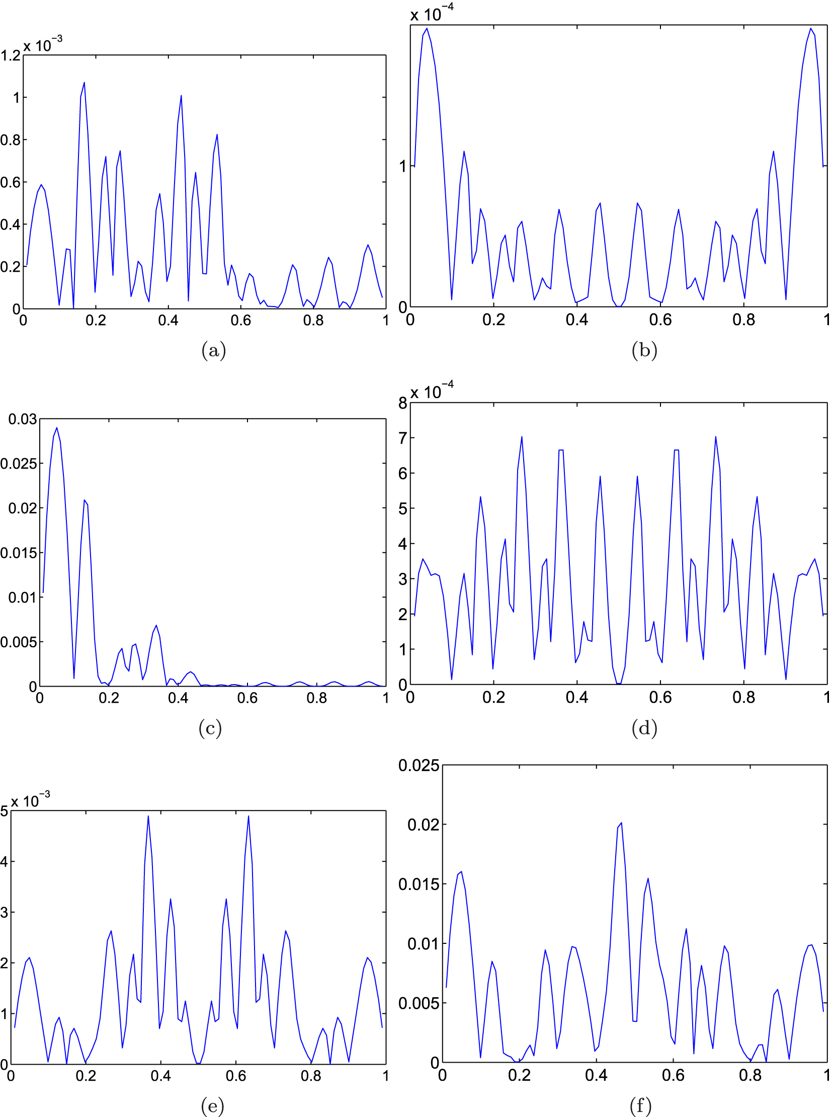
Absolute error graphs using operator
5.2 Comparison of computational cost
Suppose that Exponential. f
6(x) is still the approximated function, then we choose the different shape parameter μ and different positive integer m to compare the computational cost of our operators
Computational time(s) of the max errors of operators approximating f 6 as m = 2.
| (μ, m) | (2, 2) | (3, 2) | (4, 2) |
|---|---|---|---|
|
|
21.023985 | 21.106101 | 21.276911 |
|
|
42.213025 | 42.838780 | 44.621109 |
|
|
0.146423 | 0.124507 | 0.105130 |
Computational time(s) of the max errors of operators approximating f 6 as m = 3.
| (μ, m) | (2, 3) | (3, 3) | (4, 3) |
|---|---|---|---|
|
|
31.562475 | 30.887780 | 32.220974 |
|
|
47.240185 | 47.940174 | 47.033827 |
|
|
0.202907 | 0.248268 | 0.217616 |
From Tables 7 and 8, we find that for the different μ and m, our Shepard-Euler operator
6 Conclusions
In this paper, a kind of univariate Shepard-Euler operators
In the following work, on the one hand, we want to use it to the fitting of discrete solutions of the initial value problems of ODEs. On the other hand, the univariate Shepard-Euler operators can be extended to the multivariate case.
-
Research ethics: Not applicable.
-
Informed consent: Not applicable.
-
Author contributions: The author confirms the sole responsibility for the conception of the study, presented results and manuscript preparation.
-
Use of Large Language Models, AI and Machine Learning Tools: None declared.
-
Conflicts of interest: The author declares that he has no conflict of interest.
-
Funding information: This research was supported by the Science and Technology Research Projects of the Education Office of Jilin Province (Grant no. JJKH20250755KJ), the School Level Projection of Jilin University of Finance and Economics (Grant no. 2023YB024) and the BoYan PeiYou Special Projection of Jilin University of Finance and Economics (Grant no. 2024PY022).
-
Data availability statement: Data sharing is not applicable to this article as no datasets were generated or analyzed during the current study.
References
[1] D. Shepard, A two-dimensional interpolation function for irregularly-spaced data, Proceedings of the 23rd ACM National Conference, 1968, pp. 517–524.10.1145/800186.810616Suche in Google Scholar
[2] G. Coman and L. Ţâmbulea, A Shepard-Taylor approximation formula, Studia Univ. Babes-Bolyai Math. 33 (1998), 65–73.Suche in Google Scholar
[3] G. Coman and R. T. Trîmbiţaş, Combined Shepard univariate operators, East J. Approx. 7 (2001), no. 4, 471–483.Suche in Google Scholar
[4] B. Della Vecchia and G. Mastroianni, On functions approximation by shepard-type operators – a survey, in: S. P. Singh (ed.), Approximation Theory, Wavelets and Applications, Kluwer Academic Publishers, Dordrecht, 1995, pp. 335–346.10.1007/978-94-015-8577-4_20Suche in Google Scholar
[5] R. Farwig, Rate of convergence of Shepard’s global interpolation formula, Math. Comp. 46 (1986), no. 174, 577–590, https://doi.org/10.1090/S0025-5718-1986-0829627-0.Suche in Google Scholar
[6] G. Coman and R. T. Trîmbiţaş, Shepard operators of Lagrange-type, Studia Univ. Babes-Bolyai Math. 42 (1997), no. 1, 75–83.Suche in Google Scholar
[7] G. Coman, Hermite-type Shepard operators, Rev. Anal. Numér. Théor. Approx. 26 (1997), no. 1–2, 33–38.Suche in Google Scholar
[8] G. Coman, Shepard operators of Birkhoff-type, Calcolo 35 (1998), no. 4, 197–203, https://doi.org/10.1007/s100920050016.Suche in Google Scholar
[9] R. Caira and F. Dell’Accio, Shepard-Bernoulli operators, Math. Comp. 76 (2007), no. 257, 299–321, https://doi.org/10.1090/S0025-5718-06-01894-1.Suche in Google Scholar
[10] F. Dell’Accio and F. Di Tommaso, Bivariate Shepard-Bernoulli operators, Math. Comput. Simulation 141 (2017), 65–82, https://doi.org/10.1016/j.matcom.2017.07.002.Suche in Google Scholar
[11] F. Dell’Accio and F. Di Tommaso, On the hexagonal Shepard method, Appl. Numer. Math. 150 (2020), 51–64, https://doi.org/10.1016/j.apnum.2019.09.005.Suche in Google Scholar
[12] F. Dell’Accio, F. Di Tommaso, and E. Francomano, The enriched multinode Shepard collocation method for solving elliptic problems with singularities, Appl. Numer. Math. 205 (2024), 87–100, https://doi.org/10.1016/j.apnum.2024.07.005.Suche in Google Scholar
[13] O. Duman and B. Della Vecchia, Approximation to integrable functions by modified complex Shepard operators, J. Math. Anal. Appl. 512 (2022), no. 2, 126161, https://doi.org/10.1016/j.jmaa.2022.126161.Suche in Google Scholar
[14] O. Duman and B. Della Vecchia, Complex Shepard operators and their summability, Results Math. 76 (2021), no. 4, 214, https://doi.org/10.1007/s00025-021-01520-4.Suche in Google Scholar
[15] O. Duman, Shepard operators based on multivariable Taylor polynomials, J. Comput. Appl. Math. 437 (2024), 115456, https://doi.org/10.1016/j.cam.2023.115456.Suche in Google Scholar
[16] O. Duman and E. Erkus-Duman, Nonlinear approximation of vector valued functions by Shepard operators based on max-product and max-min operations, Fuzzy Sets and Systems 509 (2025), 109332, https://doi.org/10.1016/j.fss.2025.109332.Suche in Google Scholar
[17] F. A. Costabile and F. Dell’Accio, Polynomial approximation of CM functions by means of boundary values and applications: a survey, J. Comput. Appl. Math. 210 (2007), no. 1-2, 116–135, https://doi.org/10.1016/j.cam.2006.10.059.Suche in Google Scholar
[18] C. Rabut, Multivariate divided differences with simple knots, SIAM J. Numer. Anal. 38 (2001), no. 4, 1294–1311, https://doi.org/10.1137/S0036142999351042.Suche in Google Scholar
[19] G. Bretti and P. E. Ricci, Euler polynomials and the related quadrature rule, Georgian Math. J. 8 (2001), no. 3, 447–453, https://doi.org/10.1515/GMJ.2001.447.Suche in Google Scholar
[20] P. J. Davis, Interpolation and Approximation, Dover Publications, Inc., New York, 1975.Suche in Google Scholar
[21] H. Liu and W. Wang, Some identities on the Bernoulli, Euler and Genocchi polynomials via power sums and alternate power sums, Discrete Math. 309 (2009), no. 10, 3346–3363, https://doi.org/10.1016/j.disc.2008.09.048.Suche in Google Scholar
[22] R. J. Renka and A. K. Cline, A triangle-based C1 interpolation method, Rocky Mountain J. Math. 14 (1984), no. 1, 223–237, https://doi.org/10.1216/RMJ-1984-14-1-223.Suche in Google Scholar
© 2025 the author(s), published by De Gruyter, Berlin/Boston
This work is licensed under the Creative Commons Attribution 4.0 International License.
Artikel in diesem Heft
- On I-convergence of nets of functions in fuzzy metric spaces
- Special Issue on Contemporary Developments in Graphs Defined on Algebraic Structures
- Forbidden subgraphs of TI-power graphs of finite groups
- Finite group with some c#-normal and S-quasinormally embedded subgroups
- Classifying cubic symmetric graphs of order 88p and 88p 2
- Two-sided zero-divisor graphs of orientation-preserving and order-decreasing transformation semigroups
- Simplicial complexes defined on groups
- Further results on permanents of Laplacian matrices of trees
- Algebra
- Classes of modules closed under projective covers
- On the dimension of the algebraic sum of subspaces
- Green's graphs of a semigroup
- On an uncertainty principle for small index subgroups of finite fields
- On a generalization of I-regularity
- Algorithm and linear convergence of the H-spectral radius of weakly irreducible quasi-positive tensors
- The hyperbolic CS decomposition of tensors based on the C-product
- On weakly classical 1-absorbing prime submodules
- Equational characterizations for some subclasses of domains
- Algebraic Geometry
- Spin(8, ℂ)-Higgs bundles fixed points through spectral data
- Embedding of lattices and K3-covers of an Enriques surface
- Kodaira-Spencer maps for elliptic orbispheres as isomorphisms of Frobenius algebras
- Applications in Computer and Information Sciences
- Dynamics of particulate emissions in the presence of autonomous vehicles
- Exploring homotopy with hyperspherical tracking to find complex roots with application to electrical circuits
- Category Theory
- The higher mapping cone axiom
- Combinatorics and Graph Theory
- 𝕮-inverse of graphs and mixed graphs
- On the spectral radius and energy of the degree distance matrix of a connected graph
- Some new bounds on resolvent energy of a graph
- Coloring the vertices of a graph with mutual-visibility property
- Ring graph induced by a ring endomorphism
- A note on the edge general position number of cactus graphs
- Complex Analysis
- Some results on value distribution concerning Hayman's alternative
- Freely quasiconformal and locally weakly quasisymmetric mappings in metric spaces
- A new result for entire functions and their shifts with two shared values
- On a subclass of multivalent functions defined by generalized multiplier transformation
- Singular direction of meromorphic functions with finite logarithmic order
- Growth theorems and coefficient bounds for g-starlike mappings of complex order λ
- Refinements of inequalities on extremal problems of polynomials
- Control Theory and Optimization
- Averaging method in optimal control problems for integro-differential equations
- On superstability of derivations in Banach algebras
- The robust isolated calmness of spectral norm regularized convex matrix optimization problems
- Observability on the classes of non-nilpotent solvable three-dimensional Lie groups
- Differential Equations
- The ill-posedness of the (non-)periodic traveling wave solution for the deformed continuous Heisenberg spin equation
- A note on the global existence and boundedness of an N-dimensional parabolic-elliptic predator-prey system with indirect pursuit-evasion interaction
- Blow-up of solutions for Euler-Bernoulli equation with nonlinear time delay
- Periodic or homoclinic orbit bifurcated from a heteroclinic loop for high-dimensional systems
- Regularity of weak solutions to the 3D stationary tropical climate model
- Local minimizers for the NLS equation with localized nonlinearity on noncompact metric graphs
- Global existence and blow-up of solutions to pseudo-parabolic equation for Baouendi-Grushin operator
- Bubbles clustered inside for almost-critical problems
- Existence and multiplicity of positive solutions for multiparameter periodic systems
- Existence of positive periodic solutions for evolution equations with delay in ordered Banach spaces
- On a nonlinear boundary value problems with impulse action
- Normalized ground-states for the Sobolev critical Kirchhoff equation with at least mass critical growth
- Multiple positive solutions to a p-Kirchhoff equation with logarithmic terms and concave terms
- Infinitely many solutions for a class of Kirchhoff-type equations
- Real and non-real eigenvalues of regular indefinite Sturm–Liouville problems
- Existence of global solutions to a semilinear thermoelastic system in three dimensions
- Limiting profile of positive solutions to heterogeneous elliptic BVPs with nonlinear flux decaying to negative infinity on a portion of the boundary
- Morse index of circular solutions for repulsive central force problems on surfaces
- Differential Geometry
- On tangent bundles of Walker four-manifolds
- Pedal and negative pedal surfaces of framed curves in the Euclidean 3-space
- Discrete Mathematics
- Eventually monotonic solutions of the generalized Fibonacci equations
- Dynamical Systems Ergodic Theory
- Dynamical properties of two-diffusion SIR epidemic model with Markovian switching
- A note on weighted measure-theoretic pressure
- Pullback attractors for a class of second-order delay evolution equations with dispersive and dissipative terms on unbounded domain
- Pullback attractor of the 2D non-autonomous magneto-micropolar fluid equations
- Functional Analysis
- Spectrum boundary domination of semiregularities in Banach algebras
- Approximate multi-Cauchy mappings on certain groupoids
- Investigating the modified UO-iteration process in Banach spaces by a digraph
- Tilings, sub-tilings, and spectral sets on p-adic space
- Continuity and essential norm of operators defined by infinite tridiagonal matrices in weighted Orlicz and l∞ spaces
-
A family of commuting contraction semigroups on
- q-Stirling sequence spaces associated with q-Bell numbers
- Chlodowsky variant of Bernstein-type operators on the domain
- Hyponormality on a weighted Bergman space of an annulus with a general harmonic symbol
- Characterization of derivations on strongly double triangle subspace lattice algebras by local actions
- Fixed point approaches to the stability of Jensen’s functional equation
- Geometry
- The regularity of solutions to the Lp Gauss image problem
- Solving the quartic by conics
- Group Theory
- On a question of permutation groups acting on the power set
- A characterization of the translational hull of a weakly type B semigroup with E-properties
- Harmonic Analysis
- Eigenfunctions on an infinite Schrödinger network
- Maximal function and generalized fractional integral operators on the weighted Orlicz-Lorentz-Morrey spaces
- Subharmonic functions and associated measures in ℝn
- Mathematical Logic, Model Theory and Foundation
- A topology related to implication and upsets on a bounded BCK-algebra
- Boundedness of fractional sublinear operators on weighted grand Herz-Morrey spaces with variable exponents
- Number Theory
- Fibonacci vector and matrix p-norms
- Recurrence for probabilistic extension of Dowling polynomials
- Carmichael numbers composed of Piatetski-Shapiro primes in Beatty sequences
- The number of rational points of some classes of algebraic varieties over finite fields
- Classification and irreducibility of a class of integer polynomials
- Decompositions of the extended Selberg class functions
- Joint approximation of analytic functions by the shifts of Hurwitz zeta-functions in short intervals
- Fibonacci Cartan and Lucas Cartan numbers
- Recurrence relations satisfied by some arithmetic groups
- The hybrid power mean involving the Kloosterman sums and Dedekind sums
- Numerical Methods
- A modified predictor–corrector scheme with graded mesh for numerical solutions of nonlinear Ψ-caputo fractional-order systems
- A kind of univariate improved Shepard-Euler operators
- Probability and Statistics
- Statistical inference and data analysis of the record-based transmuted Burr X model
- Multiple G-Stratonovich integral in G-expectation space
- p-variation and Chung's LIL of sub-bifractional Brownian motion and applications
- Real Analysis
- Chebyshev polynomials of the first kind and the univariate Lommel function: Integral representations
- Multiple solutions for a class of fourth-order elliptic equations with critical growth
- Majorization-type inequalities for (m, M, ψ)-convex functions with applications
- The evaluation of a definite integral by the method of brackets illustrating its flexibility
- Some new Fejér type inequalities for (h, g; α - m)-convex functions
- Some new Hermite-Hadamard type inequalities for product of strongly h-convex functions on ellipsoids and balls
- Topology
- Unraveling chaos: A topological analysis of simplicial homology groups and their foldings
- A generalized fixed-point theorem for set-valued mappings in b-metric spaces
- On SI2-convergence in T0-spaces
- Generalized quandle polynomials and their applications to stuquandles, stuck links, and RNA folding