Exploring homotopy with hyperspherical tracking to find complex roots with application to electrical circuits
-
Mario A. Sandoval-Hernandez
 ,
Hector Vazquez-Leal
,
Hector Vazquez-Leal

Abstract
In the field of applied sciences, systems are frequently modeled using mathematical frameworks that include systems of nonlinear algebraic equations. Identifying their roots, whether real or complex, is of critical importance. The widespread use of complex numbers in science and engineering highlights the importance of accurately determining the complex roots of equations. This article presents a study in which the complex roots of a system of equations are identified through an approach that utilizes homotopy continuation, with the curve being traced using a hyperspherical path tracking technique. Furthermore, this article details five case studies on electrical networks where this method is applied to solve systems of equations containing imaginary coefficients to find mesh currents. The path tracking shows the behavior of system equation in each case study. Finally, an analysis of the precision of the solutions obtained in these case studies is provided, demonstrating an accuracy of up to 15 SDs in a single iteration during the refinement stage.
1 Introduction
In the history of complex numbers, a significant contribution was made by the mathematician Niccolò Tartaglia, who shared his secret solution techniques for solving equations with Girolamo Cardano, under the condition that Cardano would not disclose these techniques [1]. However, in 1545, Cardano published “Ars Magna”, a work in which he exposed methods for solving cubic equations [2,3]. This publication incited Tartaglia’s fury, as he accused Cardano of betrayal and dishonesty for failing to fulfill his promise. Nonetheless, Lodovico Ferrari, a young mathematician and Cardano’s assistant at the time, claimed that he was present during the meeting between the two mathematicians and asserted that no oath was taken [1].
Rafael Bombelli was familiar with the works of Girolamo Cardano on cubic equations, having studied his “Ars Magna”. However, he found some concepts therein to be confusing and believed it was possible to elucidate them, making the information more accessible to the general public. Bombelli embarked on the development of a formal algebra to handle expressions of the form
After the advancements made by Cardano and Bombelli, other mathematicians independently made significant contributions to the development of complex numbers. René Descartes, for instance, introduced the term “imaginary” in his work “La Géométrie” [5], marking the beginning of specific terminology to describe these numbers. On the other hand, John Wallis provided the first geometric interpretation of complex numbers, using line segments in the plane, which represented an important step toward their visual understanding [1].
Caspar Wessel, in his work “On the Analytical Representation of Direction: An Attempt Applied Chiefly to Solving Plane and Spherical Polygons” [6], demonstrated the geometric representation of an imaginary root of the form
Leonhard Euler standardized the notation for
In this context, considering the historical background, complex numbers are characterized by their arithmetic properties and various forms of representation, among them, the phasor [14,15]. These numbers are situated in the complex plane, where the abscissa axis represents the real part and the ordinate axis signifies the imaginary part [14,15]. Their application spans a wide range, covering several fields from mathematics to various engineering disciplines. A notable example of their use is found in fractals, which are geometric objects characterized by a basic structure that, whether fragmented or irregular, repeats at multiple scales. This concept was introduced by mathematician Benoît Mandelbrot in 1977, using the term “fractal” from the Latin “fractus”, meaning broken or fractured [16]. Among the most prominent fractal sets are the Mandelbrot and Julia sets, as highlighted by Monroy [14,17].
In the field of electricity and its subfields the applications of complex numbers have many applications, including the design of transmission lines in communications, where the Smith Chart is utilized for analyzing load impedances [18]. In signal processing, Fourier analysis employs the Fourier transform, which involves the imaginary expression in the exponential function’s argument, while the Fourier series in their complex form incorporates complex numbers [19]. In the qualitative theory of differential equations, the occurrence of complex roots in the eigenvalues of coefficient matrices plays a critical role in identifying behaviors such as centers and spirals, which can be stable or unstable [20]. In addition, in numerical analysis, complex numbers are utilized as starting points (SPs) in attraction basins to analyze the stability of numerical algorithms. They provide valuable information regarding the numerical instability of optimization methods, such as Newton-Raphson (N-R), the secant method, and Halley’s method, among others [21–23]. Various authors have developed numerous analytical techniques using attraction basins. For instance, in [24], algorithms were developed for plotting the basins of attraction of fixed-points for a pair of bivariate rational functions using toroidal attraction basins. Moreover, in optics, complex numbers are employed to apply Fresnel integrals in diffraction phenomena [25]. In electrodynamics, they facilitate the study of the reflection and transmission of electromagnetic waves [26]. In the field of antenna design and behavior, complex numbers are applied in analyzing parameters such as impedance measurements, polarization, near-field and electromagnetic analysis, among others [27]. In electrical circuits, complex numbers are fundamental for calculating capacitive and inductive reactances, enabling the analysis of AC circuits [15]. Similarly, in power electrical systems, including industrial motors, networks, and three-phase circuits, they play a crucial role [28]. Furthermore, complex numbers are essential in the analysis of stability and frequency response [29], as well as in electronics for the analysis and synthesis of active filters [30,31]. In engineering, systems are modeled by equations and systems of differential, and occasionally algebraic, equations. Understanding the solutions to these equations is crucial, as they reveal the behavior of the system under given conditions. Specifically, for algebraic equations, the solutions can sometimes be complex. However, when dealing with equations that have real coefficients, these complex solutions appear in conjugate pairs [32].
There are several methods to determine complex roots in polynomial algebraic equations. For example, [32] details the Graeffe method as a technique for finding all the roots of an equation, whether real or imaginary. The Jenkins-Traub method is a globally convergent numerical algorithm that can find the real and complex roots of polynomials of a single variable [33]. Sandoval-Hernandez et al. [34] proposed a hybrid perturbation-N-R method to solve a nonlinear algebraic equation (NAEs) in circuit analysis, specifically to determine the bias points of a tunnel diode using real solutions. Dubeau and Gnang [35] employed the fixed-point and N-R methods to find solutions to nonlinear equations in the complex plane. In [36], Newton’s method was adapted to polynomials with multiple roots in complex variables, applying it to Julia sets. On the other hand, Sandoval-Hernandez et al. [37] used a complex variable to obtain the general formula for solving quadratic equations. This formula is well known because it facilitates finding the different solutions of a quadratic equation, including solutions with complex numbers. In addition to the known methods for determining roots in equations, such as Regula Falsi or N-R, there are homotopy continuation algorithms that allow for solving systems of NAEs that can include transcendental functions. These are considered global convergence methods because they possess the ability to find solutions to nonlinear problems from almost any SP, theoretically ensuring that a solution will be reached regardless of the initial conditions. However, several authors have investigated the identification of complex roots through the application of homotopy continuation methods (HCMs). For instance, Gdawiec et al. [38] employed homotopy continuation for polynomial equations possessing both real and complex roots as a viable alternative to conventional iterative techniques. This approach was adopted to circumvent the issue of divergence.
In [39], an analysis was conducted on the SP utilizing the differential HCM to determine the conditions under which the convergence of these methods remains independent of the SP. This investigation aimed to facilitate the application of this technique to chemical engineering problems. However, the study also explored the behavior of the homotopic path in a case study where certain roots could not be identified due to the homotopic route encountering a region within the complex domain. Following this, in [40], the implementation of continuation homotopy was conducted to determine the roots of polynomial equations with real coefficients by substituting the complex variable
Due to its ability to find multiple roots in NAEs, homotopy has broad applications in chemical engineering. For example, chemical process control problems and chemical reactions often involve nonlinear equations with multiple solutions, heat diffusion processes, exothermic reaction, natural convection of air in a 2D square cavity at a steady state, and homotopic methods enable the identification of all possible solutions, allowing the selection of the most appropriate one [43–45], solution vectors for an elliptic system of 2D partial differential equations for natural convection [46]. Likewise, homotopy methods have been applied in electronic circuits to find the polarization point in nonlinear circuits [47,48,49], and in electronics to determine the operating point in circuits with transistors [50–56]. In addition, they have been used in the design of simulators for electronic circuits [57,58].
Recently, Vazquez-Leal and his research team [59] initiated a new line of research in robotics, emphasizing the importance of understanding the behavior of the homotopic path that models the movement trajectory of a mobile device. In [60], homotopy with hyperspherical tracking was applied for route planning, solving an NAE system that models the obstacles to be avoided. Furthermore, in [61,62], homotopy with hyperspherical tracking was utilized in a collision-free trajectory planning algorithm for robotic arms, addressing an NAE system that models the robot’s workspace.
This paper introduces the implementation of continuation homotopy with hyperspherical tracking [44,63], implemented in Maple using symbolic programming. This approach enables comprehensive tracking, considering both the real and imaginary parts integrally without their separation, aimed at resolving various systems of equations with imaginary coefficients within the context of electrical engineering problems. This method facilitates the exploration and examination of the solutions obtained, as well as the analysis of the behavior of their homotopic paths. Furthermore, it enhances the body of literature [64,65] dedicated to the determination of real roots of systems of equations through the use of continuation homotopy.
This paper is organized as follows: Section 2 introduces a brief historical note about continuation homotopy. Section 3 introduces the continuation homotopy method with hyperspherical tracking. Section 4 presents five case studies; the first involves a system of polynomial equations, while the subsequent case studies focus on solving systems of equations applied to electrical circuits. Section 5 details the numerical simulations and discussions. Finally, Section 6 outlines the conclusions of this work.
2 A brief historical review of HCMs
The formal origins of homotopy trace back to the work of French mathematician Henri Poincaré (1854–1912), widely regarded as the founder of algebraic topology. In his series of publications entitled “Analysis Situs”, Poincaré introduced the foundational concepts that would later develop into the theory of homotopy [66]. To fully contextualize the state of the art during Poincaré’s era, it is essential to understand the problem that sparked his interest in topology.
To understand the foundation of homotopy, it is essential to review the transformations involved. Topology studies the properties of geometric bodies that remain invariant under continuous transformations and their inverses [67]. This concept focuses on specific points that do not change when geometric bodies are contracted, expanded, or deformed [68,69]. In Figure 1, the points on the cube are relocated without generating new points during compression or expansion, illustrating a continuous transformation. This property, where
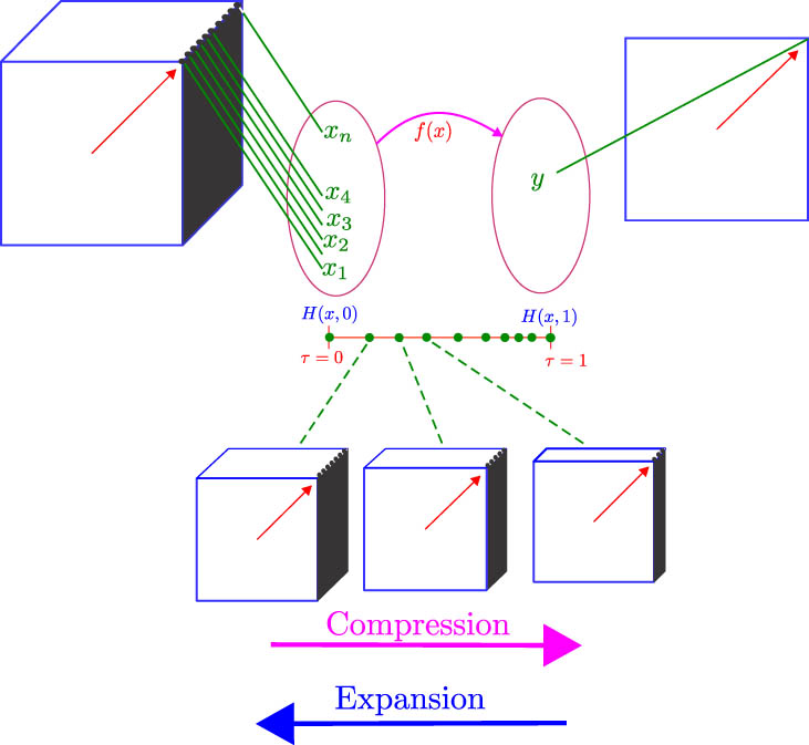
Schematic diagram of Homotopy between two geometric bodies.
Poincaré’s contributions to topology were of immense importance, as he introduced algebraic tools that enabled mathematicians to study abstract geometric properties without relying on classical geometric intuition. Homotopy became a cornerstone of this approach, offering an algebraic framework for addressing complex topological problems [70].
One of the first significant practical advances derived from homotopy theory was the fixed-point theorem, formulated by the Dutch mathematician Brouwer [72,73]. This theorem states that any continuous function mapping a closed sphere onto itself must have at least one fixed-point, meaning a point that remains invariant under the function. This theorem forms the philosophical link between Poincaré’s homotopy theory and the development of tools for solving algebraic equations and systems of equations. García and Zangwill further elaborate on the concept introduced by Brouwer [74].
In the context of homotopy theory, Brouwer’s theorem established a direct connection between the abstract concepts of algebraic topology and the solution of concrete problems in NAEs. This theorem marked homotopy’s first major application in developing methods for solving systems of equations, a line of research that would be extensively explored in the following decades [74].
As homotopy theory evolved, new tools were developed to tackle more complex problems. In 1934, French mathematicians Jean Leray and Jules Schauder introduced the concept of “topological degree” in their work “Topologie et équations fonctionnelles” as an extension of homotopy theory for systems of nonlinear equations [75]. The topological degree is an algebraic invariant that measures the “number of solutions” of a nonlinear equation by analyzing the signs of the derivatives or Jacobians of the functions involved.
The topological degree was crucial in formalizing HCMs. These methods involve continuously transforming a system of nonlinear equations into a simpler version with a known solution and then following this transformation until the solution of the original system is obtained. This is accomplished through a homotopic function, which links the solutions of the original system to those of the simplified system via the homotopic variable
In the 1950s, homotopy methods progressed with the development of corrector-predictor methods, proposed by Ficken in 1951 in his article “The Continuation Method for Functional Equations” [76]. These methods combined solution prediction with iterative correction using the N-R method to ensure convergence. One major improvement was the introduction of tangent predictors to the homotopic curve. In 1961, Haselgrove advanced this approach by applying Newton’s Method as a corrector in systems of nonlinear equations, detailed in his work “The Solution of Non-Linear Equations and of Differential Equations with Two-Point Boundary Conditions”, he details the use of Newton’s n-dimensional algorithm in the solution of systems of
Horizontal Predictors: Proposed by Lahaye in 1934 [79] and later used by Davidenko in 1953 [78,80], these methods sequentially increase the homotopy parameter. However, they are less efficient when there are returns along the homotopy path, as they require precise control of step size to ensure accuracy.
Differential Predictors: Introduced by Haselgrove in 1961 [77], they use the slope of the homotopic path to predict the next point to correct. Compared to horizontal predictors, they offer predictions closer to the actual path, facilitating convergence on local correction methods.
Polynomial Predictors: Proposed by Rheinboldt in 1975 [81], these methods use polynomial functions, such as Lagrange and Hermite polynomials, to predict the next point on the curve. Although they offer greater accuracy compared to earlier methods, their effectiveness decreases on curves with returns.
Closed Surfaces: The use of closed surfaces as predictors has had limited practical application in homotopy methods and was first introduced by Lyness and McHugh in 1963 [83]. They employed “hypercubes” in numerical integration, comparing their method to traditional techniques like Simpson and Euler-Maclaurin, showing improved precision [84]. After 1963, few publications have reported on closed trajectories as a prediction method for homotopy curves.
Hyperspherical Path Tracking: Jiménez-Islas reviewed the closed surface approach in 1985, conducting various analyses. He was the first to propose hyperspherical tracking ad hyperspherical tracking with variable radius in his 1988 master’s thesis, “Paquete Computacional para la Solución de sistemas de ecuaciones no lineales” [85], at Instituto Tecnológico de Celaya, without knowledge of Ushida’s work [86]. Islas published his results until 1996, applying them to chemical engineering [44].
On the other hand, since 1976, Ushida and Chua worked on solving nonlinear equations in circuit theory using continuation homotopy to address sharp turning points in solution curves [48,49]. In their 1984 article “Tracing Solution Curves of Nonlinear Equations with Sharp Turning Points” [86], they introduced an additional equation for homotopy formulation using arc-length. Previously, this idea had been used in other works [47–49,87].
The contribution in this article [86] was to solve the system of
From 1960s, homotopy methods advanced with the introduction of arc-length parameterization, proposed by Klopfenstein in 1961, which improved solution tracking and mitigated issues related to singularities in the Jacobian [91]. This technique provided greater control over curve tracking. In addition, homotopy methods faced challenges with bifurcations, where solution curves split into multiple branches, signaling changes in solution stability [92]. Alexander and Yorke generalize the HCM in “The Homotopy Continuation Method: Numerically Implementable Topological Procedures” [93], freeing it from its dependence on degree and broadening its application to problems beyond traditional degree arguments, particularly in locating bifurcating sets in nonlinear equations.
Homotopy methods have continued to evolve with the introduction of other techniques to improve their robustness and applicability. For example, Chow et al. [94] presented an approach based on a transversality theorem called “the Parametrized Sard Theorem”. This work gave solutions to problems in which the topological scheme is more complicated, for example, finding the Brouwer fixed-point, finding solutions of two point boundary problems for second-order ordinary differential equations in
Over time, various homotopy methods have been developed, including Newton homotopy [98], fixed-point homotopy [99,100], affine homotopy [84], Combined fixed-point Newton homotopy [101], probability one homotopy [102], and multiparameter homotopies [103]. In all cases, homotopies find a solution when the homotopic parameter
3 Basic concepts of HCMs
Solving systems of NAEs can be challenging using traditional approaches such as the N-R method. The N-R method requires an initial approximation of the solution to begin the process. However, it is well known that for some cases, the N-R method may not converge to a solution from any SP. Often, finding an appropriate initial guess is not straightforward or even feasible. As a result, the reliability of the N-R method for solving all types of problems cannot be assured. An alternative strategy to overcome this limitation involves employing HCM. The HCM methods represent a continuous deformation from a basic problem (easy to solve) to the target problem (difficult to solve), facilitating a smoother pathway to finding solutions.
HCMs are utilized to locate multiple solutions within systems of NAEs (
The HCMs introduce a perturbation in the system
where
Equation (2) represents any homotopy formulation that meets the following conditions:
If
If
The deformation process of the system initiates at
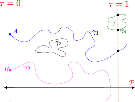
Family of homotopy curves.
The selection of
where
The application of HCM requires the implementation of a technique to map the homotopic path [44]. For example, when a hypersphere
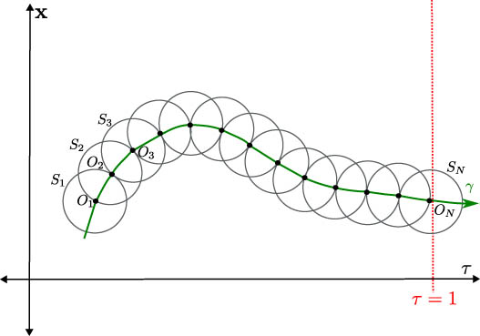
Potential homotopy path.
3.1 Path tracking of the homotopy trajectory
The formulation of a homotopy system involves
where
For the case of
During the tracking algorithm, the center of (4) must be updated at each tracking step and resolved for (5). Subsequently, spherical tracking is conducted, as depicted in Figure 3. Initially, we center the first hypersphere at the SP of the homotopy. Next, a prediction step is performed to approach the next point, and a correction step ensures the path following of the homotopy curve. Finally, the center of the hypersphere is updated at (5), and the process is repeated until the procedure reaches
The predictor-corrector scheme enables the spherical algorithm (SA) to accurately track the homotopy curve
where
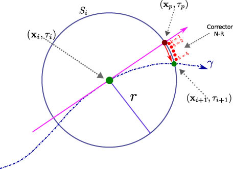
N-R corrector in spherical tracking.
The N-R method is used to correct the predictor point to a point on the homotopy path
where
3.2 Implementation of homotopy with spherical path tracking
The predictive section of the hyperspherical path tracking methodology presented in [44] forms the core of the strategy. The predictive homotopic path tracking is applied to a system of nonlinear equations derived from a set of
It is noteworthy that the addition of the parameter
By expressing equation (9) as a system of equations in its matrix form, we have
By applying Cramer’s rule in equation (10), we have the solution to the system
where
where
In this way, by rewriting (13) in the form of a column vector, a general expression for the slopes is obtained
Equation (14) expresses the slopes for each of the variables in the homotopic path
where
The sign will depend on the direction of tracking to the right or left, that is, in a positive or negative direction. In this way, it is possible to calculate the prediction for
Once the prediction vectors have been calculated, they now serve as the new initial values to begin the hyperspherical correction procedure, whose objective is to find the intersection between the hypersphere and the homotopic path, as shown in Figure 4. This procedure is carried out using the N-R method to solve the homotopic equations of the system, described by (3), and with the equation of the hypersphere (4). The N-R method, in two or more dimensions, requires the Jacobian matrix and a vector with the function evaluated at an initial point
However, it is possible to identify in
In order to generate the interpolated start points (ISPs) for FZS, the variables
3.3 Flowchart and pseudocode
Figure 5 illustrates the flowchart of the algorithm for homotopy with hyperspherical tracking. Each of the key points of the algorithm is summarized as follows:
The formulation of the system of homotopy equations is initiated by including the hypersphere equation.
Set the number of iterations for hyperspheres and initialize the counter.
Establish the nonsquare matrix
Proceed to calculate the predictor vector. The symbol
Apply N-R for homotopic correction. Save in a list
Calculate
Interpolate and apply N-R. Save the solutions in a list.
If the number of hypersphere iterations has been reached, print the solutions and the homotopic tracking.
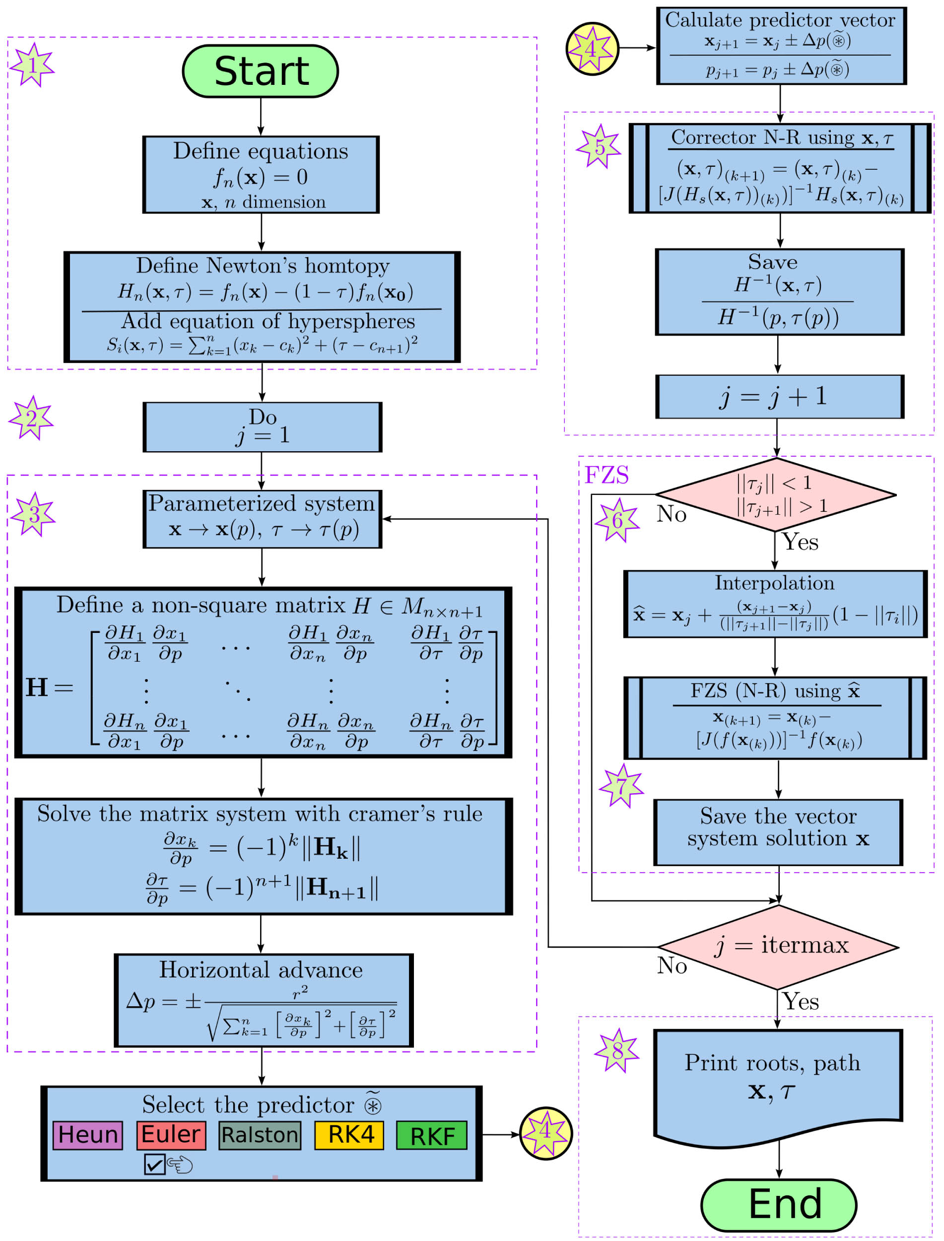
Flow chart for homotopy with hyperspherical tracking.
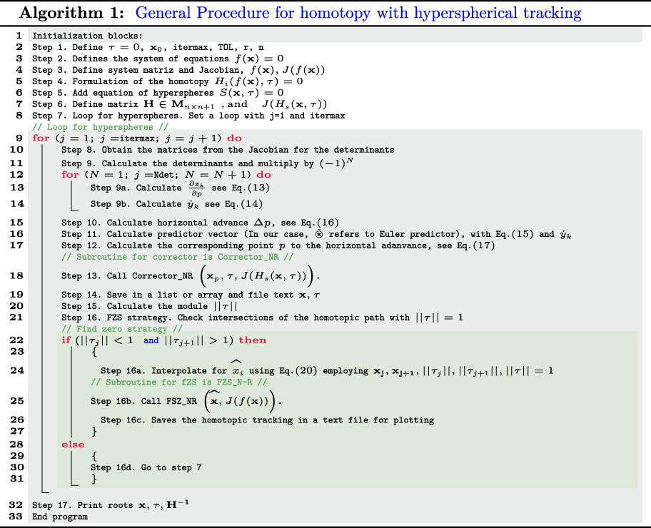
Algorithm 1 shows the pseudocode of the flowchart in Figure 5, where each necessary step for coding in programming languages such as Maple, Matlab, C++, Python, among others, is detailed. The presented pseudocode describes the implementation of the homotopy algorithm for hyperspherical tracking in a simplified manner, highlighting the main steps for its coding.
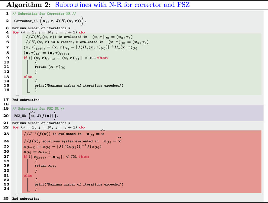
Algorithm 2 shows the pseudocode for the corrector_N-R subroutine of the flowchart in Figure 5. The subroutine receives as arguments the symbolic
4 Case studies
The mesh analyses presented in the case studies are fundamental in the analysis of circuits within electrical and electronic engineering. Both mesh and node analyses are important in the analysis of electrical circuits [28]. In electrical engineering, the relevance of mesh analysis is vast, being applied, for example, in three-phase circuits and those involving motors [28]. Furthermore, in the analysis of AC circuits, the frequencies of the voltage sources generate reactances in components such as capacitors and inductors. With passive devices such as capacitors and inductors, we obtain impedance, whose unit of measurement is the ohm [15,28,31].
Likewise, these analyses allow the application of various theorems, such as Thevenin’s theorem and the superposition theorem, among others, to simplify circuit analysis. In electronics, mesh analysis is essential for studying circuits with transistors, in both direct current and small signal analyses [108,109]. Transistors are the foundation of electronics and the design of analog integrated circuits, as well as integrated circuits of the transistor-transistor logic (TTL) and complementary metal-oxide-semiconductor (CMOS) families [108–110], microcontrollers [111], microprocessors [112], and others.
This section presents five case studies. The first involves a system of two algebraic simultaneous equations with real coefficients. The second and third case studies focus on mesh analysis of AC electrical circuits. In the fourth case study, the voltages of a small power system connected to a motor are determined. The final case study presents a mesh analysis of AC electrical circuits incorporating nonlinear impedances. In all case studies, we use the notation “j” for the imaginary part of the complex numbers, and the radius of the hyperspheres is
4.1 Case study 1
Solve the system of equations given by
This system of equations can be solved by algebraic or numerical methods. To solve it, in this work, two SPs were proposed to solve the system (21),
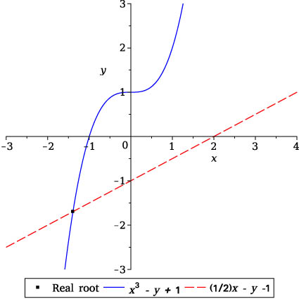
Plots for equations for case study 1.
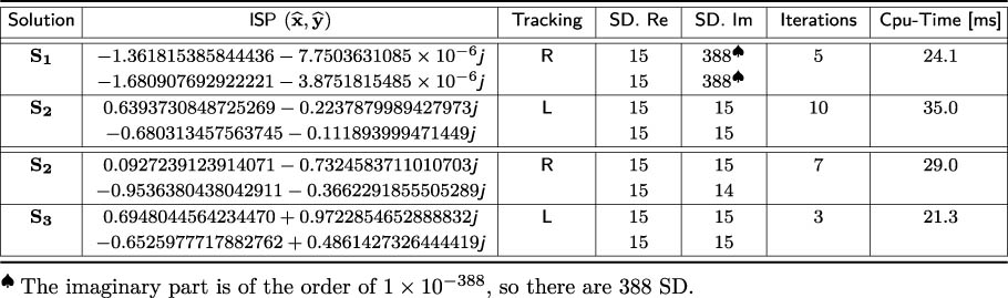
Table 1 summarizes the roots found with SPs used, the direction of the tracking, right (R) and left (L), the hypersphere iterations used, and CPU time in seconds. For example, the solutions
Homotopic tracking for case study 1
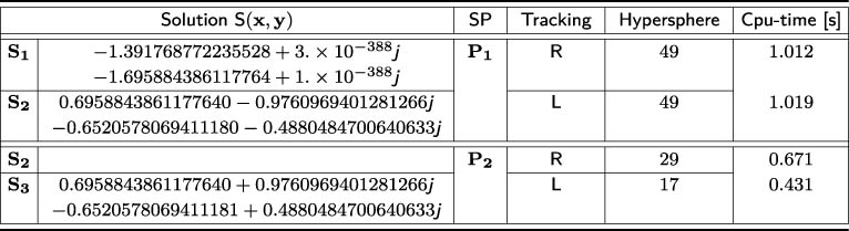 |
Figure 7 displays the homotopic tracking to find
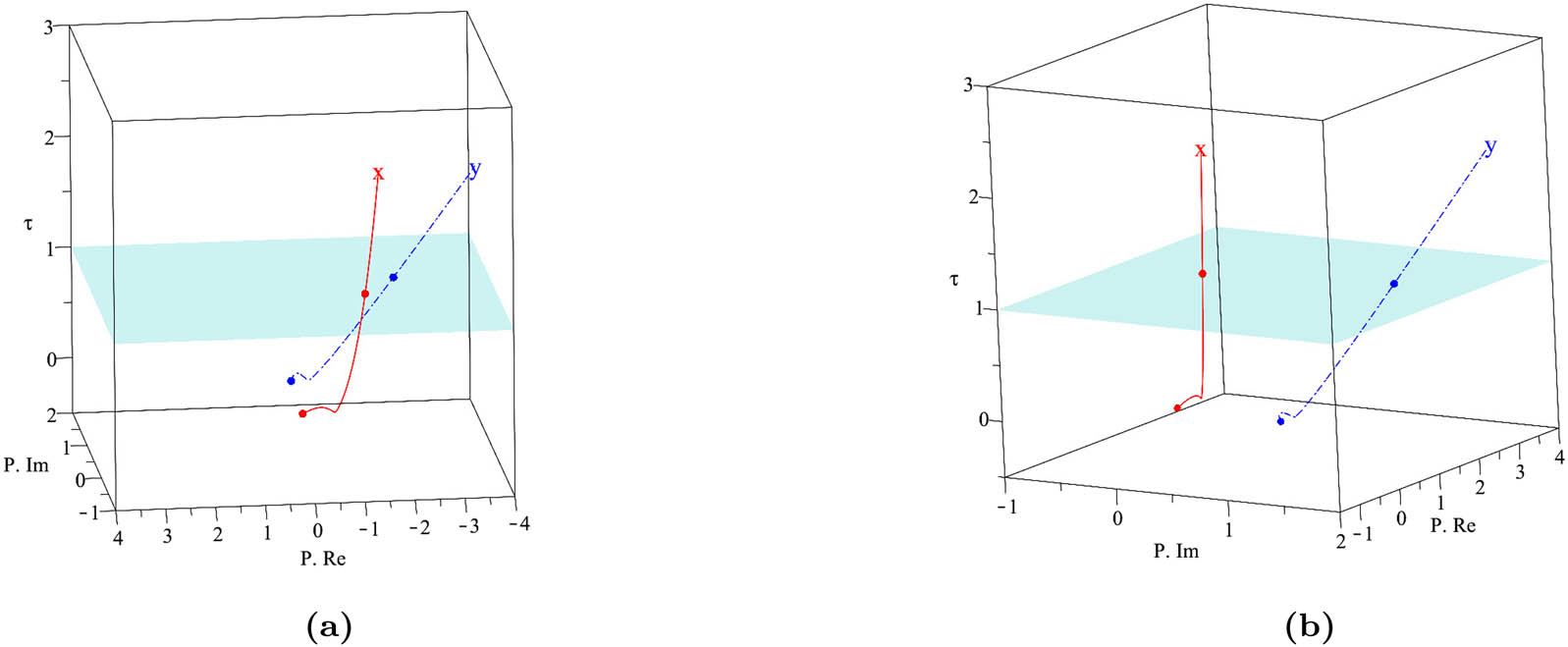
Hyperspheric homotopic tracking with
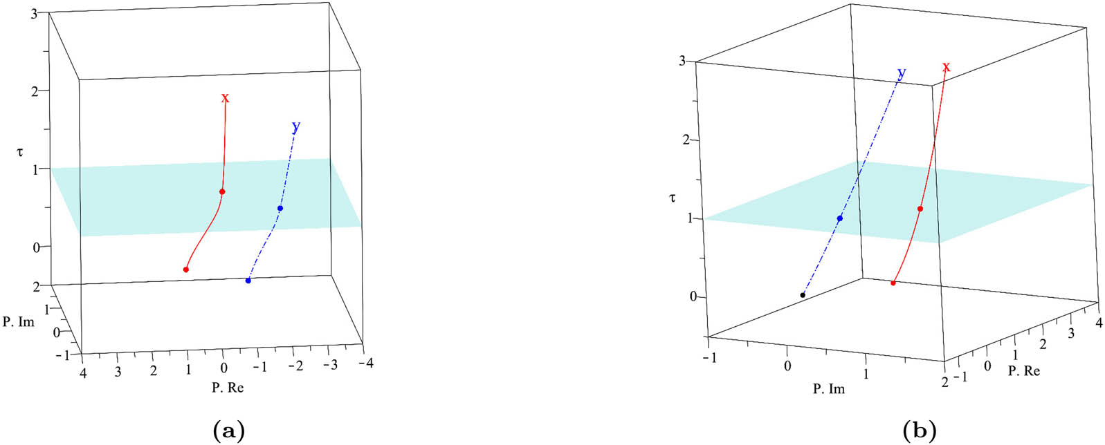
Hyperspheric homotopic tracking with
4.2 Case study 2
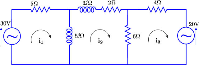
Find the mesh currents of the polarization point
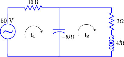
Electrical circuit with two meshes for case study 2.
This circuit was solved in [15] using Cramer’s rule. The loop equations of the circuit in Figure 9 were formulated with Kirchhoff’s law of charge conservation [15]. Therefore, the system of simultaneous equations of the circuit is given by
Unlike the system of equations presented in case study 1, the coefficients of (22) in this case study are complex. Applying homotopy with hyperspherical tracking to solve the system of simultaneous equations, a SP
Homotopic tracking for case study 2
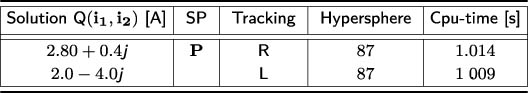 |
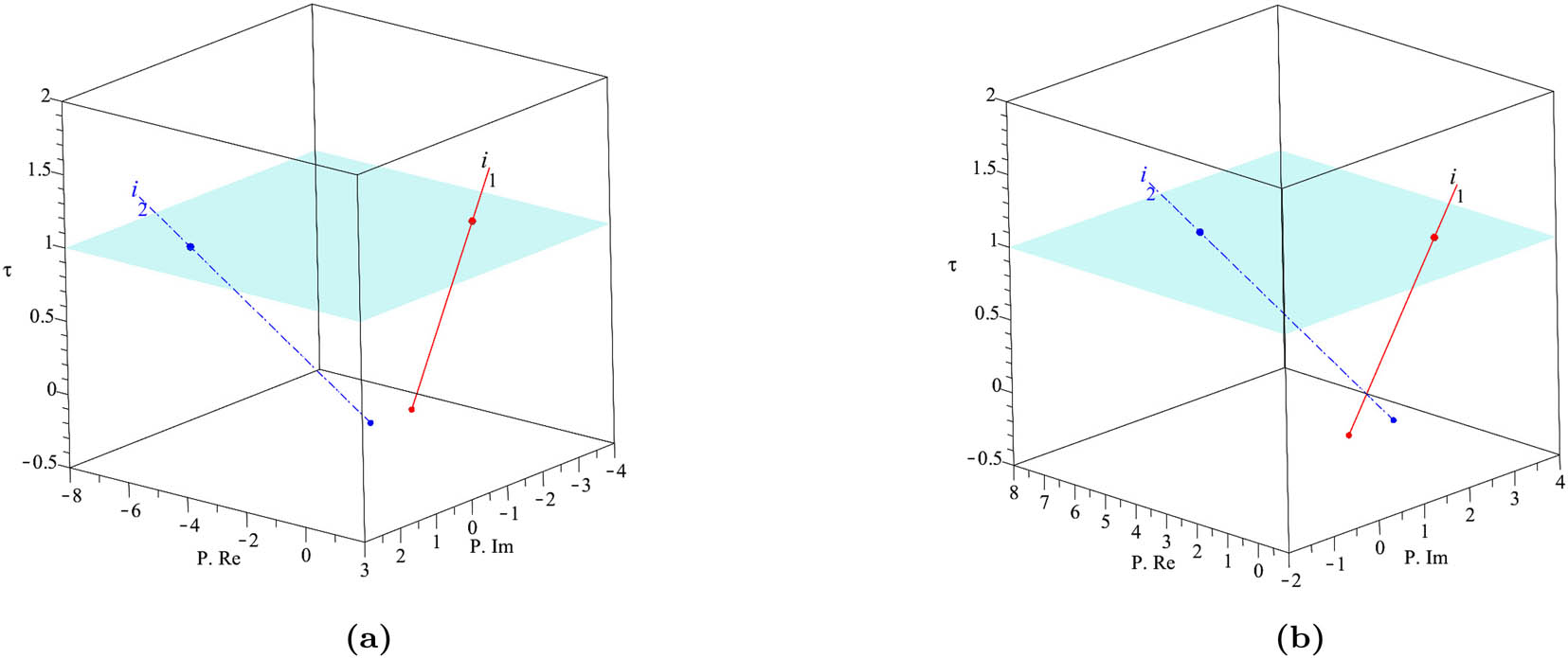
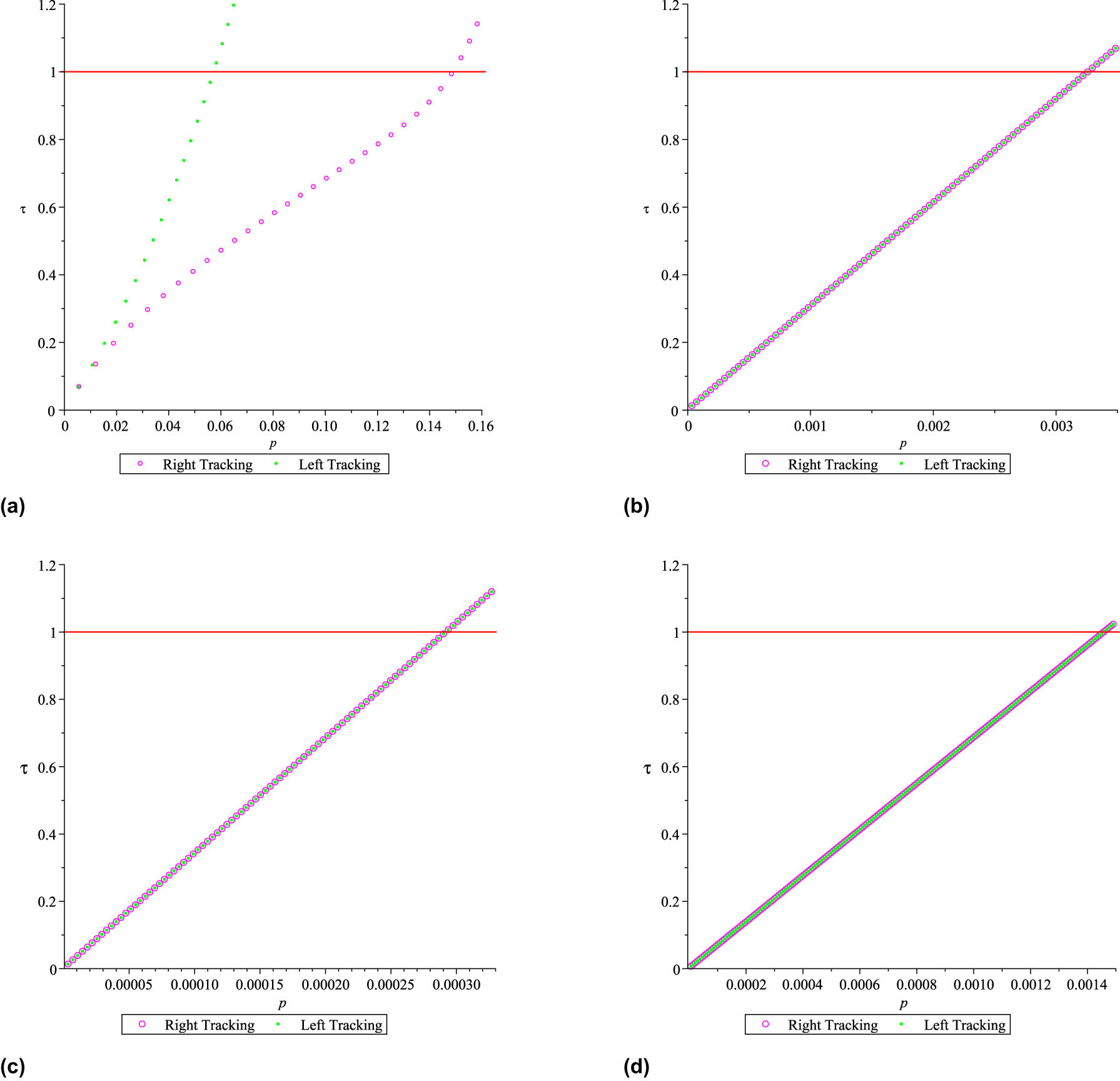
Figure 10 displays the homotopic tracking in both directions to determine solutions. Observe the linear behavior of the tracking paths for
Hyperspheric homotopic tracking with
4.3 Case study 3
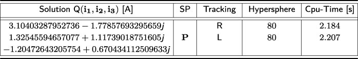
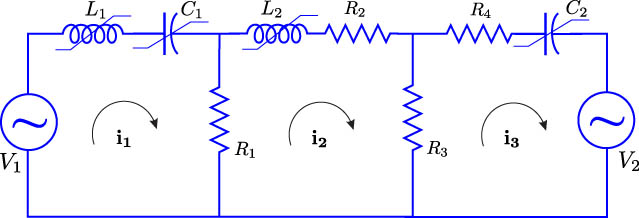
Find the mesh currents of the polarization point
Electrical circuit with three meshes for case study 3.
Likewise, this circuit was solved in [15] using the rule of Cramer. The loop equations for the circuit in Figure 11 are given by
Using the SP
Homotopic tracking for case study 3
 |
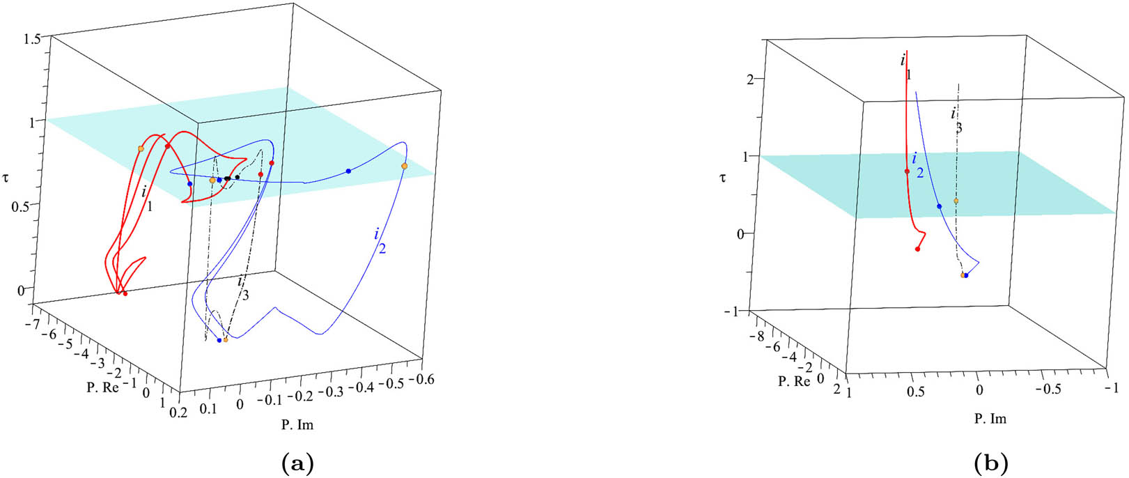
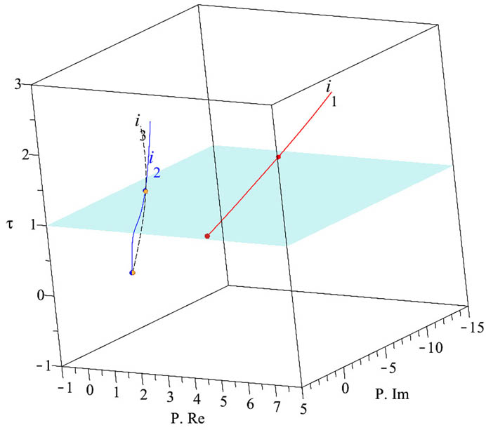
The behavior of the homotopic path exhibited by

Hyperspheric homotopic tracking with
4.4 Case study 4
In [28], the problem for the single-line diagram of a small power system shown in Figure 13 (a) was solved. The equivalent reactance diagram, with reactances, is shown in Figure 13 (b). A generator with an electromotive force equal to 125 [V] per unit is connected through a transformer to high-voltage node 3, while a motor with internal voltage equal to
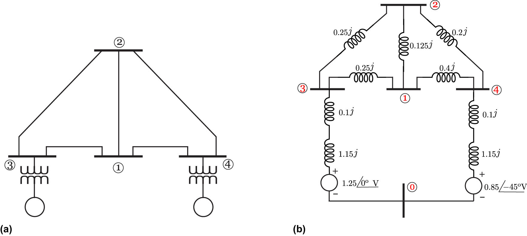
The single-line diagram of a small power system. (a) Single-line diagram of the four-bus system and (b) reactance diagram.
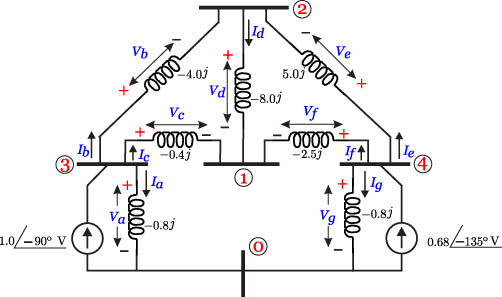
Electrical circuit with three meshes for case study 4.
Applying Kirchhoff’s voltage law, the node voltage equations for the equivalent of Figure 14 is given by (24)
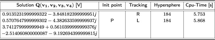
Using the SP
Homotopic tracking for case study 4
 |
Figures 15 (a) and (b) display the hyperspherical homotopic tracking with linear behavior for each of the voltages of the system equation (24), showing the unique solution in the plane
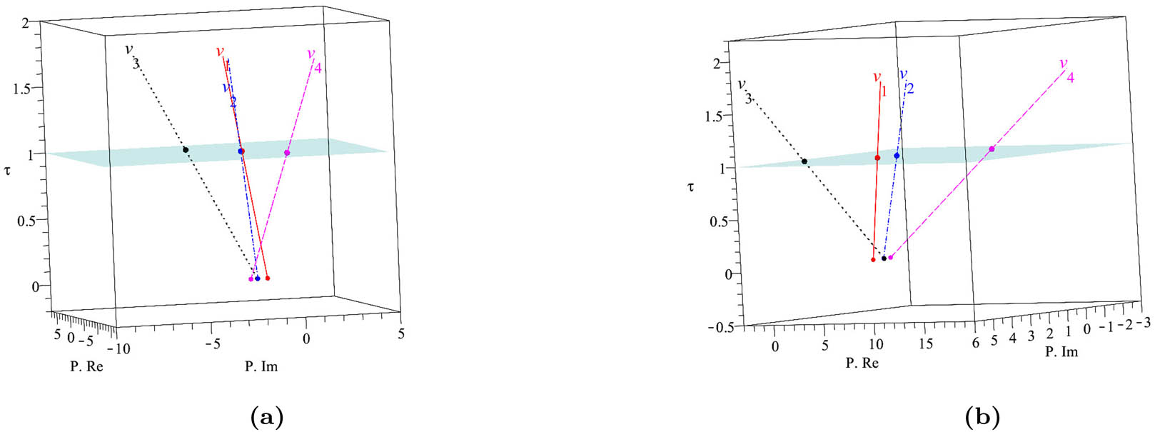
Hyperspheric homotopic tracking with
4.5 Case study 5
In [113], an electric circuit with a loop containing nonlinear elements was solved. In this case study, we will find the mesh currents for the electric circuit in Figure 16.
Electrical circuit with three meshes for case study 5.
The formulas for nonlinear impedances [113,114] are given by
where
For the mesh analysis of this problem, with nonlinear impedances in this case study, the following values are considered:
To determine the operating points of the nonlinear circuit, two different SPs were proposed:
Homotopic tracking for case study 5
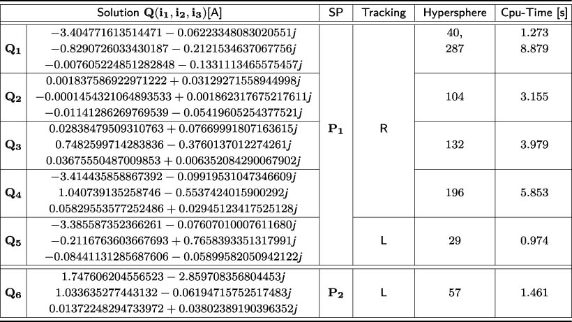 |
Figure 17 displays the homotopic tracking for the SP
Hyperspheric homotopic tracking with
Figure 18 presents the homotopic tracking on the left with SP
Hyperspheric homotopic tracking with
5 Numerical simulation and discussion
The computer utilized for the development of this work was equipped with an Intel Core i7-7700U CPU @ 3.60 GHz with 4 cores and 8 threads, an NVIDIA Corporation GP107 [GeForce GTX 1050 Ti] graphics card, and 64 GB of RAM, operating on Linux Ubuntu version 20.04.6 LTS. For the implementation of the homotopy algorithm with hyperspherical tracking, Maple 2019 software was employed. In addition, in the simulations, the built-in Maple command, fsolve, was used to validate the results.
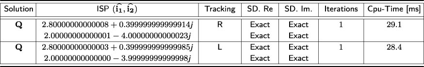
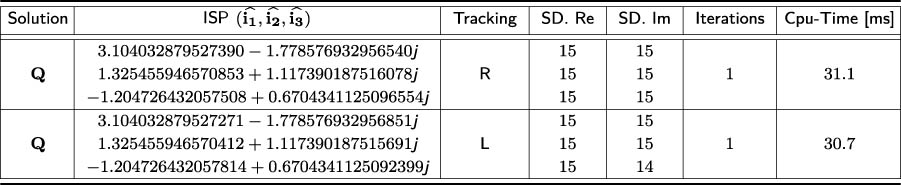
The analysis in this article focuses on identifying the complex roots of systems of algebraic equations, exploring the SDs found in the real and imaginary parts of each solution, as well as the iterations used. Tables 6, 7, 8, 9, 10 present the analysis of the SDs for the solutions of the case studies discussed in this article, utilizing the SPs provided by the linear interpolation of the homotopy algorithm. The criterion was to achieve more than ten SDs of accuracy in the solutions for the case studies. To validate the SD analysis, the SPs obtained from the interpolation (ISPs) were used in Maple’s fsolve function with the respective system of equations for all case studies to obtain the exact solution with 15 SDs.
Significant digits in the solutions for case study 1
 |
Significant digits in the solutions for case study 2
 |
Significant digits in the solutions for case study 3
 |
Significant digits in the solutions for case study 4
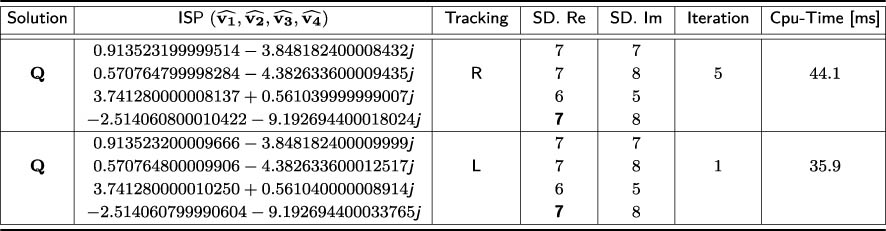 |
The bold values are the interpolated values for each variable, as defined in equation (19).
Significant digits in the solutions for case study 5
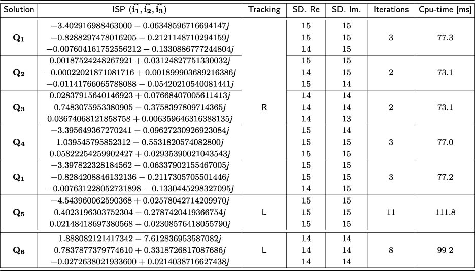 |
For case study 1, the real parts of all the solutions had 15 digits of accuracy. For
For case study 2, the analysis of SD was precise. The algebraically obtained solutions for case study 2 are
For case study 3, Table 8 shows high accuracy in the SD of all the electric currents obtained in the first refinement iteration for the electric circuit depicted in Figure 11. Only 14 SDs were achieved in the imaginary part of
For case study 4, the SDs obtained in the nodal voltages
Table 10 likewise demonstrates high accuracy in the SDs of the operating points for the electric circuit in case study 5. There is at least 14 SD in the real parts of the solutions, while the imaginary parts achieve 13 SD, as seen with
It is possible to determine the relative errors of all solutions presented in Tables 6–10 by employing the formula that associates the relative error with SDs [115,116], given by
where SD is the SDs,
Continuation homotopy with hyperspherical tracking can also experience numerical errors, similar to any numerical algorithm, such as round-off errors due to the finite precision of floating-point arithmetic in computers, numerical errors caused by nearly identical equations, convergence failure in N-R, or numerical instabilities [106,107]. These errors can cause the algorithm to lose homotopy path tracking. Furthermore, a study on the sensitivity of the algorithm indicates that it is generally more sensitive to the complexity of
CPU time for case
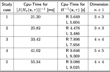 |
Table 12 presents a comparison of the computation times using differential path tracking and hyperspherical path tracking [34,39] for all the case studies analyzed in this work. The computation times obtained with hyperspherical path tracking are consistently shorter compared to those obtained with differential path tracking across all case studies. In addition, the number of iterations required in this study is lower when using hyperspherical path tracking compared to differential path tracking. It is noteworthy that in all case studies, all solutions were successfully found using hyperspherical path tracking, while differential path tracking only managed to identify some of them.
Comparison for solutions using hyperspherical path tracking vs differential path tracking
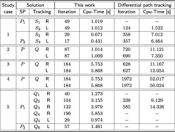 |
Furthermore, it is important to note that the inclusion of complex numbers in hyperspherical tracking significantly increases computation times, in contrast to those reported in the literature when real numbers are employed.
Table 13 presents a comparison of solutions obtained using homotopy with hyperspherical path tracking and the Super Ostrowski homotopy continuation method (SOHCM) [118,119]. The table displays the solutions found with Super-Ostrowski HCM in the path tracking, except in case study 4. In general, the CPU times with SOHCM are shorter than this work. However, in some cases, the SP leads to finding a different root. For instance, in this work, solution
Comparison for solutions using hyperspherical path tracking vs. super-Ostrowski HCM
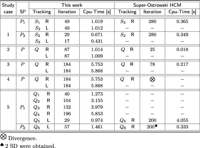 |
For case study 5, using SOHCM,
Likewise, the computational time increases as the complexity of the equation systems grows. Case study 5 requires a computational time of 4.005 [s] due to the system being nonlinear. In contrast, case study 4 does not have a solution. Furthermore, in [118], the structure of the homotopy includes a squared homotopic parameter, and the path tracking does not use any predictor, such as Euler, among others. However, it is possible to obtain
The path tracking behavior in Figures 10, 12, and 15 for case studies 2, 3 and 5, respectively, exhibits a linear trend because the systems of equations in theses case studies are linear. In contrast, Figures 7 and 8 in case study 1 and Figures 17 and 18 in case study 5 display nonlinear behavior. As the nonlinearity in the system of equations increases, the homotopic tracking demonstrates a more pronounced nonlinear behavior, as seen in Figure 17. However, Figures 19 and 20 show the graph homotopic parameter
Homotopic advance

Homotopic advance
For SP
Figure 21 shows the attractor basins for case study 1. Both figures were generated using the computer program Maple 21, with

Basins of attractions for case study 1. (a) Newton basin and (b) homotopy basin.
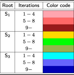
In the generated images, each point in the complex region that converges to a specific root is colored to match that root, with darker shades indicating a higher number of iterations and lighter shades fewer iterations. Points that do not converge within the iteration limit are colored gray. Figure 21 (a) shows the basins for a system with roots
In the figure, stability occurs when the initial point is located within a basin of attraction that contains a root. Conversely, instability arises when the SP leads to a trajectory that exits the colored zone and diverges to a distant region, potentially converging to a different root. Moreover, the basin boundaries generated by the N-R method intersect, forming the Julia set, a complex boundary where chaotic behavior manifests. It is important to keep in mind that a complex analytical function divides the plane into two distinct regions: the Fatou set, a stable area characterized by relatively simple dynamics, and the Julia set [14,120–122], which forms the chaotic boundary of the Fatou set [120,122].
Figure 21 (b) displays the attraction basins for the homotopy method with hyperspherical path tracking for
6 Conclusions
This study introduced a comprehensive exploration of the HCM combined with hyperspherical tracking to identify complex roots in systems of equations with applications to electrical circuits. The research conducted spanned a variety of case studies, ranging from systems of algebraic equations to complex electrical circuits with nonlinear elements. The findings of this study emphasize the efficacy and precision of the HCM with hyperspherical tracking in solving complex systems of equations.
The case studies presented illustrate the method’s capability to accurately determine complex roots, even in scenarios involving nonlinear elements and imaginary coefficients. The precision of the solutions was validated against existing literature and through the use of Maple’s fsolve function, demonstrating the method’s reliability and effectiveness. The analysis of SDs further underscored the method’s high level of accuracy, with most solutions achieving close to or exactly the desired number of SDs.
In addition, the study of basins obtained through homotopy requires an in-depth analysis of their behavior, as well as an examination of the potential existence of Julia sets or other related structures. The basin of attraction obtained through continuation homotopy extends the analysis of these basins while also broadening the study of continuation methods using this technique. On the other hand, it remains to study the causes of divergence of the homotopy in the basin of attraction.
Notably, the study also highlighted the method’s versatility in handling both linear and nonlinear systems, as well as its ability to find multiple operating points in electrical circuits. This versatility makes the HCM with hyperspherical tracking a valuable tool for researchers and practitioners in various fields, including electrical engineering, where complex systems of equations frequently arise.
Furthermore, the research presented contributes to the ongoing development of numerical methods for solving systems of equations. By demonstrating the practical applications of the HCM with hyperspherical tracking, this study adds to the body of knowledge and provides a foundation for future research in this area. The study proposes several avenues for future exploration. First, the homotopy routine with hyperspherical path tracking will be implemented in the
In conclusion, the HCM with hyperspherical tracking has proven to be a robust and precise approach for identifying complex roots in systems of equations. Its successful application to a diverse range of case studies underscores its potential as a numerical tool for solving complex problems in science and engineering. Future research could explore the method’s applicability to other complex systems and further optimize its implementation for enhanced efficiency and accuracy.
Acknowledgements
The first author is currently research fellow at Tecnológico Nacional de México en Celaya. He expresses his gratitude for the support received.
-
Funding information: This research did not receive any specific grant from funding agencies in the public, commercial, or not-for-profit sectors.
-
Author contributions: MASH, HJI, HVL: conceived and designed the experiments; performed the experiments; Analyzed and interpreted the data; contributed reagents, materials, analysis tools or data; wrote the article. MLQV, MLLG: performed the experiments; analyzed and interpreted the data; contributed reagents, materials, analysis tools, or data.
-
Conflict of interest: Dr. Hector Vazquez-Leal is an Editor of the Open Mathematics journal and was not involved in the review and decision-making process of this article.
-
Data availability statement: All data analyzed during this study are included in this published article.
References
[1] F. Rivero-Mendoza, Una introducción a los números complejos, Editorial Universidad de los Andes, Mérida, Venezuela, 2001.Search in Google Scholar
[2] H. Cardano, Artis magnae, sive de regulis algebraicis, liber unus, Franco Angeli, Milan, Italy, 2011. Search in Google Scholar
[3] C. R. Maluendas, Una breve historia imaginaria, Univ. Nac. Colomb. 1 (2019), no. 2, 1–9. https://editorial.konradlorenz.edu.co/2019/02/paskin-matematico.html. Search in Google Scholar
[4] R. Bombelli, LaAlgebra, Feltrinelli, Milan, Italy, 1966. Search in Google Scholar
[5] R. Descartes, La Géométrie, A. Herman, Librairie Scientifique, París, 1637. Search in Google Scholar
[6] B. Branner, Caspar Wessel. On the Analytical Representation of Direction: An Attempt Applied Chiefly to Solving Plane and Spherical Polygons, The Royal Danish Academy of Sciences and Letters, Copenhagen, Denmark, 1999. Search in Google Scholar
[7] J. R. Argand, Essai sur une manière de représenter les quantités imaginaires dans, les constructions géométriques, Gauthier-Villars, Imprimeur-Libraire, Paris, France, 1874. Search in Google Scholar
[8] L. Euleri, Introductio in analysin infinitorum, Tomus primus, Lausannae: apud Marcum-Michaelem Bousquet & Socies, Lausanne, Switzerland, 1748, http://hdl.handle.net/10481/31374.Search in Google Scholar
[9] L. Euler, Elements of Algebra, Springer-Verlag, WI, USA, 1972. Search in Google Scholar
[10] M. Hazewinkel, Encyclopaedia of Mathematics, Springer Science & Business Media, New York, USA, 1994. 10.1007/978-94-009-5983-5Search in Google Scholar
[11] S. Gutiérrez, Hamilton: La liberación del álgebra, Suma 49 (2005), no. 49, 95–99. https://revistasuma.fespm.es/sites/revistasuma.fespm.es/IMG/pdf/49/095-099.pdf. Search in Google Scholar
[12] J. M. Sánchez, Historias de Matemáticas: Hamilton y el descubrimiento de los cuaterniones, Pens. Mat. 1 (2011), no. 27. https://dialnet.unirioja.es/servlet/articulo?codigo=3744306. Search in Google Scholar
[13] C. P. Steinmetz, Complex Quatities and their use in electrical engineering, Proc. Int. Electr. Congr. Am. Inst. Electr. Eng. August 21st to 25th American Institute of Electrical Engineers, USA, 1893, pp. 33–75. Search in Google Scholar
[14] A. D. Wunsch, Variable Compleja con Aplicaciones, Pearson Educación, México, 1997. Search in Google Scholar
[15] J. A. Edminister, Circuitos Eléctricos, Serie Schaum, McGraw-Hill, México, 1982. Search in Google Scholar
[16] B. Mandelbrot, The Fractal Geometry of Nature, Free-man and Co., Mexico, 1977. Search in Google Scholar
[17] C. Monroy-Olivares, Curvas Fractales, Alfaomega, México, 2002. Search in Google Scholar
[18] M. J. Neve, Reinterpreting the Smith chart using conformal geometric algebra, IEEE Access 11 (2023), 138827–138838, DOI: https://doi.org/10.1109/ACCESS.2023.3340143. 10.1109/ACCESS.2023.3340143Search in Google Scholar
[19] A. N. Kani, Digital Signal Processing, CBS Publishers and Distributors, New Delhi, India, 2022. Search in Google Scholar
[20] G. A. Muñoz-Fernández and J. B. Seaone-Sepulveda, Fundamentos y Problemas Resueltos de Teoría Cualitativa de Ecuaciones Diferenciales, Ediciones Paraninfo, 2017. Search in Google Scholar
[21] A. L. Granados, Fractal techniques to measure the numerical instability of optimization methods, Comput. Mech. 15 (1995), no. 9, 369–374. Search in Google Scholar
[22] J. M. Gutiérrez, L. J. Hernández-Paricio, M. Marañón-Grandes, and M. T. Rivas-Rodríguez, Influence of the multiplicity of the roots on the basins of attraction of Newton’s method, Numer. Algorithms 66 (2014), 431–455. 10.1007/s11075-013-9742-7Search in Google Scholar
[23] J. M. Gutiérrez, Numerical properties of different root-finding algorithms obtained for approximating continuous Newton’s method, Algorithms 8 (2015), no. 4, 1210–1218, DOI: https://doi.org/10.3390/a8041210. 10.3390/a8041210Search in Google Scholar
[24] L. J. Hernández-Paricio, Bivariate Newton-Raphson method and toroidal attraction basins, Numer. Algorithms 71 (2016), 349–381, DOI: https://doi.org/10.1007/s11075-015-9996-3. 10.1007/s11075-015-9996-3Search in Google Scholar
[25] M. Sandoval-Hernandez, H. Vazquez-Leal, L. Hernandez-Martinez, U. A. Filobello-Nino, V. M. Jimenez-Fernandez, A. L. Herrera-May, et al., Approximation of Fresnel integrals with applications to diffraction problems, Math. Probl. Eng. 2018 (2018), 4031793, DOI: https://doi.org/10.1155/2018/4031793. 10.1155/2018/4031793Search in Google Scholar
[26] M. Maggiore, A Modern Introduction to Classical Electrodynamics, Oxford University Press, Oxford, UK, 2023. 10.1093/oso/9780192867421.001.0001Search in Google Scholar
[27] A. Cardama-Aznar, L. Jofre-Roca, J. M. Rius-Casals, J. Romeu-Robert, S. Blanch-Boris, and M. Ferrando-Bataller, Antenas, Univ. Politècnica de Catalunya, Alfaomega, Espannna, 2004. Search in Google Scholar
[28] J. J. Grainger and W. D. Stevenson Jr, Power System Analysis, McGraw-Hill Series in Electrical and Computer Engineering, Singapore, 1994. Search in Google Scholar
[29] K. Ogata, Ingeniería de Control Moderna, Quinta edición, Pearson Educación, México, 2010. Search in Google Scholar
[30] T. Deliyannis, Y. Sun, and J. K. Fidler, Continuous-time Active Filter Design, CRC Press, Boca Raton, Florida, USA, 2020. 10.1201/9781439821879Search in Google Scholar
[31] L. P. Huelsman, Active and Passive Analog Filter Design: An Introduction, McGraw Hill, New York, 1993. Search in Google Scholar
[32] J. V. Uspensky, Teoría de Ecuaciones, Limusa, México, 1987. Search in Google Scholar
[33] M. A. Jenkins and J. F. Traub, Algorithm 419: zeros of a complex polynomial [C2], Commun. ACM, 15 (1972), no. 2, 97–99, DOI: https://doi.org/10.1145/361254.361262. 10.1145/361254.361262Search in Google Scholar
[34] M. A. Sandoval-Hernandez, O. Alvarez-Gasca, A. D. Contreras-Hernandez, J. E. Pretelin-Canela, B. E. Palma-Grayeb, V. M. Jimenez-Fernandez, et al., Exploring the classic perturbation method for obtaining single and multiple solutions of nonlinear algebraic problems with application to microelectronic circuits, Int. J. Eng. Res. Technol. 8 (2019), no. 9, 636–645. https://www.ijert.org/exploring-the-classic-perturbation-method-for-obtaining-single-and-multiple-solutions-of-nonlinear-algebraic-problems-with-application-to-microelectronic-circuits. Search in Google Scholar
[35] F. Dubeau and C. Gnang, Fixed point and Newton’s methods in the complex plane, J. Complex Anal. 2018 (2018), 1–11, DOI: https://doi.org/10.1155/2018/7289092. 10.1155/2018/7289092Search in Google Scholar
[36] F. Çilingir, Singular perturbations arising in complex Newton’s method, Hacet. J. Math. Stat. 52 (2023), no. 5, 1–7, DOI: https://doi.org/10.15672/hujms.1132257. 10.15672/hujms.1132257Search in Google Scholar
[37] M. Sandoval-Hernandez, H. Vazquez-Leal, U. Filobello-Nino, E. De-Leo-Baquero, A. C. Bielma-Perez, J. C. Vichi-Mendoza, et al., The quadratic equation and its numerical roots, Int. J. Eng. Res. Technol. 10 (2021), no. 6, 301–305. https://www.ijert.org/research/the-quadratic-equation-and-its-numerical-roots-IJERTV10IS060100.pdf. Search in Google Scholar
[38] K. Gdawiec, I. K. Argyros, S. Qureshi, and A. Soomro, An optimal homotopy continuation method: Convergence and visual analysis, J. Comput. Sci. 74 (2023), 1–12, DOI: https://doi.org/10.1016/j.jocs.2023.102166. 10.1016/j.jocs.2023.102166Search in Google Scholar
[39] T. L. Wayburn and J. D. Seader, Homotopy continuation methods for computer-aided process design, Comput. Chem. Eng. 11 (1987), no. 1, 7–25, DOI: https://doi.org/10.1016/0098-1354(87)80002-9. 10.1016/0098-1354(87)80002-9Search in Google Scholar
[40] J. Farhang, J. D. Seader, and S. Khaleghi, Global solution approaches in equilibrium and stability analysis using homotopy continuation in the complex domain, Comput. Chem. Eng. 32 (2008), no. 10, 2333–2345, DOI: https://doi.org/10.1016/j.compchemeng.2007.12.001. 10.1016/j.compchemeng.2007.12.001Search in Google Scholar
[41] H. Vazquez-Leal, et al., Biparameter homotopy-based direct current simulation of multistable circuits, Br. J. Math. Comput. Sci. 2 (2012), no. 3, 137–150, https://journaljamcs.com/index.php/JAMCS/article/view/1240.10.9734/BJMCS/2012/1346Search in Google Scholar
[42] M. D. L. L. López-González, M. L. Quemada-Villagómez, M. G. Martínez-González, J. M. Oliveros-Muñoz, and H. Jiménez-Islas, A novel predictive homotopic path tracking algorithm to solve non-linear algebraic equations, Can. J. Chem. Eng. 101 (2023), no. 6, 3382–3408, DOI: https://doi.org/10.1002/cjce.24694. 10.1002/cjce.24694Search in Google Scholar
[43] J. R. White, Case study: Protein folding using homotopy methods, Scientific Computing with Case Studies, SIAM Press, Philadelphia, USA, 2009, pp. 1–8. https://www.cs.umd.edu/oleary/SCCS/supp/White/Homotopy_paper.pdf. Search in Google Scholar
[44] H. Jimenez-Islas, Sehpe: Programa para la solución de sistemas de ecuaciones no lineales mediante método homotópico con seguimiento hiperesférico, Av. Ing. Quím. 6 (1996), no. 2, 174–179. Search in Google Scholar
[45] J. M. Oliveros-Munoz and H. Jiménez-Islas, Hyperspherical path tracking methodology as correction step in homotopic continuation methods, Chem. Eng. Sci. 97 (2013), no. 28, 413–429, DOI: https://doi.org/10.1016/j.ces.2013.03.053. 10.1016/j.ces.2013.03.053Search in Google Scholar
[46] H. Jiménez-Islas, M. Calderón-Ramírez, G. M. Martínez-González, M. P. Calderón-Álvarado, and J. M. Oliveros-Munoz, Multiple solutions for steady differential equations via hyperspherical path-tracking of homotopy curves, Comput. Math. Appl. 78 (2020), no. 8, 2216–2239, DOI: https://doi.org/10.1016/j.camwa.2019.10.023. 10.1016/j.camwa.2019.10.023Search in Google Scholar
[47] L. O. Chua, Nonlinear Network Analysis-the Parametric Approach, Ph.D. Thesis, University of Illinois, June 1964. https://hdl.handle.net/2142/74281. Search in Google Scholar
[48] L. O., Chua and A. Ushida, A switching-parameter algorithm for finding multiple solutions of nonlinear resistive networks, Int. J. Circuit Theory Appl. 4 (1976), no. 3, 215–237, DOI: https://doi.org/10.1002/cta.4490040302. 10.1002/cta.4490040302Search in Google Scholar
[49] L. O. Chua and N. N. Wang, A new approach to overcome the overflow problem in computer-aided analysis of nonlinear resistive circuits, Int. J. Circuit Theory Appl. 3 (1975), no. 3, 261–284, DOI: https://doi.org/10.1002/cta.4490030305. 10.1002/cta.4490030305Search in Google Scholar
[50] L. Trajkovic, R. C. Melville, and S.-C. Fang, Finding DC operating points of transistor circuits using homotopy methods, 1991 IEEE Int. Symp. Circuits Syst. Singapore 2 (1991), 758–761, DOI: https://doi.org/10.1109/ISCAS.1991.176473. 10.1109/ISCAS.1991.176473Search in Google Scholar
[51] M. Tolikas, L. Trajkovic, and M. D. Ilic, Homotopy methods for solving decoupled power flow equations, 1992 IEEE Int. Symp. Circuits Syst. San Diego, CA, USA 6 (1992), 2833–2839, DOI: https://doi.org/10.1109/ISCAS.1992.230609. 10.1109/ISCAS.1992.230609Search in Google Scholar
[52] R. C. Melville, L. Trajkovic, S. -C. Fang, and L. T. Watson, Artificial parameter homotopy methods for the DC operating point problem, IEEE Trans. Comput.-Aided Des. Integr. Circuits Syst. 12 (1993), no. 6, 861–877, DOI: https://doi.org/10.1109/43.229761. 10.1109/43.229761Search in Google Scholar
[53] A. Dyes, E. Chan, H. Hofmann, W. Horia, and L. Trajkovic, Simple implementations of homotopy algorithms for finding DC solutions of nonlinear circuits, 1999 IEEE Int. Symp. Circuits Syst. Orlando, FL, USA 6 (1999), 290–293, DOI: https://doi.org/10.1109/ISCAS.1999.780152. 10.1109/ISCAS.1999.780152Search in Google Scholar
[54] L. Trajkovic, Homotopy Methods for Computing DC Operating Points, Wiley, 1999. 10.1002/047134608X.W2526Search in Google Scholar
[55] L. Kronenberg, W. Mathis, and L. Trajkovic, Limitations of criteria for testing transistor circuits for multiple DC operating points, Proc. 43rd IEEE Midwest Symp. Circuits Syst. Lansing, MI, USA 1 (2000), 148–151, DOI: https://doi.org/10.1109/MWSCAS.2000.951607. 10.1109/MWSCAS.2000.951607Search in Google Scholar
[56] L. Trajkovic, Homotopy Algorithms for Finding DC and Steady-State Solutions of Nonlinear Circuits, Electronics and Signal Processing Summer Symposium-LEOS, British Columbia, Canada, 2002. Search in Google Scholar
[57] L. Trajkovic, R. C. Melville, and S.-C. Fang, Improving DC convergence in a circuit simulator using a homotopy method, Proc. IEEE 1991 Custom Integr. Circuits Conf. San Diego, CA, USA, 1991, pp. 8.1/1–8.1/4, DOI: https://doi.org/10.1109/CICC.1991.164032. 10.1109/CICC.1991.164032Search in Google Scholar
[58] L. Trajkovic, E. Fung, and S. Sanders, HomSPICE: simulator with homotopy algorithms for finding DC and steady-state solutions of nonlinear circuits, 1998 IEEE Int. Symp. Circuits Syst. Monterey, CA, USA 6 (1998), 227–231, DOI: https://doi.org/10.1109/ISCAS.1998.705253. 10.1109/ISCAS.1998.705253Search in Google Scholar
[59] H. Vazquez-Leal, A. Marin-Hernandez, Y. Khan, A. Yıldırım, U. Filobello-Nino, R. Castaneda-Sheissa, et al., Exploring collision-free path planning by using homotopy continuation methods, Appl. Math. Comput. 219 (2013), no. 14, 7514–7532, DOI: https://doi.org/10.1016/j.amc.2013.01.038. Search in Google Scholar
[60] G. Diaz-Arango, H. Vazquez-Leal, L. Hernandez-Martinez, M. T. Sanz-Pascual, and M. Sandoval-Hernandez, Homotopy path planning for terrestrial robots using spherical algorithm, IEEE Trans. Autom. Sci. Eng. 15 (2017), no. 2, 567–585, DOI: https://doi.org/10.1109/TASE.2016.2638208. 10.1109/TASE.2016.2638208Search in Google Scholar
[61] G. C. Velez-Lopez, H. Vazquez-Leal, L. Hernandez-Martinez, A. Sarmiento-Reyes, G. Diaz-Arango, and J. Huerta-Chua, et al., A novel collision-free homotopy path planning for planar robotic arms, Sensors 22 (2022), no. 11:4022, 1–27, DOI: https://doi.org/10.3390/s22114022. 10.3390/s22114022Search in Google Scholar PubMed PubMed Central
[62] G. C. Velez-Lopez, L. Hernandez-Martinez, H. Vazquez-Leal, M. A. Sandoval-Hernández, V. M. Jimenez-Fernandez, and M. Gonzalez-Lee, Collision-free path planning applied to multi-degree-of-freedom robotic arms using homotopy methods, IEEE Access 12 (2024), 150702–150718, DOI: https://doi.org/10.1109/ACCESS.2024.3479095. 10.1109/ACCESS.2024.3479095Search in Google Scholar
[63] M. L. Quemada-Villagómez, M. D. L. L. López-González, J. M. Oliveros-Muñoz, and H. Jiménez-Islas, Ensennnanza del método de continuación homotópica con seguimiento hiperesférico para estudiantes de ingeniería, Acta Univ. 32 (2022), 1–43, DOI: https://doi.org/10.15174/au.2022.3358. 10.15174/au.2022.3358Search in Google Scholar
[64] M. A. Sandoval-Hernández, H Vázquez-Leal, J. Huerta-Chua, U. A. Filobello-Nino, and D. Mayorga-Cruz, La didáctica del cálculo integral: el caso de los procedimientos de integración, Rev. Iberoam. Investig. Desarro. Educ. 13 (2022), no. 25, 1–28, DOI: https://doi.org/10.23913/ride.v13i25.1245. 10.23913/ride.v13i25.1245Search in Google Scholar
[65] R. C. Uriza, G. M. Espinosa, and D. R. Gasperini, Análisis del discurso matemático escolar en los libros de texto: una mirada desde la teoría socioepistemológica, Av. Investig. Educ. Mat. 8 (2015), 9–28, DOI: https://doi.org/10.35763/aiem.v1i8.123. 10.35763/aiem.v1i8.123Search in Google Scholar
[66] C. Prieto-De-Castro, Biografía Henri Poincaré, Instituto de Matemáticas, Universidad Nacional Autónoma de México, 1977.Search in Google Scholar
[67] W. S. Massey, Introdución a la Topología Algebraica, Reverté, España, 2006. Search in Google Scholar
[68] M. Macho-Stadler, Homotopía, Publicaciones de divulgación, Universidad del País Vasco-Euskal Herriko Unibertsitatea, 2003. Search in Google Scholar
[69] J. Strom, Modern Classical Homotopy Theory, Graduate Studies in Mathematics, Vol. 127, American Mathematical Society, 2011. 10.1090/gsm/127Search in Google Scholar
[70] S. Lipschutz, Theory and Problems of General Topology, Schaumas Outline Series, Mc Graw-Hill, 1965. Search in Google Scholar
[71] M. Macho-Stadler, Qué es la Topología?, Publicaciones de divulgación, Universidad del País Vasco-Euskal, Herriko Unibertsitatea, Euskadi, 2018, https://divulgacioncientificadecientificos.blogspot.com/2018/08/que-es-la-topologia-marta-macho-stadler.html. Search in Google Scholar
[72] L. E. J. Brouwer, Beweis des Jordanschen Kurvensatzes, Math. Ann. 69 (1910), 169–175, DOI: https://doi.org/10.1007/BF01456867. 10.1007/BF01456867Search in Google Scholar
[73] L. E. J. Brouwer, Über Abbildung von Mannigfaltigkeiten, Math. Ann. Springer 71 (1911), 97–115, DOI: https://doi.org/10.1007/BF01456931. 10.1007/BF01456931Search in Google Scholar
[74] C. B. García and W. I. Zangwill, Pathways to Solution Fixed Point in Equilibria, Prentice Hall, 1981. Search in Google Scholar
[75] J. Leray and J. Schauder, Topologie et équations fonctionnelles, Ann. Sci. Éc. Norm. Supér. 51 (1934), 45–78. http://www.numdam.org/item/10.24033/asens.836.pdf. 10.24033/asens.836Search in Google Scholar
[76] F. A. Ficken, The continuation method for functional equations, Comm. Pure Appl. Math. 4 (1951), no. 4, 435–456, DOI: https://doi.org/10.1002/cpa.3160040405. 10.1002/cpa.3160040405Search in Google Scholar
[77] C. B. Haselgrove, The solution of non-linear equations and of differential equations with two-point boundary conditions, Computer J. Oxford University Press 4 (1961), no. 3, 255–259, DOI: https://doi.org/10.1093/comjnl/4.3.255. 10.1093/comjnl/4.3.255Search in Google Scholar
[78] D. F. Davidenko, On the approximate solution of a system of nonlinear equations, Ukr. Mat. Zh. 5 (1953), no. 2, 196–206. Search in Google Scholar
[79] E. Lahaye, Use Methode de Resolution daune Categorie deeeeeéquations Transcendentes, C.R. Acad. Sci. Paris 198 (1934), 1840–1842. Search in Google Scholar
[80] D. F. Davidenko, On the new method of numerically integrating a system of nonlinear equations, Dokl. Akad. Nauk SSSR 88 (1953), 601–604. Search in Google Scholar
[81] W. C., Rheinboldt, An adaptive continuation process for solving systems of nonlinear equations, Univ. Md. Banach Cent. Publ. 3 (1978), no. 1, 129–142. http://eudml.org/doc/208686. 10.4064/-3-1-129-142Search in Google Scholar
[82] P. Deuflhard, A Step Size Control for Continuation Methods and its Special Application to Multiple Shooting Techniques, Univertitat Hidelberg, Instiut für Angewandte Mathematik, Numerische Mathematik, Springer-Verlag, 1979. 10.1007/BF01399549Search in Google Scholar
[83] J. N. Lyness and B. J. J. McHugh, Integration over multidimensional hypercubes I. A progressive procedure, Comput. J. 6 (1963), no. 3, 264–270, DOI: https://doi.org/10.1093/comjnl/6.3.264. 10.1093/comjnl/6.3.264Search in Google Scholar
[84] E. L. Allgower and K. Georg, Introduction to numerical continuation methods, Classics in Applied Mathematics, Springer-Verlag, Philadelphia, 2003. 10.1137/1.9780898719154Search in Google Scholar
[85] H. Jiménez-Islas, Paquete Computacional Para la Solución de Sistemas de Ecuaciones no Lineales, PhD thesis, Instituto Tecnológico de Celaya, 1988, DOI: https://doi.org/10.13140/RG.2.2.12052.31363, https://acortar.link/cPGvWn. Search in Google Scholar
[86] A. Ushida and L. O. Chua, Tracing solution curves of non-linear equations with sharp turning points, Int. J. Circuit Theory Appl. 12 (1984), no. 1, 1–21, DOI: https://doi.org/10.1002/cta.4490120102. 10.1002/cta.4490120102Search in Google Scholar
[87] Y. Shinohara, A geometric method of numerical solution of nonlinear equation and error estimation by Urabeas proposition, RIMS Kyoto Univ. 5 (1969), no. 1, 1–9, DOI: https://doi.org/10.2977/PRIMS/1195194748. 10.2977/prims/1195194748Search in Google Scholar
[88] R. K. Brayton, F. G. Gustavson, and G. D. Hachtel, A new efficient algorithm for solving differential-algebraic systems using implicit backward differentiation formulas, Proc. IEEE 60 (1972), no. 1, 98–108, DOI: https://doi.org/10.1109/PROC.1972.8562. 10.1109/PROC.1972.8562Search in Google Scholar
[89] C. W. Gear, The automatic integration of ordinary differential equations, Commun. ACM 14 (1971), no. 3, 176–179, DOI: https://doi.org/10.1145/362566.362571. 10.1145/362566.362571Search in Google Scholar
[90] K. Yamamura, Simple algorithms for tracing solution curves, IEEE Trans. Circuits Syst. I Fundam. Theory Appl. 40 (1993), no. 8, 537–541, DOI: https://doi.org/10.1109/81.242328. 10.1109/81.242328Search in Google Scholar
[91] R. W. Klopfenstein, Zeros of nonlinear functions, RCA Lab. N.J. ACM Digit. Libr. 8 (1961), no. 3, 366–373, DOI: https://doi.org/10.1145/321075.321080. 10.1145/321075.321080Search in Google Scholar
[92] E. Allgower and K. Georg, Introduction to Numerical Continuation Methods, Classics in Applied Mathematics, Springer-Verlag, Philadelphia, USA, 1990. 10.1007/978-3-642-61257-2Search in Google Scholar
[93] J. C. Alexander and J. A. Yorke, The homotopy continuation method: numerically implementable topological procedures, Trans. Amer. Math. Soc. 242 (1978), 271–284, DOI: https://doi.org/10.1090/S0002-9947-1978-0478138-5. 10.1090/S0002-9947-1978-0478138-5Search in Google Scholar
[94] S. N. Chow, J. Mallet-Paret, and J. A. Yorke, Finding zeros of maps: homotopy methods that are constructive with probability one, Math. Comput. 32 (1978), 887–899, DOI: https://doi.org/10.1090/S0025-5718-1978-0492046-9. 10.1090/S0025-5718-1978-0492046-9Search in Google Scholar
[95] L. T. Watson, Engineering applications of the Chow-Yorke algorithm, Appl. Math. Comput. 9 (1981), no. 2, 111–133, DOI: https://doi.org/10.1016/0096-3003(81)90010-2. 10.1016/0096-3003(81)90010-2Search in Google Scholar
[96] S. N. Chow, J. Mallet-Paret, and J. A. Yorke, A homotopy method for locating all zeros of a system of polynomials, Lecture Notes Math. 730 (1979). 77–88, DOI: https://doi.org/10.1007/BFb0064312. 10.1007/BFb0064312Search in Google Scholar
[97] T. Y. Li, T. Sauer, and J. A. Yorke, The Cheateras homotopy: an efficient procedure for solving systems of polynomial equations, SIAM J. Numer. Anal. 26 (1989), no. 5, 1241–1251, DOI: https://doi.org/10.1137/0726069. 10.1137/0726069Search in Google Scholar
[98] J. D. Seader, M. Kuno, W. Lin, S. A. Johnson, K. Unsworth, and J. W. Wiskin, Mapped continuation methods for computing all solutions to general systems of nonlinear equations, Comput. Chem. Eng. 14 (1990), no. 1, 71–85, DOI: https://doi.org/10.1016/0098-1354(90)87006-B. 10.1016/0098-1354(90)87006-BSearch in Google Scholar
[99] M. Kuno and J. D. Seader, Computing all real solutions systems of nonlinear equations with a global fixed-point homotopy, Ind. Eng. Chem. Res. 27 (1988), no. 7, 1320–1329, DOI: https://doi.org/10.1021/ie00079a037. 10.1021/ie00079a037Search in Google Scholar
[100] S. H. Choi and N. L. Book, Unreachable roots for global homotopy continuation methods, AIChE J. 37 (1991), no. 7, 1093–1095, DOI: https://doi.org/10.1002/aic.690370713. 10.1002/aic.690370713Search in Google Scholar
[101] S. Khaleghi-Rahimian, F. Jalali, J. D. Seader, and R. E. White, A new homotopy for seeking all real roots of a nonlinear equation, Comput. Chem. Eng. 35 (2011), no. 3 403–411, DOI: https://doi.org/10.1016/j.compchemeng.2010.04.007. 10.1016/j.compchemeng.2010.04.007Search in Google Scholar
[102] K. Yamamura, A fixed-point homotopy method for solving modified nodal equations, IEEE Trans. Circuits Syst. I Fundam. Theory Appl. 46 (1999), no. 6, 654–665, DOI: https://doi.org/10.1109/81.768822. 10.1109/81.768822Search in Google Scholar
[103] D. M. Wolf and S. R. Sanders, Multiparameter, homotopy methods for finding DC operating points of nonlinear circuits, IEEE Trans. Circuits Syst. I Fundam. Theory Appl. 43 (1996), no. 10, 824–838, DOI: https://doi.org/10.1109/81.538989. 10.1109/81.538989Search in Google Scholar
[104] M. Sosonkina, L. T. Watson, and D. E. Stewart, Note on the end game in homotopy zero curve tracking, ACM Trans. Math. Software 22 (1996), no. 3, 281–287, DOI: https://doi.org/10.1145/232826.232843. 10.1145/232826.232843Search in Google Scholar
[105] H. Vazquez-Leal, A. Marin-Hernandez, Y. Khan, A Yıldırım, U. Filobello-Nino, and R. Castaneda-Sheissa, et al., Exploring collision-free path planning by using homotopy continuation methods, Appl. Math. Comput. Elsevier 219 (2013), no. 14, 7514–7532, DOI: https://doi.org/10.1016/j.amc.2013.01.038. 10.1016/j.amc.2013.01.038Search in Google Scholar
[106] R. Burden and J. Faires, Numerical Analysis, 9th edn., Cengage Learning, Boston, 2011. Search in Google Scholar
[107] S. C. Chapra and R. P. Canale. Métodos Numéricos Para Ingenieros, McGraw-Hill, Mexico, 2011. Search in Google Scholar
[108] A. S. Sedra, K. C. Smith, T .C. Carusone, and V. Gaudet, Microelectronic Circuits, 8th edn., Oxford University Press, Oxford, 2020. Search in Google Scholar
[109] R. Boylestad and L. Nashelsky, Electrónica: teoría de circuitos y dispositivos electrónicos, Pearson Educación, Mexico, 2009. Search in Google Scholar
[110] R. L. Tokheim, Digital Electronics, Glencoe, Glencoe, UK, 1994. Search in Google Scholar
[111] J. M. Angulo-Usategui, B. Garcia-Zapirain, I. Angulo-Martínez, and J. V. Sáez, Microcontroladores avanzados dsPIC: controladores digitales de señales: arquitectura, programación y aplicaciones, Thomson, Mexico, 2006. Search in Google Scholar
[112] B. B. Brey, Los microprocesadores intel: arquitectura, programación e interfaces, Pearson-Prentice-Hall, Mexico, 2007. Search in Google Scholar
[113] J. S. Thomsen and S. Schlesinger, Analysis of nonlinear circuits using impedance concepts, IRE Trans. Circuit Theory 2 (1955), no. 3, 271–278, DOI: https://doi.org/10.1109/TCT.1955.1085250. 10.1109/TCT.1955.1085250Search in Google Scholar
[114] J. S. Thomsen, Graphical analysis of nonlinear circuits using impedance concepts, J. Appl. Phys. AIP Publishing 24 (1953), no. 11, 1379–1382, DOI: https://doi.org/10.1063/1.1721182. 10.1063/1.1721182Search in Google Scholar
[115] M. A. Sandoval-Hernández, H. Vazquez-Leal, U. A. Filobello-Nino, G. J. Morales-AlarcóN, G. C. Velez-LóPez, and R. CastañEda-Sheissa, et al., Using Horner’s algorithm to reduce computing times, Int. J. Eng. Res. Technol. 12 (2023), no. 06, 325–331. https://www.ijert.org/research/using-horners-algorithm-to-reduce-computing-times-IJERTV12IS060143.pdf. Search in Google Scholar
[116] H. Vazquez-Leal, M. A. Sandoval-Hernandez, J. L. Garcia-Gervacio, A. L. Herrera-May, and U. A. Filobello-Nino, PSEM aproximations for both branches of Lambert W with applications, Discrete Dyn. Nat. Soc. 2019 (2019), 267951, DOI: https://doi.org/10.1155/2019/8267951. 10.1155/2019/8267951Search in Google Scholar
[117] L. T. Watson, A globally convergent algorithm for computing fixed-points of C2 maps, Appl. Math. Comput. 5 (1979), no. 4, 297–311, DOI: https://doi.org/10.1016/0096-3003(79)90020-1. 10.1016/0096-3003(79)90020-1Search in Google Scholar
[118] H. Mohamad-Nor, A. Rahman, A. I. Md-Ismail, and A. Abdul-Majid, Super Ostrowski homotopy continuation method for solving polynomial system of equations, Matematika 32 (2016), no. 1, 53–67, DOI: https://doi.org/10.11113/matematika.v32.n1.685. 10.11113/matematika.v32.n1.685Search in Google Scholar
[119] H. Mohamad-Nor, A. I. Md-Ismail, and A. Abdul-Majid, Linear fixed-point function for solving system of polynomial equations, AIP Conf. Proc. 1602 (2014), no. 1, 105–112, DOI: https://doi.org/10.1063/1.4882474. 10.1063/1.4882474Search in Google Scholar
[120] S. Sutherland, An introduction to Julia and Fatou sets, in: Fractals, Wavelets, and their Applications: Contributions from the International Conference and Workshop on Fractals and Wavelets, vol. 92, Springer Proceedings in Mathematics & Statistics, Switzerland, 2014, pp. 37–60. 10.1007/978-3-319-08105-2_3Search in Google Scholar
[121] G. N. Rubiano, Método de Newton, Mathematica y fractales: historia de una página, Bol. Mat. 14 (2007), no. 1, 44–63.Search in Google Scholar
[122] K. Madhu and J. Jayaraman, Higher order methods for nonlinear equations and their basins of attraction, Mathematics 4 (2016), no. 2, 22, DOI: https://doi.org/10.3390/math4020022. 10.3390/math4020022Search in Google Scholar
[123] B. Haible and R. B. Kreckel, CLN, A Class Library for Numbers, GiNaC C++ library, Germany, 1996. https://www.ginac.de/CLN/cln.pdf. Search in Google Scholar
[124] P. R. Bell and J. M. Doughertym, Nonlinear image processing method, IEEE Trans. Nucl. Sci. 25 (1978), no. 2, 928–938, DOI: https://doi.org/10.1109/TNS.1978.4329438. 10.1109/TNS.1978.4329438Search in Google Scholar
[125] H. Daisuke, E. Takaya, M. Kadowaki, Y. Kobayashi, and T. Ueda, Effect of the pixel interpolation method for downsampling medical images on deep learning accuracy, J. Comput. Commun. 9 (2021), no. 11, 150–156, DOI: https://doi.org/10.4236/jcc.2021.911010. 10.4236/jcc.2021.911010Search in Google Scholar
[126] A. Singh and J. Singh, Review and comparative analysis of various image interpolation techniques, 2019 IEEE 2nd Int. Conf. Intell. Comput. Instrument. Control Technol. Kannur, India 1 (2019), 1214–1218, DOI: https://doi.org/10.1109/ICICICT46008.2019.8993258. 10.1109/ICICICT46008.2019.8993258Search in Google Scholar
© 2025 the author(s), published by De Gruyter
This work is licensed under the Creative Commons Attribution 4.0 International License.
Articles in the same Issue
- On I-convergence of nets of functions in fuzzy metric spaces
- Special Issue on Contemporary Developments in Graphs Defined on Algebraic Structures
- Forbidden subgraphs of TI-power graphs of finite groups
- Finite group with some c#-normal and S-quasinormally embedded subgroups
- Classifying cubic symmetric graphs of order 88p and 88p 2
- Two-sided zero-divisor graphs of orientation-preserving and order-decreasing transformation semigroups
- Simplicial complexes defined on groups
- Further results on permanents of Laplacian matrices of trees
- Algebra
- Classes of modules closed under projective covers
- On the dimension of the algebraic sum of subspaces
- Green's graphs of a semigroup
- On an uncertainty principle for small index subgroups of finite fields
- On a generalization of I-regularity
- Algorithm and linear convergence of the H-spectral radius of weakly irreducible quasi-positive tensors
- The hyperbolic CS decomposition of tensors based on the C-product
- On weakly classical 1-absorbing prime submodules
- Equational characterizations for some subclasses of domains
- Algebraic Geometry
- Spin(8, ℂ)-Higgs bundles fixed points through spectral data
- Embedding of lattices and K3-covers of an Enriques surface
- Kodaira-Spencer maps for elliptic orbispheres as isomorphisms of Frobenius algebras
- Applications in Computer and Information Sciences
- Dynamics of particulate emissions in the presence of autonomous vehicles
- Exploring homotopy with hyperspherical tracking to find complex roots with application to electrical circuits
- Category Theory
- The higher mapping cone axiom
- Combinatorics and Graph Theory
- 𝕮-inverse of graphs and mixed graphs
- On the spectral radius and energy of the degree distance matrix of a connected graph
- Some new bounds on resolvent energy of a graph
- Coloring the vertices of a graph with mutual-visibility property
- Ring graph induced by a ring endomorphism
- A note on the edge general position number of cactus graphs
- Complex Analysis
- Some results on value distribution concerning Hayman's alternative
- Freely quasiconformal and locally weakly quasisymmetric mappings in metric spaces
- A new result for entire functions and their shifts with two shared values
- On a subclass of multivalent functions defined by generalized multiplier transformation
- Singular direction of meromorphic functions with finite logarithmic order
- Growth theorems and coefficient bounds for g-starlike mappings of complex order λ
- Refinements of inequalities on extremal problems of polynomials
- Control Theory and Optimization
- Averaging method in optimal control problems for integro-differential equations
- On superstability of derivations in Banach algebras
- The robust isolated calmness of spectral norm regularized convex matrix optimization problems
- Observability on the classes of non-nilpotent solvable three-dimensional Lie groups
- Differential Equations
- The ill-posedness of the (non-)periodic traveling wave solution for the deformed continuous Heisenberg spin equation
- A note on the global existence and boundedness of an N-dimensional parabolic-elliptic predator-prey system with indirect pursuit-evasion interaction
- Blow-up of solutions for Euler-Bernoulli equation with nonlinear time delay
- Periodic or homoclinic orbit bifurcated from a heteroclinic loop for high-dimensional systems
- Regularity of weak solutions to the 3D stationary tropical climate model
- Local minimizers for the NLS equation with localized nonlinearity on noncompact metric graphs
- Global existence and blow-up of solutions to pseudo-parabolic equation for Baouendi-Grushin operator
- Bubbles clustered inside for almost-critical problems
- Existence and multiplicity of positive solutions for multiparameter periodic systems
- Existence of positive periodic solutions for evolution equations with delay in ordered Banach spaces
- On a nonlinear boundary value problems with impulse action
- Normalized ground-states for the Sobolev critical Kirchhoff equation with at least mass critical growth
- Multiple positive solutions to a p-Kirchhoff equation with logarithmic terms and concave terms
- Infinitely many solutions for a class of Kirchhoff-type equations
- Real and non-real eigenvalues of regular indefinite Sturm–Liouville problems
- Existence of global solutions to a semilinear thermoelastic system in three dimensions
- Limiting profile of positive solutions to heterogeneous elliptic BVPs with nonlinear flux decaying to negative infinity on a portion of the boundary
- Morse index of circular solutions for repulsive central force problems on surfaces
- Differential Geometry
- On tangent bundles of Walker four-manifolds
- Pedal and negative pedal surfaces of framed curves in the Euclidean 3-space
- Discrete Mathematics
- Eventually monotonic solutions of the generalized Fibonacci equations
- Dynamical Systems Ergodic Theory
- Dynamical properties of two-diffusion SIR epidemic model with Markovian switching
- A note on weighted measure-theoretic pressure
- Pullback attractors for a class of second-order delay evolution equations with dispersive and dissipative terms on unbounded domain
- Pullback attractor of the 2D non-autonomous magneto-micropolar fluid equations
- Functional Analysis
- Spectrum boundary domination of semiregularities in Banach algebras
- Approximate multi-Cauchy mappings on certain groupoids
- Investigating the modified UO-iteration process in Banach spaces by a digraph
- Tilings, sub-tilings, and spectral sets on p-adic space
- Continuity and essential norm of operators defined by infinite tridiagonal matrices in weighted Orlicz and l∞ spaces
-
A family of commuting contraction semigroups on
- q-Stirling sequence spaces associated with q-Bell numbers
- Chlodowsky variant of Bernstein-type operators on the domain
- Hyponormality on a weighted Bergman space of an annulus with a general harmonic symbol
- Characterization of derivations on strongly double triangle subspace lattice algebras by local actions
- Fixed point approaches to the stability of Jensen’s functional equation
- Geometry
- The regularity of solutions to the Lp Gauss image problem
- Solving the quartic by conics
- Group Theory
- On a question of permutation groups acting on the power set
- A characterization of the translational hull of a weakly type B semigroup with E-properties
- Harmonic Analysis
- Eigenfunctions on an infinite Schrödinger network
- Maximal function and generalized fractional integral operators on the weighted Orlicz-Lorentz-Morrey spaces
- Subharmonic functions and associated measures in ℝn
- Mathematical Logic, Model Theory and Foundation
- A topology related to implication and upsets on a bounded BCK-algebra
- Boundedness of fractional sublinear operators on weighted grand Herz-Morrey spaces with variable exponents
- Number Theory
- Fibonacci vector and matrix p-norms
- Recurrence for probabilistic extension of Dowling polynomials
- Carmichael numbers composed of Piatetski-Shapiro primes in Beatty sequences
- The number of rational points of some classes of algebraic varieties over finite fields
- Classification and irreducibility of a class of integer polynomials
- Decompositions of the extended Selberg class functions
- Joint approximation of analytic functions by the shifts of Hurwitz zeta-functions in short intervals
- Fibonacci Cartan and Lucas Cartan numbers
- Recurrence relations satisfied by some arithmetic groups
- The hybrid power mean involving the Kloosterman sums and Dedekind sums
- Numerical Methods
- A modified predictor–corrector scheme with graded mesh for numerical solutions of nonlinear Ψ-caputo fractional-order systems
- A kind of univariate improved Shepard-Euler operators
- Probability and Statistics
- Statistical inference and data analysis of the record-based transmuted Burr X model
- Multiple G-Stratonovich integral in G-expectation space
- p-variation and Chung's LIL of sub-bifractional Brownian motion and applications
- Real Analysis
- Chebyshev polynomials of the first kind and the univariate Lommel function: Integral representations
- Multiple solutions for a class of fourth-order elliptic equations with critical growth
- Majorization-type inequalities for (m, M, ψ)-convex functions with applications
- The evaluation of a definite integral by the method of brackets illustrating its flexibility
- Some new Fejér type inequalities for (h, g; α - m)-convex functions
- Some new Hermite-Hadamard type inequalities for product of strongly h-convex functions on ellipsoids and balls
- Topology
- Unraveling chaos: A topological analysis of simplicial homology groups and their foldings
- A generalized fixed-point theorem for set-valued mappings in b-metric spaces
- On SI2-convergence in T0-spaces
- Generalized quandle polynomials and their applications to stuquandles, stuck links, and RNA folding