Statistical inference and data analysis of the record-based transmuted Burr X model
-
Hleil Alrweili


Abstract
Probability distribution has proven its usefulness in almost every discipline of human endeavors. A novel extension of Bur X distribution is developed in this study employing the record-based transmuted mapping technique, which can be used to fit skewed and complex data. We referred to this novel distribution as a record-based transmuted Burr X model. We established the shape of the probability density function and hazard function. Numerous statistical and mathematical properties are provided, including quantile function, moment, and ordered statistics of the proposed model. Further, we obtain the estimation of the model parameters using the maximum likelihood estimation method, and four sets of Monte Carlo simulation studies are carried out to evaluate the efficiency of these estimates. Finally, the practical applicability of the developed model is demonstrated by analyzing three data sets, comparing its performance with several well-known distributions. The results highlight the flexibility and accuracy of the model, establishing it as a powerful and reliable tool for advanced statistical modeling in environmental and survival research.
1 Introduction
The utilization of asymmetrical statistical distributions is widespread across nearly all disciplines, reflecting their fundamental role in understanding and interpreting uncertainty in various contexts, notably engineering, industrial, medical sciences, insurance, and environmental. As a result, it appears essential to obtain statistical models, which are a critical and challenging task. However, sometimes, there are cases in which these statistical distributions are not suitable for analyzing several data sets. For this, the author has worked to apply numerous methods for obtaining novel families of distributions that extend well-known models. These novel-generated family models have a crucial role in fitting skewed data sets. In relation to this, we refer several previous studies that have investigated the established probability distributions, specifically those conducted by Hamedani et al. [1], Cordeiro and Brito [2], Marshall and Olkin [3], Mahdavi and Kundu [4], Hassan et al. [5], Moakofi et al. [6], Eghwerido et al. [7], Sapkota et al. [8], Meraou and Raqab [9], Meraou et al. [10], and Thomas and Chacko [11].
In this context, Balakrishnan and He [12] proposed one of these procedures called the record-based transmuted mapping technique that is considered in numerous applied fields, such as insurance, medical science, biology, environment, and finance. Its cumulative distribution function (cdf) and corresponding probability distribution function (pdf) can be formulated as
and
where
In the last few decades, the record-based transmuted mapping technique has been developed by different researchers in the literature. For example, Tanis and Saracoglu [13] introduced a record-based Weibull model by taking the Weibull distribution as the baseline model and establishing different properties of the proposed model. Arshad et al. [14] introduced a novel approach of generalization exponential distribution using record transmuted mapping procedure, and they studied different mathematical and distributional properties of the proposed model. Notably, the record-based transmuted model of Tanis proposes record-based transmuted Lindley distribution [15], and he applied the suggested model to COVID-19 patient data to demonstrate the potential of the proposed model among other new distributions. Many authors discussed digital transformation and employees with 4 years after COVID-19. In the same way, Sakthivel and Nandhini [16] provided the record transmuted power Lomax model with applications to the reliability area. Sobhi and Mashail [17] discussed moments of dual generalized order statistics and characterization for transmuted exponential model. Abu El Azm et al. discussed new transmuted generalized Lomax distribution. Mohamed et al. [18] introduced transmuted Topp-Leone length biased exponential model under competing risk model. A record-based transmuted Nadarajah-Haghighi model is defined by Kumar et al. [19].
As far as we know, the Burr X distribution (BXD) is a versatile statistical tool for modeling complex and asymmetric data and complementary risk scenarios. It has numerous applications in many practical cases, like fitting the lifetime record in the engineering field. One may refer to the studies of Usman and Ilyas [20], Al-Babtain et al. [21], Fayomi et al. [22], Raqab and Kundu [23], Yıldırım et al. [24], Korkmaz et al. [25], and Merovci et al. [26].
Surles and Padgett [27] provided the Burr X (BX) model. The associated probability density and cumulative density functions of the BX model are expressed respectively as follows:
and
In the present study, we take the BXD and apply the record-transmuted mapping technique to construct a new family of distributions that can be enhanced fitting capabilities in various practical applications when assessed against existing models. We referred to it as the record-transmuted Bur X (RT-BX) model; we sometimes called it record-transmuted power Bur X (RT-PBX) model. The proposed model can take a variety of shapes. As well as, we can obtain the basic distribution as a special case. The hazard function of the proposed distribution can exhibit various shapes, including increasing and decreasing. Further, various distributional and mathematical properties of the RT-BX model, like MGF, ordered statistics, and quantile function, are obtained as well and five entropy estimators for the RT-BX model are computed.
The rest of this study is outlined as follows: In Section 2, we construct the RT-BX model and thoroughly discuss its behavior of pdf and hazard rate function. Numerous mathematical and statistical properties are established in Section 3. In Section 4, several suggested entropy measures for the recommended distribution are defined, and its estimation parameters are developed in Section 5 by employing the maximum likelihood estimation (MLE) procedure. In Section 6, simulation experiment studies are explored to see the applicability of the MLE technique. Finally, three real-life applications are analyzed in Section 7 for validation purposes. Some important remarks are presented in Section 8.
2 Record-based transmuted BXD
2.1 Model description
In this subsection, we proposed certain distribution properties of the RT-BX model, such as probability density, cumulative density functions, survival, and hazard rate functions.
Let the BXD with parameters
and
Figure 1 shows curves of the probability density function of the RT-BX model for different parameter values. From these plots, obviously the density is positively skewed and symmetric and decreasing when
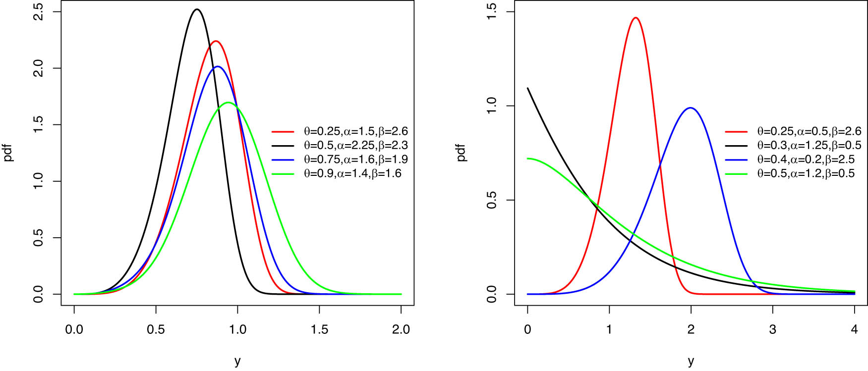
Graphs of the RT-BX density for numerous parameter values.
Next the survival function with the associated hazard rate function of the RT-BX model can be formulated, respectively, by
and
The cumulative, survival, and hazard rate function plots of the RT-BX model are sketched in Figures 2 and 3, respectively. From Figure 3, it can be observed that the hazard rate function increases if
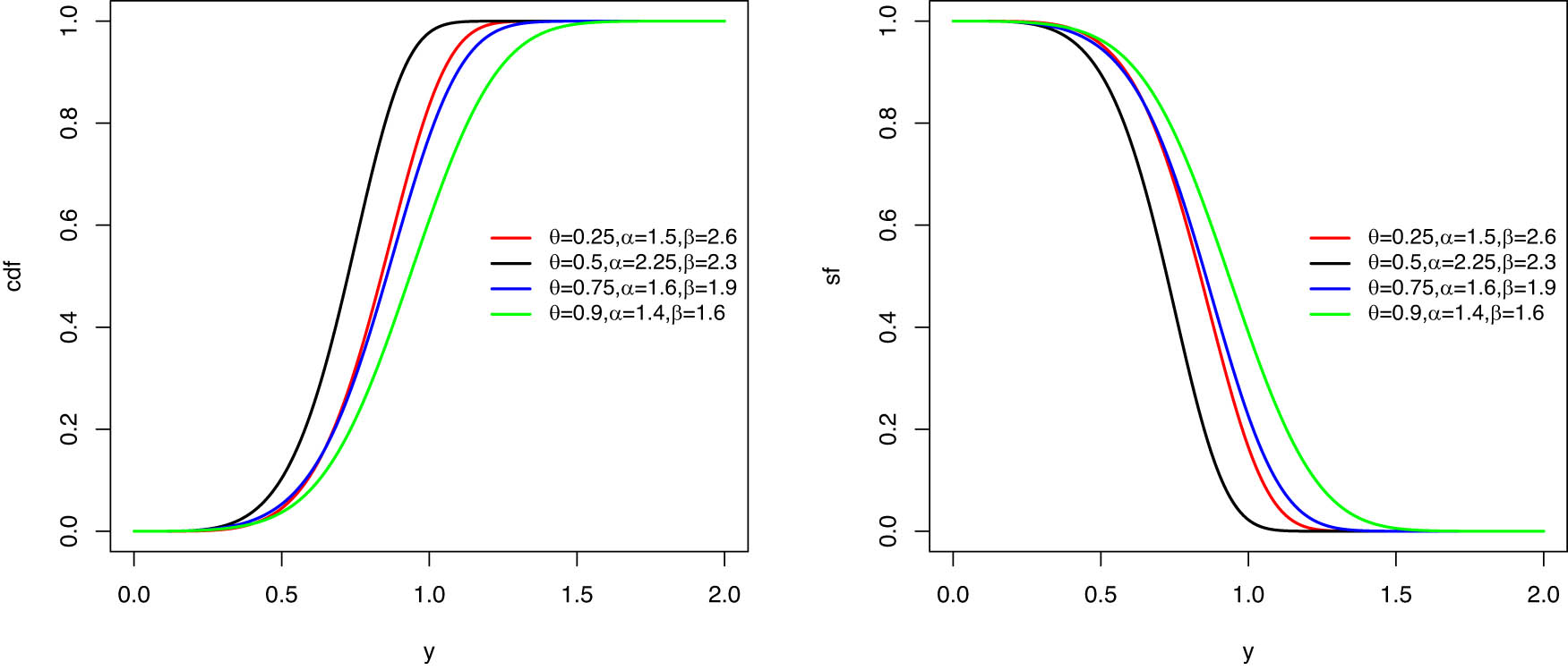
Cumulative and survival plots for the RT-BX model using different values of the parameters.
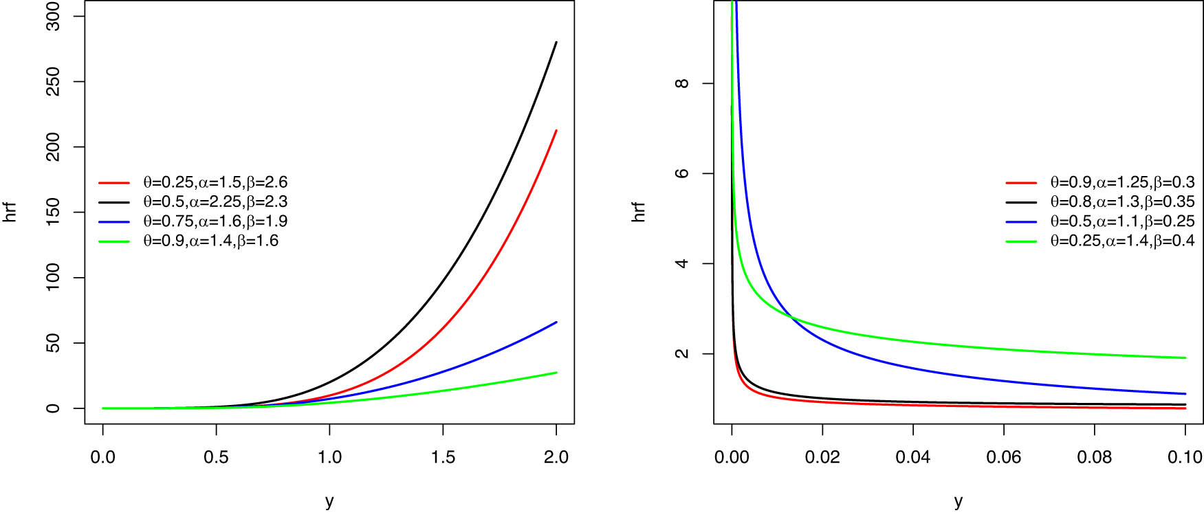
Hazard rate function plots for the RT-BX model using different values of the parameters.
Next the cumulative hazard rate function of the RT-BX is
The reversed hazard rate function can be formulated as
2.2 Behavior of density and hazard rate functions of the RT-BX model
Theorem 1
When
Proof
Put
Based on equation (8), the first derivative of
Clearly, equation (9) is a decreasing function of
which confirms that the function
By using the same steps, if
This ensures that the function
Theorem 2
For
Proof
Let
Hence, from the above equation the function
3 Mathematical properties
We developed here various statistical characteristics of the recommended RT-PBX distribution. From now on, let
3.1 Quantile function of the RT-BX model
The quantile function
Proof
By setting equation (5) equal to
Evidently
which completes the proof. By replacing
The skewness (
and
3.2 Moments with related measures
The kth moment of
where,
Proof
Let
which completes the proof. Consequently, from equation (11), the mean and second-ordered moment of
and
The variance and coefficient of variation (
The moment generating function (MGF) of
The proposed statistical property values of the RT-BX model are tabulated in Tables 1 and 2 by applying various choices of
The findings indicate that
Now,
If
Distinct records of mathematical properties for the RT-BX model at
|
|
|
Var |
|
|
|
|
|---|---|---|---|---|---|---|
|
|
0.5 | 3.0334 | 3.4198 | 0.6096 | 0.8183 | 0.6445 |
| 1 | 1.2038 | 0.5386 | 0.6096 | 0.8183 | 0.6445 | |
| 1.5 | 0.7011 | 0.1827 | 0.6096 | 0.8183 | 0.6445 | |
| 2 | 0.4777 | 0.0848 | 0.6096 | 0.8183 | 0.6445 | |
|
|
0.5 | 1.6533 | 0.3001 | 0.3313 |
|
|
| 1 | 1.0415 | 0.1191 | 0.3313 |
|
|
|
| 1.5 | 0.7948 | 0.0694 | 0.3313 |
|
|
|
| 2 | 0.6561 | 0.0473 | 0.3313 |
|
|
|
|
|
0.5 | 1.3794 | 0.1015 | 0.2310 |
|
|
| 1 | 1.0136 | 0.0548 | 0.2310 |
|
|
|
| 1.5 | 0.8465 | 0.0382 | 0.2310 |
|
|
|
| 2 | 0.7449 | 0.0296 | 0.2310 |
|
|
Distinct records of mathematical properties for the RT-BX model at
|
|
|
Var |
|
|
|
|
|---|---|---|---|---|---|---|
|
|
0.5 | 3.4122 | 3.4976 | 0.5481 | 0.7177 | 0.5191 |
| 1 | 1.3541 | 0.5508 | 0.5481 | 0.7177 | 0.5191 | |
| 1.5 | 0.7886 | 0.1868 | 0.5481 | 0.7177 | 0.5191 | |
| 2 | 0.5374 | 0.0868 | 0.5481 | 0.7177 | 0.5191 | |
|
|
0.5 | 1.7713 | 0.2745 | 0.2958 |
|
|
| 1 | 1.1159 | 0.1089 | 0.2958 |
|
|
|
| 1.5 | 0.8516 | 0.0634 | 0.2958 |
|
|
|
| 2 | 0.7030 | 0.0432 | 0.2958 |
|
|
|
|
|
0.5 | 1.4484 | 0.0886 | 0.2055 |
|
0.2257 |
| 1 | 1.0643 | 0.0478 | 0.2055 |
|
0.2257 | |
| 1.5 | 0.8888 | 0.0334 | 0.2055 |
|
0.2257 | |
| 2 | 0.7822 | 0.0258 | 0.2055 |
|
0.2257 |
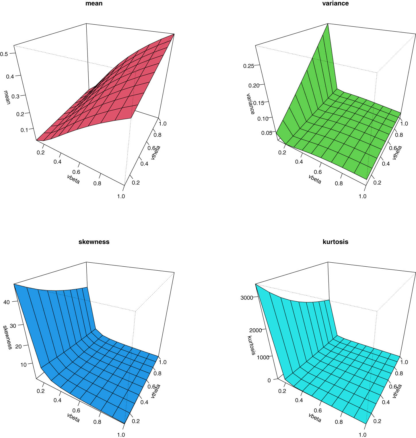
3D curves of proposed statistical measures considering RT-BX with various selected parameter records.
3.3 Order statistics
Let
Consequently, the density for the lowest and highest of
and
4 Entropy information
In this section, numerous information entropies are established. First, the Rényi entropy [29]
Proof
Suppose that
Now, take
which completes the proof.□
Another uncertainty measure is the Shannon entropy [30] (
A new Havrda and Charvat entropy [31] (
Now, the Tsallis entropy [32]
Finally, the Arimoto entropy [33] (
The numerical vales of the suggested entropy information are displayed in Tables 3 and 4 based on numerous selected parameters
Several entropy information records for
|
|
|
|
|
|
|
|
|---|---|---|---|---|---|---|
|
|
0.25 | 4.2854 | 4.1676 | 10.1439 | 7.6772 | 9.5168 |
| 0.75 | 2.0881 | 1.9703 | 3.6228 | 2.7418 | 3.0174 | |
| 1 | 1.5128 | 1.3950 | 2.4293 | 1.8386 | 1.9673 | |
| 1.25 | 1.0665 | 0.9487 | 1.6149 | 1.2222 | 1.2807 | |
|
|
0.25 | 2.1838 | 0.9487 | 3.8385 | 2.9051 | 3.2125 |
| 0.75 | 1.0852 | 0.9487 | 1.6473 | 1.2467 | 1.3075 | |
| 1 | 0.7976 | 0.9487 | 1.1662 | 0.8826 | 0.9136 | |
| 1.25 | 0.5744 | 0.9487 | 0.8162 | 0.6177 | 0.6331 | |
|
|
0.25 | 1.332 | 0.9487 | 2.0885 | 1.5806 | 1.6768 |
| 0.75 | 0.5996 | 0.9487 | 0.8547 | 0.6469 | 0.6637 | |
| 1.25 | 0.4078 | 0.9487 | 0.5673 | 0.4293 | 0.4368 | |
| 1.75 | 0.2591 | 0.9487 | 0.3536 | 0.2676 | 0.2706 |
Several entropy information records for
|
|
|
|
|
|
|
|
|---|---|---|---|---|---|---|
|
|
0.25 | 4.1699 | 4.2913 | 2.9898 | 1.7514 | 2.2527 |
| 0.75 | 1.9727 | 2.0941 | 2.1409 | 1.2541 | 1.4457 | |
| 1 | 1.3973 | 1.5187 | 1.7165 | 1.0055 | 1.1170 | |
| 1.25 | 0.9510 | 1.0724 | 1.2921 | 0.7569 | 0.8150 | |
|
|
0.25 | 2.0443 | 2.1254 | 2.1857 | 1.2804 | 1.4823 |
| 0.75 | 0.9457 | 1.0268 | 1.2864 | 0.7536 | 0.8111 | |
| 1 | 0.6580 | 0.7392 | 0.9572 | 0.5607 | 0.5909 | |
| 1.25 | 0.4349 | 0.5160 | 0.6672 | 0.3908 | 0.4048 | |
|
|
0.25 | 1.1403 | 1.2291 | 1.4837 | 0.8691 | 0.9486 |
| 0.75 | 0.4079 | 0.4967 | 0.6300 | 0.3690 | 0.3814 | |
| 1 | 0.2161 | 0.3049 | 0.3497 | 0.2049 | 0.2085 | |
| 1.25 | 0.0674 | 0.1561 | 0.1131 | 0.0663 | 0.0666 |
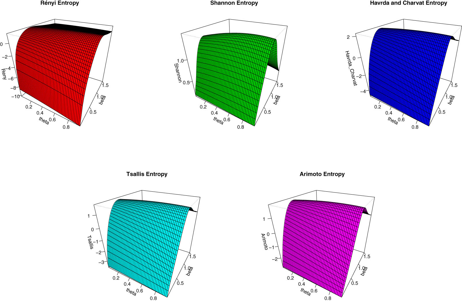
Plots for
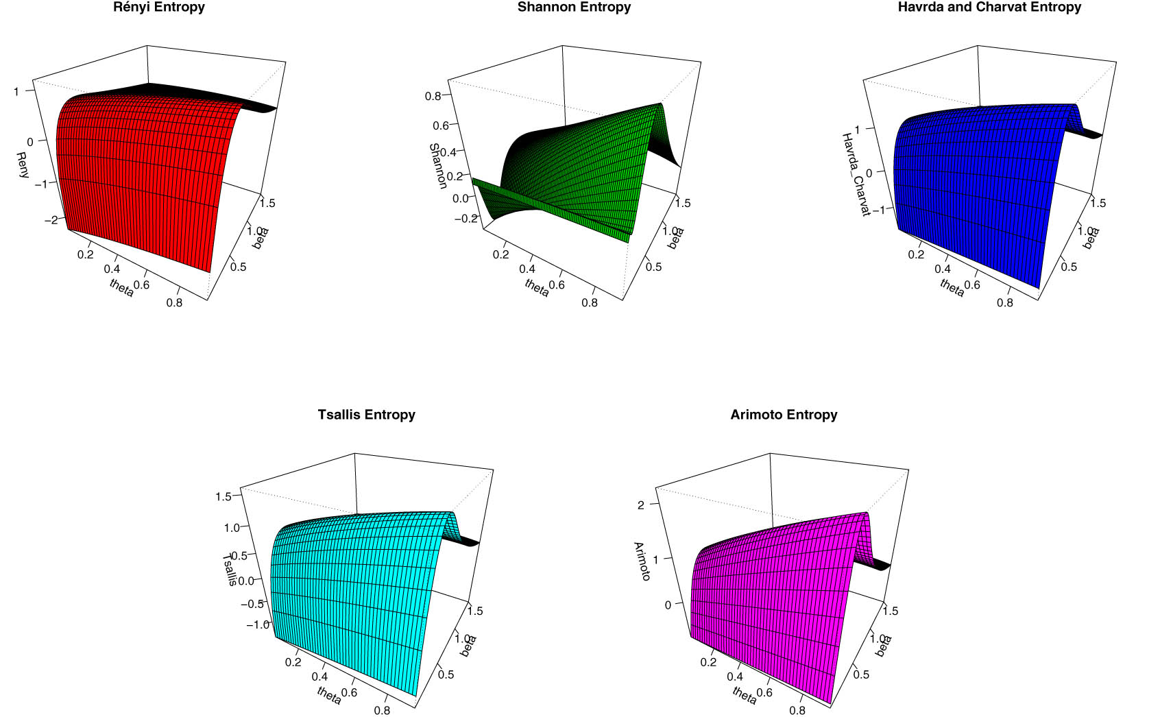
Plots for
5 ML estimator
Let
On solving the below equations, we obtain the estimate of the given parameter of the RT-BX distribution under MLE method.
and
The solution cannot be found analytically and must be obtained using numerical methods. Here in this study, the Newton-Raphson method is commonly applied to obtain the final estimate of the unknown parameters for the RT-BX model numerically.
6 Simulation analysis
In this section, Monte Carlo (MC) simulation studies are conducted to assess the performance of the recommended ML estimator tool for the newly generated RT-BX model by applying numerous sample sizes
Obtain
In the same way, obtain
where
The results of these simulation experiments are reported in Tables 5, 6, 7, 8. Based on the findings presented in Tables 5–8, we can conclude that the final estimates are generally constant and tend to the initial parameters. Also, for all parameter sets, if we increase
Numerical values of the RT-BX model simulation for Set 1
| Sample size | Est. |
|
|
|
|---|---|---|---|---|
| 300 | AE | 0.3776 | 2.2036 | 1.7313 |
| AB | 0.0224 | 0.0464 | 0.0187 | |
| MSE | 0.0748 | 0.0250 | 0.0285 | |
| 500 | AE | 0.3702 | 2.2066 | 1.7441 |
| AB | 0.0218 | 0.0434 | 0.0059 | |
| MSE | 0.0650 | 0.0232 | 0.0219 | |
| 700 | AE | 0.3785 | 2.2114 | 1.7469 |
| AB | 0.0215 | 0.0386 | 0.0031 | |
| MSE | 0.0580 | 0.0185 | 0.0215 | |
| 900 | AE | 0.3859 | 2.2131 | 1.7386 |
| AB | 0.0141 | 0.0369 | 0.0014 | |
| MSE | 0.0522 | 0.0164 | 0.0165 | |
| 1,000 | AE | 0.3941 | 2.2229 | 1.7568 |
| AB | 0.0059 | 0.0271 | 0.0013 | |
| MSE | 0.0461 | 0.0123 | 0.0150 |
Numerical values of the RT-BX model simulation for Set 2
| Sample size | Est. |
|
|
|
|---|---|---|---|---|
| 300 | AE | 0.4210 | 2.1441 | 1.7185 |
| AB | 0.0790 | 0.3559 | 0.2815 | |
| MSE | 0.0916 | 0.0909 | 0.1528 | |
| 500 | AE | 0.4374 | 2.4401 | 2.0159 |
| AB | 0.0626 | 0.0599 | 0.0359 | |
| MSE | 0.0638 | 0.0236 | 0.0926 | |
| 700 | AE | 0.4775 | 2.4701 | 1.9983 |
| AB | 0.0225 | 0.0299 | 0.0217 | |
| MSE | 0.0559 | 0.0167 | 0.0310 | |
| 900 | AE | 0.4816 | 2.4620 | 1.9836 |
| AB | 0.0184 | 0.0280 | 0.0164 | |
| MSE | 0.0460 | 0.0118 | 0.0268 | |
| 1,000 | AE | 0.4836 | 2.4666 | 1.9955 |
| AB | 0.0174 | 0.0234 | 0.0045 | |
| MSE | 0.0373 | 0.0115 | 0.0180 |
Numerical values of the RT-BX model simulation for Set 3
| Sample size | Est. |
|
|
|
|---|---|---|---|---|
| 300 | AE | 0.5693 | 2.6216 | 2.1687 |
| AB | 0.0307 | 0.1284 | 0.0813 | |
| MSE | 0.0747 | 0.2479 | 0.2110 | |
| 500 | AE | 0.5710 | 2.722 | 2.2628 |
| AB | 0.0290 | 0.0480 | 0.0428 | |
| MSE | 0.0553 | 0.1148 | 0.0827 | |
| 700 | AE | 0.5759 | 2.7183 | 2.2553 |
| AB | 0.0241 | 0.0317 | 0.0383 | |
| MSE | 0.0460 | 0.0377 | 0.0465 | |
| 900 | AE | 0.5845 | 2.7238 | 2.2706 |
| AB | 0.0155 | 0.0262 | 0.0206 | |
| MSE | 0.0397 | 0.0111 | 0.0347 | |
| 1,000 | AE | 0.5925 | 2.7224 | 2.2585 |
| AB | 0.0150 | 0.0226 | 0.0085 | |
| MSE | 0.0304 | 0.0077 | 0.0276 |
Numerical values of the RT-BX model simulation for Set 4
| Sample size | Est. |
|
|
|
|---|---|---|---|---|
| 300 | AE | 0.7052 | 2.9877 | 2.5768 |
| AB | 0.0448 | 0.0923 | 0.0768 | |
| MSE | 0.0473 | 0.0808 | 0.0952 | |
| 500 | AE | 0.7365 | 2.9586 | 2.5387 |
| AB | 0.0135 | 0.04140 | 0.0387 | |
| MSE | 0.0464 | 0.0659 | 0.0687 | |
| 700 | AE | 0.7405 | 2.9863 | 2.5316 |
| AB | 0.0095 | 0.01370 | 0.0316 | |
| MSE | 0.0405 | 0.0148 | 0.0557 | |
| 900 | AE | 0.7481 | 2.9901 | 2.5224 |
| AB | 0.0079 | 0.0099 | 0.0224 | |
| MSE | 0.0375 | 0.0088 | 0.0484 | |
| 1,000 | AE | 0.7494 | 2.9982 | 2.5686 |
| AB | 0.0306 | 0.0018 | 0.0186 | |
| MSE | 0.00578 | 0.0066 | 0.0446 |
7 Data analysis
Here we applied three real-life data sets to see the applicability, flexibility, and potentiality of the proposed RT-BX distribution. We apply the same data sets to compare the suggested model with the BX, transmuted log normal (T-LN), transmuted Weibul (T-Wei), transmuted log logistic (T-LL), and Extended exponential (Ex-Exp) distributions. Most of those models have received great attention in modeling several fields of data sets. It is often useful and necessary to check whether the considered model fit the data properly or not, and therefore, we use different standard metrics including the estimation of parameters, Kolmogorov-Smirnov (
Distribution performance and information criterion values based on given three data sets
| Data | Distribution |
|
|
|
|
|
|
|
|---|---|---|---|---|---|---|---|---|
| RT-BX | 0.5551 | 0.2993 | 1.1546 | 0.1078 | 0.7402 | 141.668 | 146.734 | |
| BX | 0.2090 | 1.2555 | 0.1281 | 0.5272 | 143.363 | 146.741 | ||
| T-LN |
|
0.7873 | 0.6498 | 0.1656 | 0.2225 | 156.596 | 161.663 | |
| 1 | T-Wei |
|
2.3622 | 3.222 | 0.1108 | 0.7095 | 142.411 | 147.478 |
| T-LL |
|
3.0599 | 0.3598 | 0.1661 | 0.2197 | 157.563 | 162.630 | |
| Ex-Exp | 0.6228 | 3.5734 | 0.1657 | 0.2216 | 156.853 | 161.23 | ||
| RT-BX | 0.7044 | 0.4257 | 2.3571 | 0.1412 | 0.1620 | 34.552 | 40.981 | |
| BX | 0.2745 | 2.6809 | 0.1744 | 0.0432 | 38.960 | 42.247 | ||
| T-LN |
|
0.2983 | 0.2610 | 0.2075 | 0.0087 | 56.300 | 62.729 | |
| 1 | T-Wei |
|
4.7418 | 1.5204 | 0.1522 | 0.1078 | 35.070 | 41.50 |
| T-LL |
|
6.0109 | 0.7142 | 0.1745 | 0.0430 | 39.030 | 42.559 | |
| Ex-Exp | 2.6118 | 31.357 | 0.2290 | 0.0026 | 66.767 | 71.053 | ||
| RT-BX | 0.4467 | 0.4387 | 0.5598 | 0.0839 | 0.7244 | 377.838 | 384.496 | |
| BX | 0.3260 | 0.6124 | 0.0886 | 0.6593 | 377.934 | 384.779 | ||
| T-LN |
|
1.0099 | 1.1304 | 0.1421 | 0.1278 | 391.477 | 398.136 | |
| 3 | T-Wei |
|
1.0684 | 4.9840 | 0.0912 | 0.6225 | 378.221 | 384.880 |
| T-LL |
|
1.6762 | 0.2538 | 0.0983 | 0.5260 | 381.345 | 387.004 | |
| Ex-Exp | 0.2020 | 1.3144 | 0.1079 | 0.4064 | 387.669 | 392.108 |
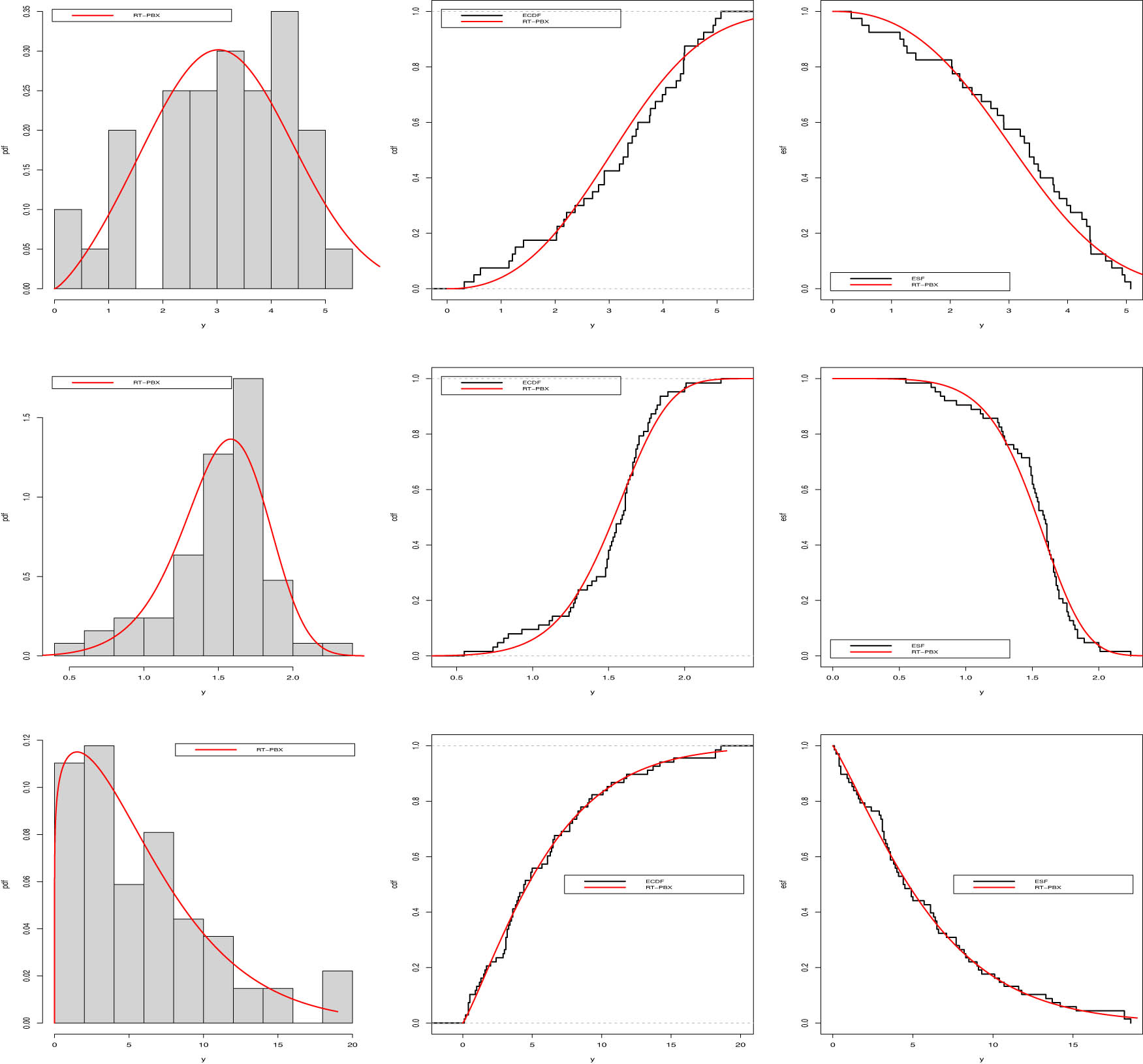
Estimated density, cumulative distribution, and survival function of the RT-BX model by applying the three considered data sets.
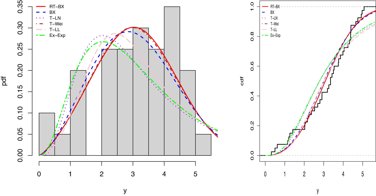
Estimated density, cdf plots for fitting proposed models using first data set.
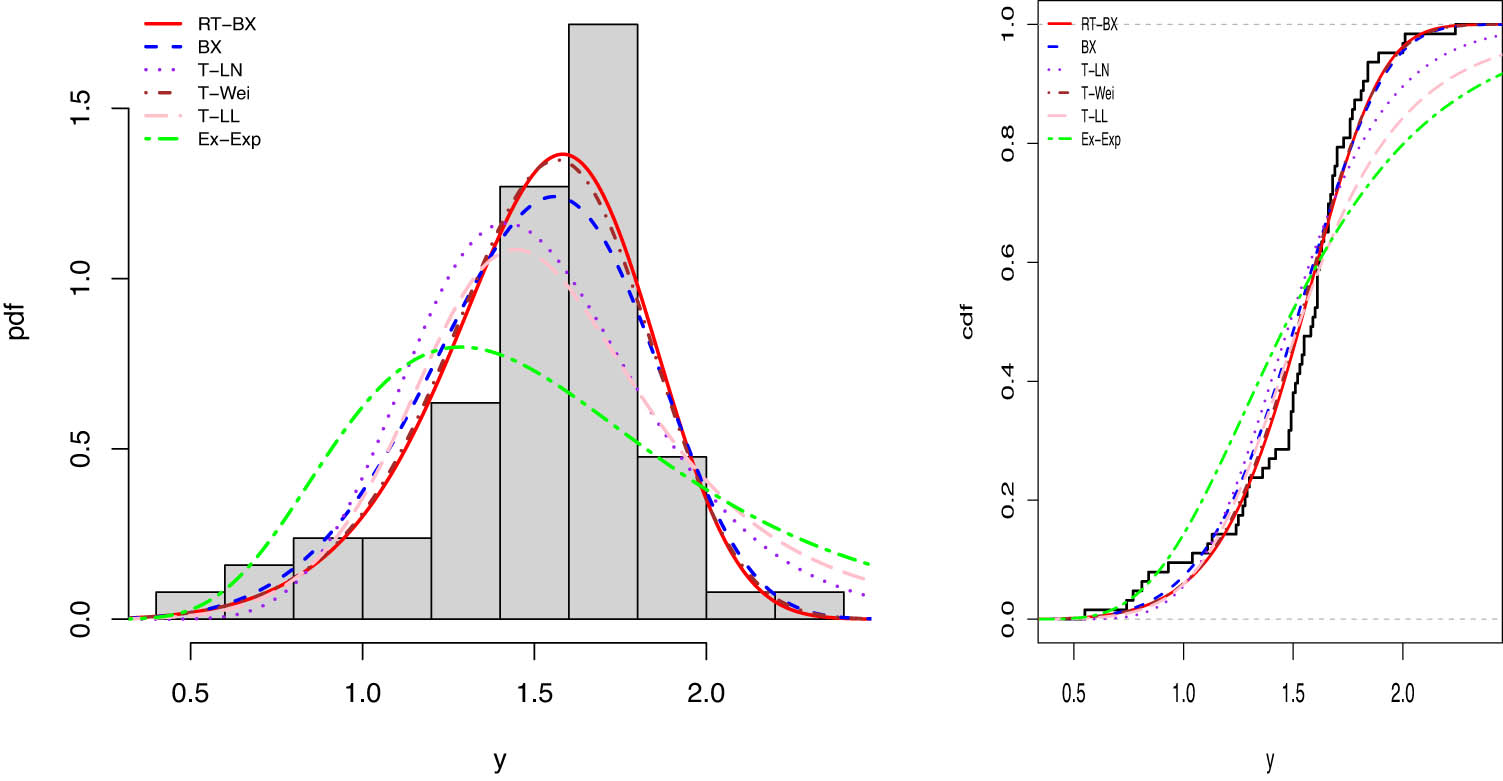
Estimated density, cdf plots for fitting proposed models using second data set.
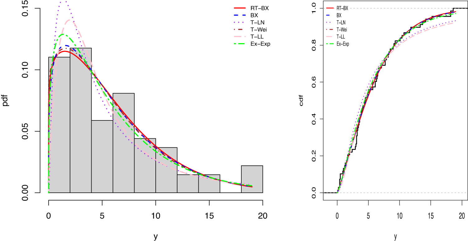
Estimated density, cdf plots for fitting proposed models using third data set.
7.1 First data set
The first data set was reported by Alshawarbeh et al. [34] and it represents 40 leukemia patients drawn from Saudi Arabia health ministry hospital. The values of the proposed data set are shown in Table 10.
Values of data set 1
| 0.315 | 0.496 | 0.616 | 1.145 | 1.208 | 1.263 | 1.414 | 2.025 | 2.036 | 2.162 |
| 2.211 | 2.370 | 2.532 | 2.693 | 2.805 | 2.910 | 2.912 | 3.192 | 3.263 | 3.348 |
| 3.348 | 3.427 | 3.499 | 3.534 | 3.767 | 3.751 | 3.858 | 3.986 | 4.049 | 4.244 |
| 4.323 | 4.381 | 4.392 | 4.397 | 4.647 | 4.753 | 4.929 | 4.973 | 5.074 | 4.381 |
7.2 Second data set
Here this data set contains 63 values and considered the strengths of 1.5 cm glass fibers. The suggested data set is applied by Smith and Naylor [35] and it is summarized in Table 11.
Values of the strengths of 1.5 cm glass fibers
| 0.55 | 0.93 | 1.25 | 1.36 | 1.49 | 1.52 | 1.58 | 1.61 | 1.64 | 1.68 |
| 1.73 | 1.81 | 2 | 0.74 | 1.04 | 1.27 | 1.53 | 1.59 | 1.61 | 1.66 |
| 1.68 | 1.76 | 1.82 | 2.01 | 0.77 | 1.11 | 1.28 | 1.42 | 1.5 | 1.54 |
| 1.6 | 1.62 | 1.76 | 1.84 | 2.24 | 0.81 | 1.13 | 1.29 | 1.48 | 1.5 |
| 1.55 | 1.61 | 1.62 | 1.66 | 1.7 | 1.77 | 1.84 | 0.84 | 1.48 | 1.51 |
| 1.55 | 1.61 | 1.63 | 1.67 | 1.7 | 1.78 | 1.89 | 1.39 | 1.49 | 1.66 |
| 1.69 | 1.24 | 1.3 |
7.3 Third data set
The source of this data is taken from Patil and Rao [36] as well as Almetwally and Meraou provide it [37]. The proposed data set represents the locations of the 68 stakes found while walking
Sixty eight stakes found while walking and looking data set
| 2.0 | 0.5 | 10.4 | 3.6 | 0.9 | 1.0 | 3.4 | 2.9 | 8.2 | 6.5 | 5.7 | 3.0 | 4.0 |
| 0.1 | 11.8 | 14.2 | 2.4 | 1.6 | 13.3 | 6.5 | 8.3 | 4.9 | 1.5 | 18.6 | 0.4 | 0.4 |
| 0.2 | 11.6 | 3.2 | 7.1 | 10.7 | 3.9 | 6.1 | 6.4 | 3.8 | 15.2 | 3.5 | 3.1 | 7.9 |
| 18.2 | 10.1 | 4.4 | 1.3 | 13.7 | 6.3 | 3.6 | 9.0 | 7.7 | 4.9 | 9.1 | 3.3 | 8.5 |
| 6.1 | 0.4 | 9.3 | 0.5 | 1.2 | 1.7 | 4.5 | 3.1 | 3.1 | 6.6 | 4.4 | 5.0 | 3.2 |
| 7.7 | 18.2 | 4.1 |
Table 13 shows the numerous basic statistics of the observed data sets, and Figure 11 displays the numerous non-parametric plots notably the scaled total time on the test (TTT), the probability-probability (PP), and box plots.
Basic mathematical measures for the three suggested data
| Data | Min |
|
|
|
|
Max |
|
|
|---|---|---|---|---|---|---|---|---|
| 1 | 0.315 | 2.199 | 3.348 | 3.116 | 4.264 | 5.074 |
|
|
| 2 | 0.550 | 1.375 | 1.590 | 1.507 | 1.685 | 2.240 |
|
0.8001 |
| 3 | 0.100 | 2.975 | 4.450 | 5.853 | 8.225 | 18.600 | 1.020 | 0.470 |
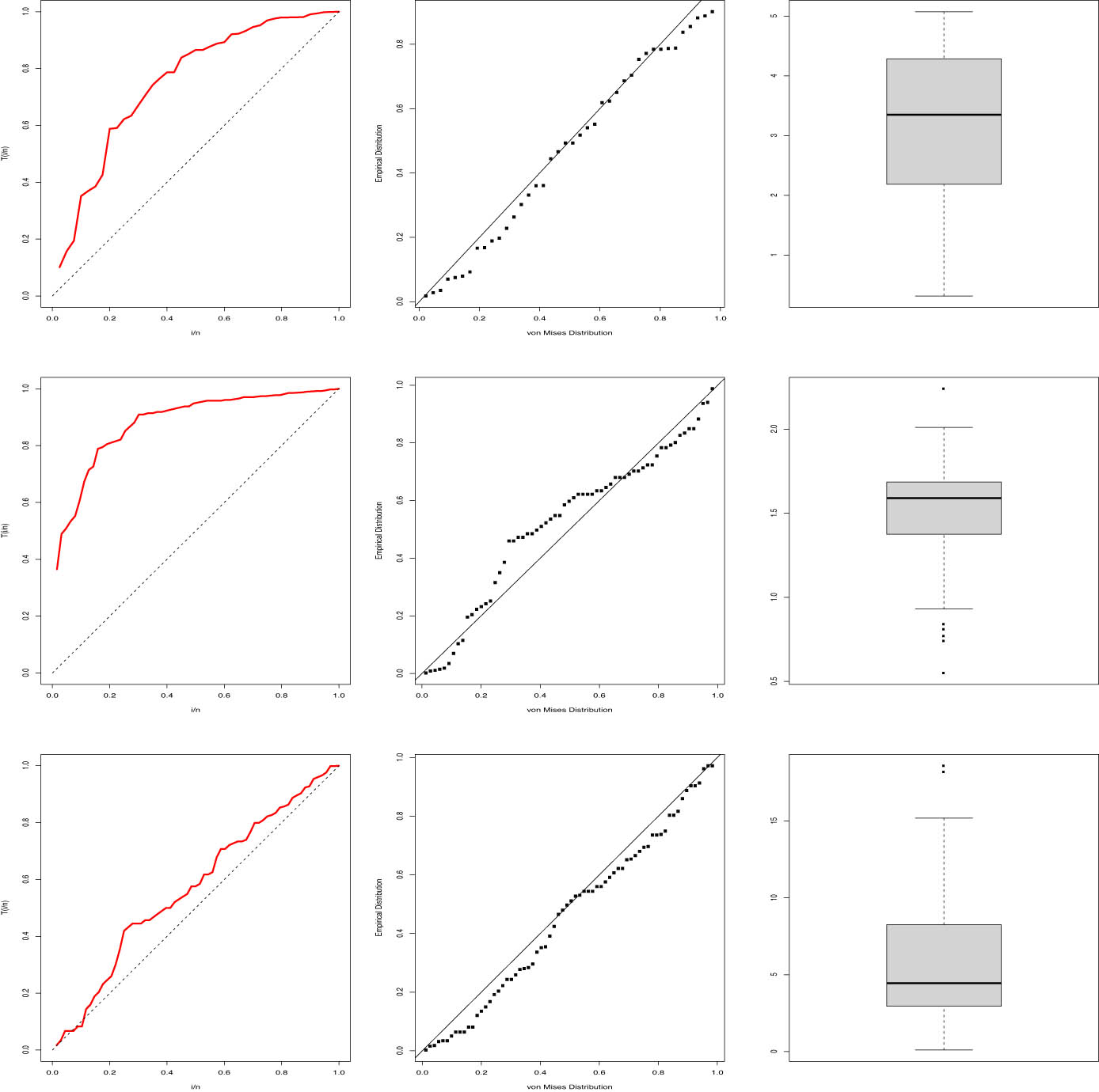
TTT, PP, and box plots for the selected data sets.
8 Conclusion
A novel approach to BXD is defined in this work using a record-based transmuted tool, which is a powerful tool in modeling numerous types of data sets, notably skewed, complex, asymmetric, and symmetric. The recommended model has three parameters, and its density has different shapes. Further, we provide the maximum likelihood approach for estimating the model parameters, as well as several simulation experiments are performed to demonstrate the efficiency of the suggested estimation technique. At the end, the applicability of the proposed distribution is demonstrated using three real data sets. The obtained results illustrate that our recommended model is the best fitting distribution for fitting the three recommended data sets.
-
Funding information: The author states no funding involved.
-
Author contributions: The author confirms the sole responsibility for the conception of the study, presented results, and manuscript preparation.
-
Conflict of interest: The author states no conflicts of interest.
-
Data availability statement: All data sets used in this study are contained in this article.
References
[1] G. Hamedani, M. Korkmaz, N. Butt, and H. Yousof, The type II quasi Lambert family: properties, characterizations and different estimation methods, Pak. J. Stat. Oper. Res. 18 (2022), no. 4, 963–983, DOI: https://doi.org/10.18187/pjsor.v18i4.3907. 10.18187/pjsor.v18i4.3907Search in Google Scholar
[2] M. Cordeiro and R. Brito, The beta power distribution, Braz. J. Probab. Stat. 26 (2012), no. 1, 88–112, DOI: http://dx.doi.org/10.1214/10-BJPS124. 10.1214/10-BJPS124Search in Google Scholar
[3] A. Marshall and I. Olkin, A new method for adding a parameter to a family of distributions with application to the exponential and Weibull families, Biometrika 84 (1997), no. 3, 641–652, DOI: https://doi.org/10.1093/biomet/84.3.641. 10.1093/biomet/84.3.641Search in Google Scholar
[4] A. Mahdavi and D. Kundu, A new method for generating distributions with an application to exponential distribution, Comm. Statist. Theory Methods 46 (2017), no. 13, 6543–6557, DOI: https://doi.org/10.1080/03610926.2015.1130839. 10.1080/03610926.2015.1130839Search in Google Scholar
[5] A. Hassan, R. Mohamd, M. Elgarhy, and A. Fayomi, Alpha power transformed extended exponential distribution: properties and applications, J. Nonlinear Sci. Appl. 12 (2018), no. 4, 62–67, DOI: http://dx.doi.org/10.22436/jnsa.012.04.05. 10.22436/jnsa.012.04.05Search in Google Scholar
[6] T. Moakofi, B. Oluyede, and F. Chipepa, Type II exponentiated half-logistic Topp-Leone Marshall-Olkin-G family of distributions with applications, Heliyon 7 (2021), no. 12, e08590. 10.1016/j.heliyon.2021.e08590Search in Google Scholar PubMed PubMed Central
[7] J. Eghwerido, S, Zelibe, and E. Efe-Eyefia, Gompertz-alpha power inverted exponential distribution: properties and applications, Thail. Stat. 18 (2020), no. 3, 319–332, https://ph02.tci-thaijo.org/index.php/thaistat/article/view/241282. Search in Google Scholar
[8] L. Sapkota, V. Kumar, A. Gemeay, M. Bakr, O. Balogun, and A. Muse, New Lomax-G family of distributions: Statistical properties and applications, AIP Adv. 13 (2023), no. 9, 095128, DOI: https://doi.org/10.1063/5.0171949. 10.1063/5.0171949Search in Google Scholar
[9] M. Meraou and M. Raqab, Statistical properties and different estimation procedures of Poisson Lindley distribution, J. Stat. Theory Appl. 20 (2021), no. 1, 33–45, DOI: https://doi.org/10.2991/jsta.d.210105.001. 10.2991/jsta.d.210105.001Search in Google Scholar
[10] M. Meraou, N. Al-Kandari, M. Raqab, and D. Kundu, Analysis of skewed data by using compound Poisson exponential distribution with applications to insurance claims, J. Stat. Comput. Simul. 92 (2021), no. 5, 928–956, DOI: https://doi.org/10.1080/00949655.2021.1981324. 10.1080/00949655.2021.1981324Search in Google Scholar
[11] B. Thomas and V. Chacko, Power generalized DUS transformation in Weibull and Lomax distributions, Reliability: Theory & Applications 1 (2023), no. 72, 368–384. Search in Google Scholar
[12] N. Balakrishnan and M. He, A record-based transmuted family of distributions, in: I. Ghosh, N. Balakrishnan, H. K. T. Ng (Eds.), Advances in Statistics Theory and Applications, Emerging Topics in Statistics and Biostatistics, Springer, Cham, Switzerland, 2021, pp. 3–24, DOI: https://doi.org/10.1007/978-3-030-62900-7_1. 10.1007/978-3-030-62900-7_1Search in Google Scholar
[13] C. Tanis and B. Saracoglu, On the record-based transmuted model of Balakrishnan and He based on Weibull distribution, Comm. Statist. Simulation Comput. 51 (2022), no. 8, 4204–4224, DOI: https://doi.org/10.1080/03610918.2020.1740261. 10.1080/03610918.2020.1740261Search in Google Scholar
[14] M. Arshad, M. Khetan, V. Kumar, and A. Pathak, Record-based transmuted generalized linear exponential distribution with increasing, decreasing and bathtub shaped failure rates, Comm. Statist. Simulation Comput. 53 (2022), no. 7, 1–25, DOI: https://doi.org/10.1080/03610918.2022.2106494. 10.1080/03610918.2022.2106494Search in Google Scholar
[15] C. Tanis, A new Lindley distribution: applications to COVID-19 patients data, Soft Comput. 28 (2024), 2863–2874, DOI: https://doi.org/10.1007/s00500-023-09339-7. 10.1007/s00500-023-09339-7Search in Google Scholar
[16] K. Sakthivel and V. Nandhini, Record-based transmuted power Lomax distribution: properties and its applications in reliability, Reliability: Theory & Applications 17 (2022), no. 4, 574–592. Search in Google Scholar
[17] A. L. Sobhi and M. Mashail, Moments of dual generalized order statistics and characterization for transmuted exponential model, Comput. J. Math. Stat. Sci. 1 (2022), no. 1, 42–50. 10.21608/cjmss.2022.272548Search in Google Scholar
[18] R. A. Mohamed, I. Elbatal, E. M. ALmetwally, M. Elgarhy, and H. M. Almongy, Bayesian estimation of a transmuted Topp-Leone length biased exponential model based on competing risk with the application of electrical appliances, Mathematics 10 (2022), no. 21, 4042. 10.3390/math10214042Search in Google Scholar
[19] V. Kumar, A. Chakraborty, M. Arshad, and A. Tiwari, A new Nadarajah-Haghighi distribution with applications, Res. Square 1 (2024), DOI: https://doi.org/10.21203/rs.3.rs-3825940/v1. 10.21203/rs.3.rs-3825940/v1Search in Google Scholar
[20] R. Usman and M. Ilyas, The power Burr Type X distribution: properties, regression modeling and applications, Punjab Univ. J. Math. 52 (2020), 27–44. Search in Google Scholar
[21] A. A. Al-Babtain, I. Elbatal, H. Al-Mofleh, A. M. Gemeay, A. Z. Afify, and A. M. Sarg, The flexible Burr XG family: properties, inference, and applications in engineering science, Symmetry 13 (2021), no. 3, 474. 10.3390/sym13030474Search in Google Scholar
[22] A. Fayomi, A. Hassan, H. Baaqeel, and E. Almetwally, Bayesian inference and data analysis of the unit-power Burr X distribution, Axioms 2023 (2023), no. 12, 297, DOI: https://doi.org/10.3390/axioms12030297. 10.3390/axioms12030297Search in Google Scholar
[23] M. Raqab and D. Kundu, Burr type X distribution: revisited, J. Probab. Stat. Sci. 4 (2006), 179–193. Search in Google Scholar
[24] E. Yıldırım, E. Ilıkkan, A. Gemeay, N. Makumi, M. Bakr, and O. Balogun, Power unit Burr-XII distribution: Statistical inference with applications, AIP Adv. 13 (2023), no. 10, 105107.10.1063/5.0171077Search in Google Scholar
[25] M. Korkmaz, E. Altun, H. Yousof, A. Afify, and S. Nadarajah, The Burr X Pareto distribution: properties, applications and VaR estimation, J. Risk Financial Manag. 11 (2018), no. 1, 1–16, DOI: https://doi.org/10.3390/jrfm11010001. 10.3390/jrfm11010001Search in Google Scholar
[26] F. Merovci, M. Khaleel, and N. Ibrahim, The beta Burr type X distribution properties with application, SpringerPlus 5 (2016), no. 697, 1–18, DOI: https://doi.org/10.1186/s40064-016-2271-9. 10.1186/s40064-016-2271-9Search in Google Scholar PubMed PubMed Central
[27] J. G. Surles and W. J. Padgett, Some properties of a scaled Burr type X distribution, Inference 128 (2005), no. 1, 271–280, DOI: https://doi.org/10.1016/j.jspi.2003.10.003. 10.1016/j.jspi.2003.10.003Search in Google Scholar
[28] R. Glaser, Bathtub and related failure rate characterizations, J. Amer. Statist. Assoc. 75 (1980), no. 371, 667–672, DOI: https://doi.org/10.1080/01621459.1980.10477530. 10.1080/01621459.1980.10477530Search in Google Scholar
[29] A. Rényi, On measures of entropy and information, in: Proceedings 4th Berkeley Symposium on Mathematical Statistics and Probability, University of California Press, 1960. Search in Google Scholar
[30] C. Shannon, A mathematical theory of communication, Bell Syst. Tech. J. 27 (1948), 379–423, DOI: https://doi.org/10.1002/j.1538-7305.1948.tb01338.x. 10.1002/j.1538-7305.1948.tb01338.xSearch in Google Scholar
[31] J. Havrda and F. Charvat, Quantification method of classification processes: concept of structural-entropy, Kybernetika 3 (1967), no. 1, 30–35, DOI: http://eudml.org/doc/28681. Search in Google Scholar
[32] C. Tsallis, Possible generalization of Boltzmann-Gibbs statistics, J. Stat. Phys. 52 (1988), no. 1–2, 479–487, DOI: https://doi.org/10.1007/BF01016429. 10.1007/BF01016429Search in Google Scholar
[33] S. Arimoto, Information-theoretical considerations on estimation problems, Inf. Control 19 (1971), no. 3, 181–194, DOI: https://doi.org/10.1016/S0019-9958(71)90065-9. 10.1016/S0019-9958(71)90065-9Search in Google Scholar
[34] E. Alshawarbeh, M. Z. Arshad, M. Z. Iqbal, M. Ghamkhar, A. Al Mutairi, M. A. Meraou, et al., Modeling medical and engineering data using a new power function distribution: theory and inference, J. Radiat. Res. Appl. Sci. 17 (2024), no. 1, 1–15, DOI: https://doi.org/10.1016/j.jrras.2023.10078710.1016/j.jrras.2023.100787Search in Google Scholar
[35] R. Smith and J. Naylor, A comparison of maximum likelihood and Bayesian estimators for three-parameter Weibull distribution, Appl. Stat. 36 (1987), 358–369, DOI: https://doi.org/10.2307/2347795. 10.2307/2347795Search in Google Scholar
[36] G. Patil and C. Rao, Environmental Statistics, Handbook of Statistics, vol. 12, Elsevier B.V., 1994. Search in Google Scholar
[37] E. Almetwally and M. Meraou, Application of environmental data with new extension of Nadarajah-Haghighi distribution, Comput. J. Math. Stat. Sci. 1 (2022), no. 1, 26–41, DOI: https://doi.org/10.21608/cjmss.2022.271186. 10.21608/cjmss.2022.271186Search in Google Scholar
© 2025 the author(s), published by De Gruyter
This work is licensed under the Creative Commons Attribution 4.0 International License.
Articles in the same Issue
- Special Issue on Contemporary Developments in Graphs Defined on Algebraic Structures
- Forbidden subgraphs of TI-power graphs of finite groups
- Finite group with some c#-normal and S-quasinormally embedded subgroups
- Classifying cubic symmetric graphs of order 88p and 88p 2
- Simplicial complexes defined on groups
- Two-sided zero-divisor graphs of orientation-preserving and order-decreasing transformation semigroups
- Further results on permanents of Laplacian matrices of trees
- Special Issue on Convex Analysis and Applications - Part II
- A generalized fixed-point theorem for set-valued mappings in b-metric spaces
- Research Articles
- Dynamics of particulate emissions in the presence of autonomous vehicles
- The regularity of solutions to the Lp Gauss image problem
- Exploring homotopy with hyperspherical tracking to find complex roots with application to electrical circuits
- The ill-posedness of the (non-)periodic traveling wave solution for the deformed continuous Heisenberg spin equation
- Some results on value distribution concerning Hayman's alternative
- 𝕮-inverse of graphs and mixed graphs
- A note on the global existence and boundedness of an N-dimensional parabolic-elliptic predator-prey system with indirect pursuit-evasion interaction
- On a question of permutation groups acting on the power set
- Chebyshev polynomials of the first kind and the univariate Lommel function: Integral representations
- Blow-up of solutions for Euler-Bernoulli equation with nonlinear time delay
- Spectrum boundary domination of semiregularities in Banach algebras
- Statistical inference and data analysis of the record-based transmuted Burr X model
- A modified predictor–corrector scheme with graded mesh for numerical solutions of nonlinear Ψ-caputo fractional-order systems
- Dynamical properties of two-diffusion SIR epidemic model with Markovian switching
- Classes of modules closed under projective covers
- On the dimension of the algebraic sum of subspaces
- Periodic or homoclinic orbit bifurcated from a heteroclinic loop for high-dimensional systems
- On tangent bundles of Walker four-manifolds
- Regularity of weak solutions to the 3D stationary tropical climate model
- A new result for entire functions and their shifts with two shared values
- Freely quasiconformal and locally weakly quasisymmetric mappings in metric spaces
- On the spectral radius and energy of the degree distance matrix of a connected graph
- Solving the quartic by conics
- A topology related to implication and upsets on a bounded BCK-algebra
- On a subclass of multivalent functions defined by generalized multiplier transformation
- Local minimizers for the NLS equation with localized nonlinearity on noncompact metric graphs
- Approximate multi-Cauchy mappings on certain groupoids
- Multiple solutions for a class of fourth-order elliptic equations with critical growth
- A note on weighted measure-theoretic pressure
- Majorization-type inequalities for (m, M, ψ)-convex functions with applications
- Recurrence for probabilistic extension of Dowling polynomials
- Unraveling chaos: A topological analysis of simplicial homology groups and their foldings
- Global existence and blow-up of solutions to pseudo-parabolic equation for Baouendi-Grushin operator
- A characterization of the translational hull of a weakly type B semigroup with E-properties
- Some new bounds on resolvent energy of a graph
- Carmichael numbers composed of Piatetski-Shapiro primes in Beatty sequences
- The number of rational points of some classes of algebraic varieties over finite fields
- Singular direction of meromorphic functions with finite logarithmic order
- Pullback attractors for a class of second-order delay evolution equations with dispersive and dissipative terms on unbounded domain
- Eigenfunctions on an infinite Schrödinger network
- Boundedness of fractional sublinear operators on weighted grand Herz-Morrey spaces with variable exponents
- On SI2-convergence in T0-spaces
- Bubbles clustered inside for almost-critical problems
- Classification and irreducibility of a class of integer polynomials
- Existence and multiplicity of positive solutions for multiparameter periodic systems
- Averaging method in optimal control problems for integro-differential equations
- On superstability of derivations in Banach algebras
- Investigating the modified UO-iteration process in Banach spaces by a digraph
- The evaluation of a definite integral by the method of brackets illustrating its flexibility
- Existence of positive periodic solutions for evolution equations with delay in ordered Banach spaces
- Tilings, sub-tilings, and spectral sets on p-adic space
- The higher mapping cone axiom
- Continuity and essential norm of operators defined by infinite tridiagonal matrices in weighted Orlicz and l∞ spaces
-
A family of commuting contraction semigroups on
- Pullback attractor of the 2D non-autonomous magneto-micropolar fluid equations
- Maximal function and generalized fractional integral operators on the weighted Orlicz-Lorentz-Morrey spaces
- On a nonlinear boundary value problems with impulse action
- Normalized ground-states for the Sobolev critical Kirchhoff equation with at least mass critical growth
- Decompositions of the extended Selberg class functions
- Subharmonic functions and associated measures in ℝn
- Some new Fejér type inequalities for (h, g; α - m)-convex functions
- The robust isolated calmness of spectral norm regularized convex matrix optimization problems
- Multiple positive solutions to a p-Kirchhoff equation with logarithmic terms and concave terms
- Joint approximation of analytic functions by the shifts of Hurwitz zeta-functions in short intervals
- Green's graphs of a semigroup
- Some new Hermite-Hadamard type inequalities for product of strongly h-convex functions on ellipsoids and balls
- Infinitely many solutions for a class of Kirchhoff-type equations
- On an uncertainty principle for small index subgroups of finite fields