A modified predictor–corrector scheme with graded mesh for numerical solutions of nonlinear Ψ-caputo fractional-order systems
-


Abstract
The aim of this article is to develop a modified predictor–corrector scheme for solving the system of nonlinear
1 Introduction
Over the last few decades, the concepts of fractional calculus have increased interest in related fields of science and engineering. Some important results in applications of fractional calculus are reported in [1]. Additionally, fractional calculus can be described as complex procedures in real world applications such as signal and image processing [2], biology [3], environmental science [4], economics [5], multidisciplinary engineering fields [6], etc. In mathematical models, fractional derivatives are suitable tools for explaining memory and hereditary properties of several materials and processes. Moreover, there are many definitions of fractional derivatives for applying to fractional-order models, e.g., Caputo-Hadamard, Hadamard, Caputo-Erdélyi-Kober, Erdélyi-Kober, Caputo, and Riemann-Liouville. We recommend reading previous studies [7–10] for further information.
There is a specific type of kernel dependency represented in each of those definitions. To investigate fractional differential equations in a comprehensive way, Almeida [11] proposed the definition of fractional derivatives with arbitrary kernel and called
The study of
To extend the idea of Almeida et al. [16], solving the system of nonlinear
where
This work is divided to six sections as follows. The first section is introduction. It includes the review of the related research and work. In Section 2, important definitions for the system of fractional differential equations with
2
Ψ
-Caputo nonlinear fractional-order systems
Some definitions and theorems in this section will be used to declare and verify our essential results. Let
Definition 2.1
[8] The Riemann-Liouville fractional integral of the function
where
Definition 2.2
[11] The
Definition 2.3
[11] Let
Definition 2.4
[12] Given
where
Remark 1
From Definition 2.4, the examples of specific kernels
Then, the important properties of fractional
Theorem 2.1
[12] If
and
In this study, the
where
The function
or
Based on the idea of Songsanga and Sa Ngiamsunthorn [23], we extend the concept of predictor–corrector scheme for solving
2.1 Smoothness properties
Theorem 2.2
[22]
Assume that
where
Assume that
where
Additionally, we applied Theorem 2.2 and modified the smoothness assumptions of [22] to the solution of
Assumption 1
Given
where
Let
Therefore, condition (9) can be rewritten as follows:
Remark 2
Assumption 1 provides the behavior of
3 Predictor-corrector scheme with graded mesh
In this section, we investigate the predictor–corrector scheme for solving the system of nonlinear fractional differential equations involving
To divide the partition on the interval
where
The predictor–corrector scheme is proposed in the work of Liu et al. [22] for solving the numerical solution of nonlinear fractional differential equations. It is suggested to be one of the most reliable, consistent, and effective approaches. The graded mesh is applied to recover the optimal convergence order for Volterra integral equations. The SVIEs (13) can be solved through the modification of predictor–corrector scheme with graded mesh [22]. To approximate
where
Next the function
Then, this step is called corrector step and is defined as
where
Therefore, the predictor–corrector scheme is defined as
where
4 Error estimation of the approximation
Next we introduce some properties of the coefficients in (15) and (18), respectively, and several useful lemmas.
Lemma 4.1
If
Proof
where
and
First, we consider
By Assumption 1 and equation (23), we obtain
For
which implies that
For
Therefore,
It follows from the mean value theorem that for
In the case of
Applying the result of Stynes et al. [26] and using the Assumption 1, we obtain
where
and
Assuming that
and
For
Inequality (29) is considered in three cases
If
If
If
For
and
From (30) and (31), we conclude that
Let
It is obvious that the bound of
Lemma 4.2
Assume that M is a positive integer,
Proof
It is obvious that
According to (15) and by mean value theorem, there is
Lemma 4.3
If
Proof
Similar to the proof of Lemma 4.1, we denote
and
Then, we consider
For
Thus,
We have Assumption 1 and the mean value theorem, which is
where
and
For
Thus,
According to
From the above inequality, we obtain
Hence, we have
In the case of
Therefore,
This completes the proof.□
Lemma 4.4
Let
and
Proof
We have
which implies that
Because the proof of (35) is similar to the proof of (34), we only prove the case of (34). Therefore, the proof is complete.□
To prove Theorem 4.5, we recall that
Theorem 4.5
If
Proof
We suppose that
Subtracting (19) from (7), we obtain
By Lemma 4.1, one obtains:
Applying the Lipschitz condition of
To estimate the term of
Denote that
and
By Lemma 4.3, the term
Similar to the proof of term
Therefore, we conclude that
This completes the proof.□
5 Numerical examples
To support Theorem 4.5 in Section 4, we present some numerical examples in this section. The
Example 1
Let
where the function
with two kernels
where
For this example, the value of
Maximum absolute error with
|
|
|
|
|
|||
|---|---|---|---|---|---|---|
|
|
|
|
|
|
|
|
| 10 |
|
|
|
|
|
0.00452 |
| 20 |
|
|
|
|
|
0.0013 |
| 40 |
|
|
|
|
|
0.000373 |
| 80 |
|
|
|
|
|
0.000107 |
| 160 |
|
|
|
|
|
|
| 320 |
|
|
|
|
|
|
| 640 |
|
|
|
|
|
|
| 1,280 |
|
|
|
|
|
|
Maximum absolute error with
|
|
|
|
|
|||
|---|---|---|---|---|---|---|
|
|
|
|
|
|
|
|
| 10 |
|
|
|
|
|
|
| 20 |
|
|
|
|
|
|
| 40 |
|
|
|
|
|
|
| 80 |
|
|
|
|
|
|
| 160 |
|
|
|
|
|
|
| 320 |
|
|
|
|
|
|
| 640 |
|
|
|
|
|
|
| 1,280 |
|
|
|
|
|
|
Maximum absolute error with
|
|
|
|
|
|||
|---|---|---|---|---|---|---|
|
|
|
|
|
|
|
|
| 10 |
|
|
|
|
|
|
| 20 |
|
|
|
|
|
|
| 40 |
|
|
|
|
|
|
| 80 |
|
|
|
|
|
|
| 160 |
|
|
|
|
|
|
| 320 |
|
|
|
|
|
|
| 640 |
|
|
|
|
|
|
| 1,280 |
|
|
|
|
|
|
Example 2
The linear
where
From [16], the exact solution of this example is given by
where
is the matrix Mittag-Leffler function for a square matrix
In this example, we proposed the results with two kernels
Similar the previous example, the maximum absolute errors of our numerical example in Tables 4 and 5 are shown by varying the order
Maximum absolute error with
|
|
|
|
|
|||
|---|---|---|---|---|---|---|
|
|
|
|
|
|
|
|
| 10 |
|
|
|
|
|
|
| 20 |
|
|
|
|
|
|
| 40 |
|
|
|
|
|
|
| 80 |
|
|
|
|
|
|
| 160 |
|
|
|
|
|
|
| 320 |
|
|
|
|
|
|
| 640 |
|
|
|
|
|
|
| 1,280 |
|
|
|
|
|
|
Maximum absolute error with
|
|
|
|
|
|||
|---|---|---|---|---|---|---|
|
|
|
|
|
|
|
|
| 20 |
|
|
|
|
|
|
| 40 |
|
|
|
|
|
|
| 80 |
|
|
|
|
|
|
| 160 |
|
|
|
|
|
|
| 320 |
|
|
|
|
|
|
| 640 |
|
|
|
|
|
|
| 1,280 |
|
|
|
|
|
|
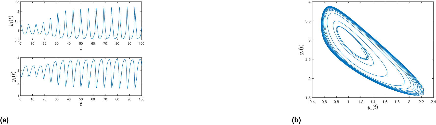
Example 3
Brusselator system with nonlinear
where
In this example, we cannot know the exact solution of (40). Therefore, we choose the value of
For the case of
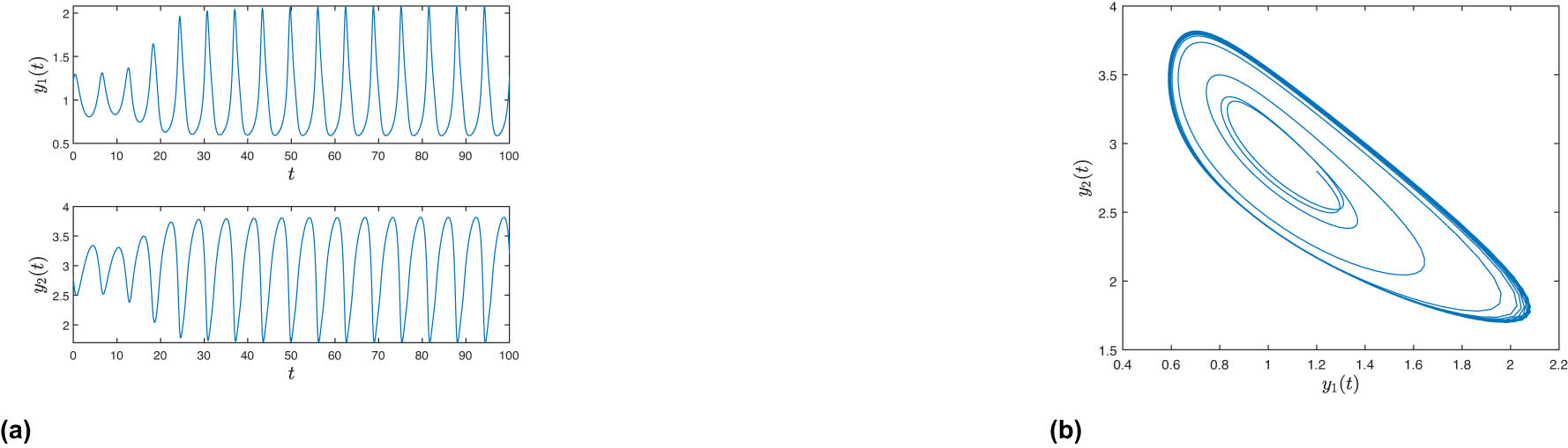
Behavior of the numerical solution for the system (40) with
Behavior of the numerical solution for the system (40) with
In this case, we find that the behavior of Figure 1 is in agreement with the work of Garrappa [27].
For the case of
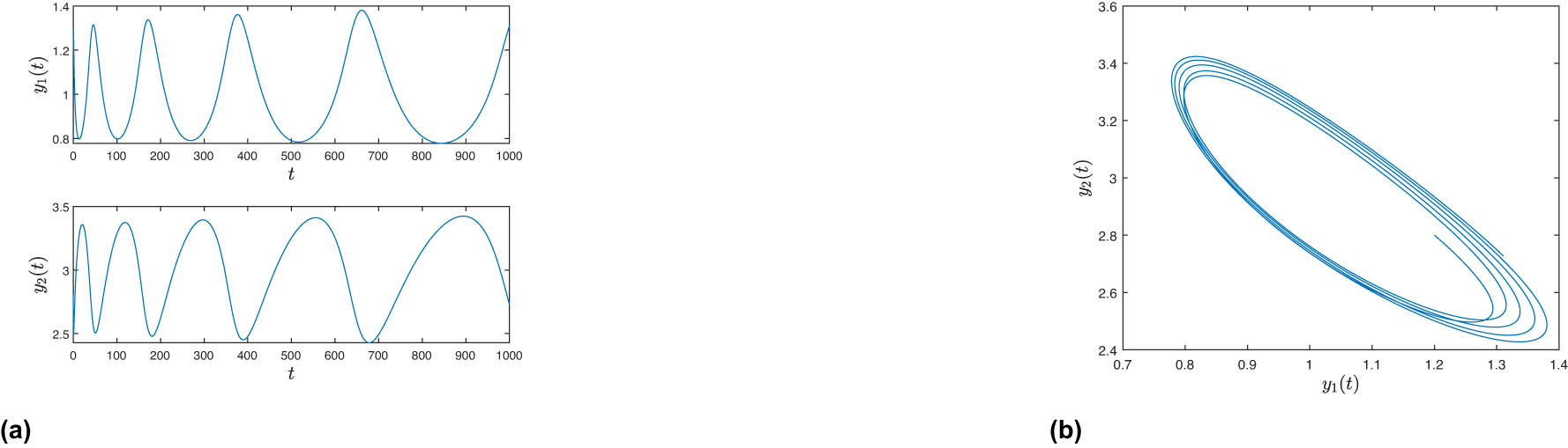
Behavior of the numerical solution for the system (40) with
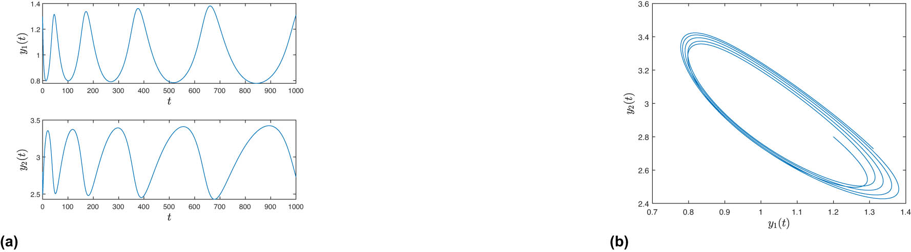
Behavior of the numerical solution for the system (40) with
6 Discussion and conclusion
In order to solve the nonlinear
Acknowledgement
The authors would like to thank the referees for their comments and suggestions which helped in improving the quality of the manuscript.
-
Funding information: This research project was supported by Thailand Science Research and Innovation (TSRI) Basic Research Fund: Fiscal year 2023 under project number FRB660073/0164.
-
Author contributions: The main idea of this work was proposed and mainly proved by P.S.N, while D.S. performed some proofs and provided some examples. All authors read and approved the final manuscript.
-
Conflict of interest: The authors state no conflict of interest.
References
[1] H. Sun, Y. Zhang, D. Baleanu, W. Chen, and Y. Chen, A new collection of real world applications of fractional calculus in science and engineering, Commun. Nonlinear Sci. Numer. Simul. 64 (2018), 213–231. 10.1016/j.cnsns.2018.04.019Search in Google Scholar
[2] P. Yi-Fei, Fractional differential analysis for texture of digital image, J. Algorithms Comput. Technol. 1 (2007), no. 3, 357–380. 10.1260/174830107782424075Search in Google Scholar
[3] C. M. Pinto and A. R. Carvalho, The HIV/TB coinfection severity in the presence of TB multi-drug resistant strains, Ecol. Complex. 32 (2017), 1–20. 10.1016/j.ecocom.2017.08.001Search in Google Scholar
[4] W. Chen, J. Zhang, and J. Zhang, A variable-order time-fractional derivative model for chloride ions sub-diffusion in concrete structures, Fract. Calc. Appl. Anal. 16 (2013), no. 1, 76–92. 10.2478/s13540-013-0006-ySearch in Google Scholar
[5] V. V. Tarasova and V. E. Tarasov, Concept of dynamic memory in economics, Commun. Nonlinear Sci. Numer. Simul. 55 (2018), 127–145. 10.1016/j.cnsns.2017.06.032Search in Google Scholar
[6] R. Garrappa, F. Mainardi, and M. Guido, Models of dielectric relaxation based on completely monotone functions, Fract. Calc. Appl. Anal. 19 (2016), no. 5, 1105–1160. 10.1515/fca-2016-0060Search in Google Scholar
[7] F. Jarad, T. Abdeljawad, and D. Baleanu, Caputo-type modification of the Hadamard fractional derivatives, Adv. Differential Equations 1 (2012), 1–8. 10.1186/1687-1847-2012-142Search in Google Scholar
[8] A. A. Kilbas, Hari M. Srivastava, and J. J. Trujillo, Theory and Applications of Fractional Differential Equations, North-Holland Mathematics Studies, Vol. 204, Elsevier Science Inc., New York, 2006. Search in Google Scholar
[9] Y. Luchko and J. Trujillo, Caputo-type modification of the Erdélyi-Kober fractional derivative, Fract. Calc. Appl. Anal. 10 (2007), no. 3, 249–267. Search in Google Scholar
[10] S. G. Samko, A. A. Kilbas, and O. I. Marichev, Fractional Integrals and Derivatives, Gordon and Breach Science Publishers, Amsterdam, 1993. Search in Google Scholar
[11] R. Almeida, A Caputo fractional derivative of a function with respect to another function, Commun. Nonlinear Sci. Numer. Simul. 44 (2017)460–481. 10.1016/j.cnsns.2016.09.006Search in Google Scholar
[12] R. Almeida, A. B. Malinowska, and M. T. T. Monteiro, Fractional differential equations with a Caputo derivative with respect to a kernel function and their applications, Math. Methods Appl. Sci. 41 (2018), no. 1, 336–352. 10.1002/mma.4617Search in Google Scholar
[13] R. Almeida, M. Jleli, and B. Samet, A numerical study of fractional relaxation-oscillation equations involving ψ-Caputo fractional derivative, Rev. R. Acad. Cienc. Exactas Fís. Nat. Ser. A Mat. RACSAM 113 (2019), no. 3, 1873–1891. 10.1007/s13398-018-0590-0Search in Google Scholar
[14] C. Derbazi, Z. Baitiche, M. Benchohra, and A. Cabada, Initial value problem for nonlinear fractional differential equations with ψ-Caputo derivative via monotone iterative technique, Axioms 9 (2020), no. 2, 57. 10.3390/axioms9020057Search in Google Scholar
[15] A. Suechoei and P. S. Ngiamsunthorn, Extremal solutions of φ-Caputo fractional evolution equations involving integral kernels, AIMS Math. 6 (2021), no. 5, 4734–4757. 10.3934/math.2021278Search in Google Scholar
[16] R. Almeida, A. B. Malinowska, and T. Odzijewicz, On systems of fractional differential equations with the ψ-Caputo derivative and their applications, Math. Methods Appl. Sci. 44 (2021), no. 10, 8026–8041. 10.1002/mma.5678Search in Google Scholar
[17] M. A. Zaitri, H. Zitane, and D. F. Torres, Pharmacokinetic/Pharmacodynamic anesthesia model incorporating psi-Caputo fractional derivatives, Comput. Biol. Med. 167 (2023), 107679. 10.1016/j.compbiomed.2023.107679Search in Google Scholar PubMed
[18] K. Diethelm, N. J. Ford, and A. D. Freed, A predictor–corrector approach for the numerical solution of fractional differential equations, Nonlinear Dyn. 29 (2002), no. 1, 3–22. 10.1023/A:1016592219341Search in Google Scholar
[19] C. Li and F. Zeng, The finite difference methods for fractional ordinary differential equations, Numer. Funct. Anal. Optim. 34 (2013), no. 2, 149–179. 10.1080/01630563.2012.706673Search in Google Scholar
[20] K. Pal, F. Liu, and Y. Yan, Numerical solutions of fractional differential equations by extrapolation, in: I. Dimov, I. Faragó, L. Vulkov (Eds.), Finite Difference Methods, Theory and Applications, FDM 2014, Lecture Notes in Computer Science, vol. 9045, Springer, Cham, 2014, pp. 299–306. 10.1007/978-3-319-20239-6_32Search in Google Scholar
[21] W. Qiu, O. Nikan, and Z. Avazzadeh, Numerical investigation of generalized tempered-type integro-differential equations with respect to another function, Fract. Calc. Appl. Anal. 26 (2023), no. 6, 2580–2601. 10.1007/s13540-023-00198-5Search in Google Scholar
[22] Y. Liu, J. Roberts, and Y. Yan, Detailed error analysis for a fractional Adams method with graded meshes, Numer. Algorithms 78 (2018), no. 4, 1195–1216. 10.1007/s11075-017-0419-5Search in Google Scholar
[23] D. Songsanga and P. S. Ngiamsunthorn, Single-step and multi-step methods for Caputo fractional-order differential equations with arbitrary kernels, AIMS Math. 7 (2022), no. 8, 15002–15028. 10.3934/math.2022822Search in Google Scholar
[24] K. Diethelm, Smoothness properties of solutions of Caputo-type fractional differential equations, Fract. Calc. Appl. Anal. 10 (2007), no. 2, 151–160. Search in Google Scholar
[25] C. W. H. Green, Y. Liu, and Y. Yan, Numerical methods for Caputo-Hadamard fractional differential equations with graded and non-uniform meshes, Mathematics 9 (2021), no. 21, 2728. 10.3390/math9212728Search in Google Scholar
[26] M. Stynes, E. O’Riordan, and J. L. Gracia, Error analysis of a finite difference method on graded meshes for a time-fractional diffusion equation, SIAM J. Numer. Anal. 55 (2017), no. 2, 1057–1079. 10.1137/16M1082329Search in Google Scholar
[27] R. Garrappa, Numerical solution of fractional differential equations: A survey and a software tutorial, Mathematics 6 (2018), no. 2, 16. 10.3390/math6020016Search in Google Scholar
© 2025 the author(s), published by De Gruyter
This work is licensed under the Creative Commons Attribution 4.0 International License.
Articles in the same Issue
- On I-convergence of nets of functions in fuzzy metric spaces
- Special Issue on Contemporary Developments in Graphs Defined on Algebraic Structures
- Forbidden subgraphs of TI-power graphs of finite groups
- Finite group with some c#-normal and S-quasinormally embedded subgroups
- Classifying cubic symmetric graphs of order 88p and 88p 2
- Two-sided zero-divisor graphs of orientation-preserving and order-decreasing transformation semigroups
- Simplicial complexes defined on groups
- Further results on permanents of Laplacian matrices of trees
- Algebra
- Classes of modules closed under projective covers
- On the dimension of the algebraic sum of subspaces
- Green's graphs of a semigroup
- On an uncertainty principle for small index subgroups of finite fields
- On a generalization of I-regularity
- Algorithm and linear convergence of the H-spectral radius of weakly irreducible quasi-positive tensors
- The hyperbolic CS decomposition of tensors based on the C-product
- On weakly classical 1-absorbing prime submodules
- Equational characterizations for some subclasses of domains
- Algebraic Geometry
- Spin(8, ℂ)-Higgs bundles fixed points through spectral data
- Embedding of lattices and K3-covers of an Enriques surface
- Kodaira-Spencer maps for elliptic orbispheres as isomorphisms of Frobenius algebras
- Applications in Computer and Information Sciences
- Dynamics of particulate emissions in the presence of autonomous vehicles
- Exploring homotopy with hyperspherical tracking to find complex roots with application to electrical circuits
- Category Theory
- The higher mapping cone axiom
- Combinatorics and Graph Theory
- 𝕮-inverse of graphs and mixed graphs
- On the spectral radius and energy of the degree distance matrix of a connected graph
- Some new bounds on resolvent energy of a graph
- Coloring the vertices of a graph with mutual-visibility property
- Ring graph induced by a ring endomorphism
- A note on the edge general position number of cactus graphs
- Complex Analysis
- Some results on value distribution concerning Hayman's alternative
- Freely quasiconformal and locally weakly quasisymmetric mappings in metric spaces
- A new result for entire functions and their shifts with two shared values
- On a subclass of multivalent functions defined by generalized multiplier transformation
- Singular direction of meromorphic functions with finite logarithmic order
- Growth theorems and coefficient bounds for g-starlike mappings of complex order λ
- Refinements of inequalities on extremal problems of polynomials
- Control Theory and Optimization
- Averaging method in optimal control problems for integro-differential equations
- On superstability of derivations in Banach algebras
- The robust isolated calmness of spectral norm regularized convex matrix optimization problems
- Observability on the classes of non-nilpotent solvable three-dimensional Lie groups
- Differential Equations
- The ill-posedness of the (non-)periodic traveling wave solution for the deformed continuous Heisenberg spin equation
- A note on the global existence and boundedness of an N-dimensional parabolic-elliptic predator-prey system with indirect pursuit-evasion interaction
- Blow-up of solutions for Euler-Bernoulli equation with nonlinear time delay
- Periodic or homoclinic orbit bifurcated from a heteroclinic loop for high-dimensional systems
- Regularity of weak solutions to the 3D stationary tropical climate model
- Local minimizers for the NLS equation with localized nonlinearity on noncompact metric graphs
- Global existence and blow-up of solutions to pseudo-parabolic equation for Baouendi-Grushin operator
- Bubbles clustered inside for almost-critical problems
- Existence and multiplicity of positive solutions for multiparameter periodic systems
- Existence of positive periodic solutions for evolution equations with delay in ordered Banach spaces
- On a nonlinear boundary value problems with impulse action
- Normalized ground-states for the Sobolev critical Kirchhoff equation with at least mass critical growth
- Multiple positive solutions to a p-Kirchhoff equation with logarithmic terms and concave terms
- Infinitely many solutions for a class of Kirchhoff-type equations
- Real and non-real eigenvalues of regular indefinite Sturm–Liouville problems
- Existence of global solutions to a semilinear thermoelastic system in three dimensions
- Limiting profile of positive solutions to heterogeneous elliptic BVPs with nonlinear flux decaying to negative infinity on a portion of the boundary
- Morse index of circular solutions for repulsive central force problems on surfaces
- Differential Geometry
- On tangent bundles of Walker four-manifolds
- Pedal and negative pedal surfaces of framed curves in the Euclidean 3-space
- Discrete Mathematics
- Eventually monotonic solutions of the generalized Fibonacci equations
- Dynamical Systems Ergodic Theory
- Dynamical properties of two-diffusion SIR epidemic model with Markovian switching
- A note on weighted measure-theoretic pressure
- Pullback attractors for a class of second-order delay evolution equations with dispersive and dissipative terms on unbounded domain
- Pullback attractor of the 2D non-autonomous magneto-micropolar fluid equations
- Functional Analysis
- Spectrum boundary domination of semiregularities in Banach algebras
- Approximate multi-Cauchy mappings on certain groupoids
- Investigating the modified UO-iteration process in Banach spaces by a digraph
- Tilings, sub-tilings, and spectral sets on p-adic space
- Continuity and essential norm of operators defined by infinite tridiagonal matrices in weighted Orlicz and l∞ spaces
-
A family of commuting contraction semigroups on
- q-Stirling sequence spaces associated with q-Bell numbers
- Chlodowsky variant of Bernstein-type operators on the domain
- Hyponormality on a weighted Bergman space of an annulus with a general harmonic symbol
- Characterization of derivations on strongly double triangle subspace lattice algebras by local actions
- Fixed point approaches to the stability of Jensen’s functional equation
- Geometry
- The regularity of solutions to the Lp Gauss image problem
- Solving the quartic by conics
- Group Theory
- On a question of permutation groups acting on the power set
- A characterization of the translational hull of a weakly type B semigroup with E-properties
- Harmonic Analysis
- Eigenfunctions on an infinite Schrödinger network
- Maximal function and generalized fractional integral operators on the weighted Orlicz-Lorentz-Morrey spaces
- Subharmonic functions and associated measures in ℝn
- Mathematical Logic, Model Theory and Foundation
- A topology related to implication and upsets on a bounded BCK-algebra
- Boundedness of fractional sublinear operators on weighted grand Herz-Morrey spaces with variable exponents
- Number Theory
- Fibonacci vector and matrix p-norms
- Recurrence for probabilistic extension of Dowling polynomials
- Carmichael numbers composed of Piatetski-Shapiro primes in Beatty sequences
- The number of rational points of some classes of algebraic varieties over finite fields
- Classification and irreducibility of a class of integer polynomials
- Decompositions of the extended Selberg class functions
- Joint approximation of analytic functions by the shifts of Hurwitz zeta-functions in short intervals
- Fibonacci Cartan and Lucas Cartan numbers
- Recurrence relations satisfied by some arithmetic groups
- The hybrid power mean involving the Kloosterman sums and Dedekind sums
- Numerical Methods
- A modified predictor–corrector scheme with graded mesh for numerical solutions of nonlinear Ψ-caputo fractional-order systems
- A kind of univariate improved Shepard-Euler operators
- Probability and Statistics
- Statistical inference and data analysis of the record-based transmuted Burr X model
- Multiple G-Stratonovich integral in G-expectation space
- p-variation and Chung's LIL of sub-bifractional Brownian motion and applications
- Real Analysis
- Chebyshev polynomials of the first kind and the univariate Lommel function: Integral representations
- Multiple solutions for a class of fourth-order elliptic equations with critical growth
- Majorization-type inequalities for (m, M, ψ)-convex functions with applications
- The evaluation of a definite integral by the method of brackets illustrating its flexibility
- Some new Fejér type inequalities for (h, g; α - m)-convex functions
- Some new Hermite-Hadamard type inequalities for product of strongly h-convex functions on ellipsoids and balls
- Topology
- Unraveling chaos: A topological analysis of simplicial homology groups and their foldings
- A generalized fixed-point theorem for set-valued mappings in b-metric spaces
- On SI2-convergence in T0-spaces
- Generalized quandle polynomials and their applications to stuquandles, stuck links, and RNA folding