The hyperbolic CS decomposition of tensors based on the C-product
-
Hongwei Jin
 ,
Siran Chen
,
Siran Chen

Abstract
This paper studies the issues about the hyperbolic CS decomposition of tensors under the C-product. The aim of this paper is fourfold. Firstly, we establish the CS decomposition of a complex unitary tensor, including the thin version and the standard version. The corresponding numerical algorithm is also given. Next, we define three kinds of tensors, i.e., the strong unitary tensor, the mode-1 strong unitary tensor, the mode-2 strong unitary tensor, and we give the CS decomposition of the last two kind of tensors aforementioned. Numerical algorithms are also obtained to compute the two types of the CS decompositions. Moreover, we give the definition of another three classes of tensors, called the
1 Introduction
In recent years, the researches of tensors or multidimensional arrays have become more popular. A complex tensor can be regarded as a multidimensional array of data, which takes the form
Higher-order tensors have been applied in quite a lot of areas, such as psychometrics [1], chemometrics [2], face recognition [3], image and signal processing [4], [5], [6], [7], [8], [9] and so on.
The tensor decomposition has developed very well and found to have good applications in many fields, such as in eigenvalues, genomic signals, data mining, signal processing [10], [11], [12], [13], [14], [15], [16]. Kinds of tensor decompositions via diverse tensor products have been investigated to extend the matrices contents. For example, [17], [18], [19], [20], [21].
The tensor-tensor products include the Einstein product, T-product, C-product and so on. Lots of excellent works had appeared, such as: Sun et al. [22],23] studied the issue about the generalized inverse of tensors based on the Einstein product and a general product of tensors. Miao et al. [24], [25], [26] studied the tensor contents under the T-product. Panigrahy et al. [27] and Behera et al. [28] studied the reverse order law and computation concerning the Einstein product and T-product. Liu et al. [29] studied the issue of the dual core generalized inverse. Cong et al. [30] and Sahoo et al. [31] studied the core-EP inverse of tensors. Jin et al. [32] researched some work on the generalized inverse of tensors based on the T-product. Behera et al. [33],34] and Ji et al. [35] got some results on the Drazin inverse of the Einstein product. Cao et al. [36],37] had a further study on the perturbation and inequalities based on the T-product. Che et al. [38] established an efficient algorithm for computing the approximate t-URV. Chen et al. [39] studied the perturbations of the tensor Schur decomposition and Liu et al. [40] studied the weighted generalized tensor functions. Mo et al. [41],42] studied on the Time-varying generalized tensor eigenanalysis and T-eigenvalues of tensors. Wei et al. [43] studied the Neural network models and Shao et al. [44] studied the nonsymmetric algebraic Riccati equations.
Kernfeld et al. [45] defined a new tensor-tensor product, that is, the Cosine Transform Product, referred to as C-product for short. It has been shown that the C-product can be implemented efficiently using DCT (Discrete Cosine Transform). Moreover, the authors indicated that one can use C-product to conveniently specify a discrete image blurring model and the image restoration model. Bentbib et al. [46] explored good applications of the C-product. They proposed new methods for the problem of the third-order tensor completion in combination with the TV regularization procedure and tensor robust principal component analysis by using the C-product. Xu et al. [47] indicated that the advantages of using DCT are: (1) the complex calculation is not involved in the cosine transform based singular value decomposition, so the computational costs can be saved; (2) the intrinsic reflexive boundary condition along the tubes in the third dimension of tensors is employed, so its performance would be better than that by using the periodic boundary condition in DFT (Discrete Fourier Transform).
The CS decomposition is a very useful tool in the matrix analysis. Benítez et al. [48] studied the spectrum and the rank of a linear combination of two orthogonal projectors. By using the CS decomposition, the authors characterized when this linear combination is EP, diagonalizable, idempotent, tripotent, involutive, nilpotent, generalized projector, and hypergeneralized projector. The Moore-Penrose inverse of a linear combination of two orthogonal projectors in a special case was also derived. Calvetti et al. [49] indicated that the Schur form of the real orthogonal matrix can be got from a full CS decomposition. Based on this fact, the authors derived a CS decomposition based on the orthogonal eigenvalue method. An algorithm for an orthogonal similarity transformation of an orthogonal matrix to a condensed product form and an algorithm for full CS decomposition were also described.
Based on these backgrounds, we will study the theory of the hyperbolic CS decomposition of tensors via the C-product in this paper.
This paper is organized as follows. In Section 2, we give the terms and symbols needed to be used in this work. Then, we introduce the C-product of two tensors. In Section 3, we firstly introduce the thin version of the CS decomposition of a complex unitary tensor. Then, a standard CS decomposition of a complex unitary tensor is obtained. In Section 3, we define three kinds of tensors, i.e., the strong unitary tensor, the mode-1 strong unitary tensor and the mode-2 strong unitary tensor. Then, the CS decomposition and corresponding numerical algorithms of the mode-1 strong unitary tensor and the mode-2 strong unitary tensor are constructed. In the next section, we define another three classes of tensors, i.e., the
2 Preliminaries
In this paper, we denote vectors, matrices, three or higher order tensors like
We start this section by introducing the following face-wise product between two tensors.
Definition 1.
[45] Let
The following example is helpful in understanding this product.
Example 1.
Let
Then,
□
Now, we will present the C-product of two tensors. Firstly, we give the definition of the operation of mat(⋅).
Definition 2.
[45] Let
where O is the n 1 × n 2 zero matrix.
Definition 3.
[45] Define ten(⋅) the inverse operation of the mat(⋅), i.e.,
Now, we can give the C-product of two tensors.
Definition 4.
[45] Let
From the above definition, we can see that it is easy to compute
| Algorithm 2.1: Compute ten(⋅) of a matrix |
| Input: n 1 n 3 × n 2 n 3 block matrix Z |
|
Output: n
1 × n
2 × n
3 tensor
|
| 1. Take the bottom left n
1 × n
2 block of Z and
|
| 2. for i = n 3 − 1, …, 1 |
|
|
| end |
Notice that the first column of
So, it is easy to get all the frontal slices of
Now, we present another way to define the C-product of two tensors by using the face-wise product. Before that, the mode-3 product of a tensor with a matrix is required.
Definition 5.
[20] The mode-3 product of a tensor
Now, we will introduce how to compute the mode-3 product of a tensor with a matrix. Let the frontal slice of
Then, the mode-3 unfolding of
Notice that
The following example shows how to compute the mode-3 product of a tensor with a matrix.
Example 2.
Let
Suppose
Hence,
Thus,
□
Based on the above preparation work, we can get the alternative expression of the C-product. Observe that
Lemma 1.
[45] Let
where M = W
−1
C(I + Z), W = diag(C(:, 1)), C(:, 1) is the first column of C, the matrix
C is the orthogonal DCT matrix of size n 3 × n 3 and its elements are defined as
δ ij is the Kronecker symbol.
Now, we give an example to show the details to implement the C-product.
Example 3.
Let
In this case, M is a 2 × 2 matrix and can be computed by using the Matlab. More precisely, M and M −1 are
By (4), we can compute
Then, we can get
By the last step, we can get the C-product of
□
An algorithm of the C-product of
| Algorithm 2.2: Compute the C-product of two tensors [45] |
|
Input: n
1 × n
2 × n
3 tensor
|
|
Output: n
1 × l × n
3 tensor
|
| 1. Compute M = W −1 C(I + Z) as in Lemma 1 |
| 2. Compute
|
| 3. for i = 1, …, n 3 |
|
|
| end |
| 4.
|
By Algorithm 2.2, we can get the following lemma.
Lemma 2.
Let
Let
Lemma 3.
[45] Let
where ⊗ is the Kronecker product and
Definition 6.
[45] Let
Definition 7.
[45] Let
then
We can check that the inverse of a tensor, if exists, is unique. The conjugate transpose of tensors can be defined as follows.
Definition 8.
[45] If
Lemma 4.
[45] Let
Definition 9.
[45] The tensor
Definition 10.
[50] Let
The following lemma is helpful in establishing the main result of next sections.
Lemma 5.
[50] Let
The next lemma explains the operation of two block tensors.
Lemma 6.
[51] Let
In the following, we show that the L(⋅) operation of the block tensor has the good character.
Lemma 7.
Let
Proof.
Let
Hence, we claim that
□
3 The CS decomposition of the unitary tensor
In this section, we will study the CS decomposition of the unitary tensor based on C-product. Firstly, we give a thin version of the CS decomposition of the unitary tensor.
Theorem 1.
Let
be a partially unitary tensor. Then, there exist unitary tensors
where
Proof.
Since
Hence,
by using Lemma 7, we have
Now, we can get the CS decomposition of
where
with
By Definition 1 and using (9) and (10), we have
with
Implementing the operation “L −1(⋅)” on both sides of the equalities (11) and (12), we have
with
Since
In the following, we will establish a more general version of the CS decomposition of tensors.
Theorem 2.
Let
be a unitary tensor. Then, there exist unitary tensors
where
Proof.
Since
which implies that
by Lemma 7, we get
By using the CS decomposition [53] of
where
with
By Definition 1, we have
with
Utilizing the operation “L −1(⋅)” on both sides of the equalities (17) and (18), we have
with
By Lemma 5, we get
In the following, we will build an efficient algorithm to compute the CS decomposition of a unitary tensor by Theorem 2.
| Algorithm 3.1: Compute the CS decomposition of a unitary tensor |
|
Input: (m
1 + m
2) × (m
1 + m
2) × p unitary tensor
|
|
Output:
|
| 1. Compute
|
| 2. for i = 1, …, p |
|
|
| end |
| 3.
|
Example 4.
Let
A simple computation gives
The first step, we will compute the singular value decomposition of
Then,
Similarly, by computing the singular value decomposition of
Hence, there exist orthogonal tensors
and
Then,
and
Finally, one can check that
4 The CS decomposition of a strong unitary tensor
In this section, we will study the CS decomposition of a strong unitary tensor. Firstly, let us give the definition of a related tensor.
Definition 11.
Let
where
Two more general versions of the strong unitary tensor is given as follows.
Definition 12.
Let
where
where
Now, we will do some researches on the CS decomposition of the mode-1 (mode-2) strong unitary tensor.
Theorem 3.
Let
be a mode-1 strong unitary tensor. Then, there exist a mode-1 strong unitary tensors
where
Proof.
Since
Let
where
Hence,

Let
Theorem 4.
Let
be a mode-2 strong unitary tensor. Then, there exist unitary tensors
where
Proof.
The proof is similar as Theorem 3. □
In the following, we will give an algorithm to compute the CS decomposition of a mode-1 strong unitary tensor.
| Algorithm 4.1: Compute the CS decomposition of a mode-1 strong unitary tensor |
|
Input: (m
1 + m
2) × (m
1 + m
2) × p mode-1 strong unitary
|
|
Output:
|
| 1. Compute
|
| 2. Construct an F-diagonal tensor
|
| 3. Compute
|
| 4. Compute
|
| 5. for i = 1, …, p |
|
|
| end |
| 6.
|
| 7.
|
Example 5.
Let
A simple computation gives
Then,
which means
Then,
Moreover,
Next, it is easy to execute Algorithm 3.1 to get the CS decomposition of the mode-1 strong unitary tensor. □
Similar as Algorithm 4.1, we can get an algorithm to compute the CS decomposition of a mode-2 strong unitary tensor.
5 The hyperbolic CS decomposition of tensors
In this section, we firstly give some definitions of the
Definition 13.
[54] Let
where
Definition 14.
Let
where
then
The definition of a
Definition 15.
Let
where
where
Moreover, the definition of the strong
Definition 16.
Let
where
where
Definition 17.
Let
where
where
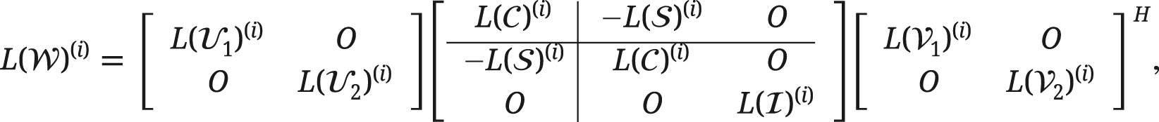
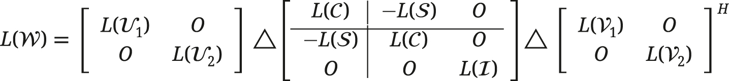
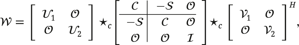
The following result is the hyperbolic CS decomposition of a
Theorem 5.
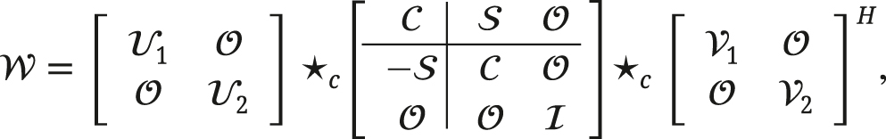
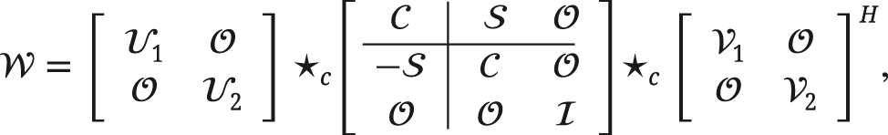
Let
be a
where
Proof.
Since
which means
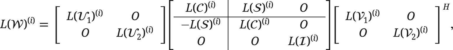
by Lemma 7, we get
Using Theorem 3.2 of [54], we have
where
with
By Definition 1, we have
with
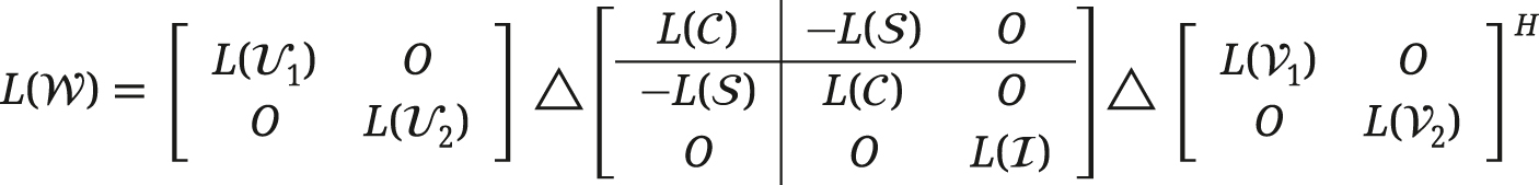
Implementing the operation “L −1(⋅)” on both sides of the equalities (23) and (24), we have
with
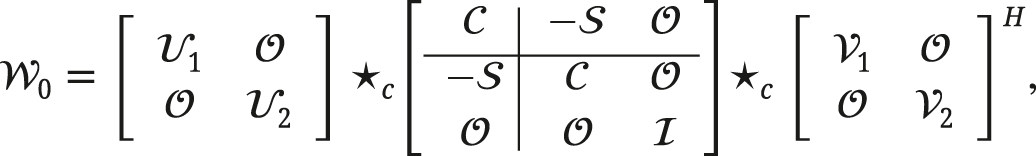
Similar as Theorem 1, we get that
Let
If
It is easy to check
Now, we can set up an algorithm for the hyperbolic CS decomposition of the
|
Algorithm 5.1: Compute the hyperbolic CS decomposition of a
|
|
Input:
|
|
Output:
|
| 1. Compute
|
| 2. Compute
|
| 3. for i = 1, …, p |
|
|
| end |
| 4.
|
| 5.
|
Example 6.
Let
A simple computation gives
By using the formula
where
It is easy to check that
In the last step, we compute
Therefore,
Hence,
□
In the following, we give the hyperbolic CS decomposition of a mode-1 strong
Theorem 6.
Let
be a mode-1 strong

where
Proof.
Since
Define
Then, we have
Let
where
Therefore,
Let
Similar as Theorem 6, we can get the hyperbolic CS decomposition of a mode-2 strong
Theorem 7.
Let
be a mode-2 strong

where
In the following, we will give an algorithm to compute the hyperbolic CS decomposition of the mode-1 strong
|
Algorithm 5.2: Compute the hyperbolic CS decomposition of the mode-1 strong
|
|
Input:
|
|
Output:
|
| 1. Compute
|
| 2. Construct an F-diagonal tensor
|
| 3. Compute
|
| 4. Compute
|
| 5. Compute
|
| 6. for i = 1, …, p |
|
|
| end |
| 7.
|
| 8.
|
| 9.
|
6 An application to the computation of the C-eigenvalues of a tensor
Firstly, we will introduce the C-eigenvalue of the tensor
Definition 18.
Let
then λ is called a C-eigenvalue of
Notice that
The following theorem involves a full CS decomposition of a unitary tensor.
Theorem 8.
Let
be a unitary tensor. Then, there exist unitary tensors
where
The next lemma is helpful in establish the main result.
Lemma 8.
Let
where
Proof.
Since
Thus,
which implies
Define
Then, we have
and
Using (31), one has there exists an orthogonal tensor
where
and
Similar, using (32), one has that there exists an orthogonal tensor
where
and
Let I
n
be the n × n identity matrix and e
j
be the jth column of I
n
. Denote the tensor
and
Then, one has
Define
By using
one has
Since
where
with
one has
where
Let
Therefore, one can compute the eigenvalues of
Example 7.
Let
A simple computation gives
Then, the full CS decompositions of
Then,
By computing the eigenvalues of
one can get the C-eigenvalues of the orthogonal tensor
Acknowledgments
The authors would like to thank the anonymous reviewers for their valuable comments, which have significantly improved the paper.
-
Research ethics: Not applicable.
-
Informed consent: Not applicable.
-
Author contributions: All authors have accepted responsibility for the entire content of this manuscript and consented to its submission to the journal, reviewed all the results, and approved the final version of the manuscript. All authors contributed equally to the manuscript.
-
Use of Large Language Models, AI and Machine Learning Tools: None declared.
-
Conflict of interest: The authors state no conflicts of interest.
-
Research funding: This work was supported by the Special Fund for Science and Technological Bases and Talents of Guangxi (No. GUIKE AA24010005).
-
Data availability: Some or all data, models, or code generated or used during the study are available from the corresponding author by request.
References
[1] P. Kroonenberg, Three-Mode Principal Component Analysis: Theory and Applications, DSWO Press, Leiden, 1983.Search in Google Scholar
[2] M. Ng, R. Chan, and W. Tang, A fast algorithm for deblurring models with Neumann boundary conditions, SIAM J. Sci. Comput. 21 (1999), no. 3, 851–866, https://doi.org/10.1137/S1064827598341384.Search in Google Scholar
[3] N. Hao, M. Kilmer, K. Braman, and R. Hoover, Facial recognition using tensor-tensor decompositions, SIAM J. Imaging Sci. 6 (2013), no. 1, 437–463, https://doi.org/10.1137/110842570.Search in Google Scholar
[4] P. Comon, Tensor decompositions: state of the art and applications, Proceedings of the Institute of Mathematics and its Applications Conference Series, Institute of Mathematics and its Applications, Oxford, 2002, pp. 1–28.10.1093/oso/9780198507345.003.0001Search in Google Scholar
[5] L. De Lathauwer and B. De Moor, From matrix to tensor: Multilinear algebra and signal processing, in: J. McWhirter and I. K. Proudler (eds), Mathematics in Signal Processing IV, Clarendon Press, Oxford, UK, 1998, pp. 1–15.Search in Google Scholar
[6] J. Nagy and M. Kilmer, Kronecker product approximation for preconditioning in three-dimensional imaging applications, IEEE Trans. Image Process. 15 (2006), no. 3, 604–613, https://doi.org/10.1109/TIP.2005.863112.Search in Google Scholar PubMed
[7] N. Sidiropoulos, R. Bro, and G. Giannakis, Parallel factor analysis in sensor array processing, IEEE Trans. Signal Process. 48 (2000), no. 8, 2377–2388, https://doi.org/10.1109/78.852018.Search in Google Scholar
[8] W. Hoge and C. Westin, Identification of translational displacements between N-dimensional data sets using the high order SVD and phase correlation, IEEE Trans. Image Process. 14 (2005), no. 7, 884–889, https://doi.org/10.1109/TIP.2005.849327.Search in Google Scholar
[9] M. Rezghi and L. Eldén, Diagonalization of tensors with circulant structure, Linear Algebra Appl. 435 (2011), no. 3, 422–447, https://doi.org/10.1016/j.laa.2010.03.032.Search in Google Scholar
[10] M. Che, L. Qi, and Y. Wei, The generalized order tensor complementarity problems, Numer. Math. Theor. Meth. Appl. 13 (2020), no. 1, 131–149, https://doi.org/10.4208/nmtma.OA-2018-0117.Search in Google Scholar
[11] A. Cichocki, R. Zdunek, A. H. Phan, and S. I. Amari, Nonnegative Matrix and Tensor Factorizations: Applications to Exploratory Multi-Way Data Analysis and Blind Source Separation, John Wiley and Sons, Hoboken, 2009.10.1002/9780470747278Search in Google Scholar
[12] L. De Lathauwer, Signal Processing Based on Multilinear Algebra, PhD Thesis, Katholike Universiteit, Leuven, 1997.Search in Google Scholar
[13] Y. Miao, L. Qi, and Y. Wei, M-eigenvalues of the Riemann curvature tensor of conformally flat manifolds, 2018, arXiv:1808.01882, https://doi.org/10.48550/arXiv.1808.01882.Search in Google Scholar
[14] L. Omberg, G. H. Golub, and O. Alter, A tensor higher-order singular value decomposition for integrative analysis of DNA microarray data from different studies, Proc. Natl. Acad. Sci. USA 104 (2007), no. 47, 18371–18376, https://doi.org/10.1073/pnas.0709146104.Search in Google Scholar PubMed PubMed Central
[15] L. Xiong and J. Liu, A new C-eigenvalue localisation set for piezoelectric-type tensors, East Asian J. Appl. Math. 10 (2020), no. 1, 123–134, https://doi.org/10.4208/eajam.060119.040619.Search in Google Scholar
[16] X. Wang, M. Che, and Y. Wei, Best rank-one approximation of fourth-order partially symmetric tensors by neural network, Numer. Math. Theor. Meth. Appl. 11 (2018), no. 4, 673–700, https://doi.org/10.4208/nmtma.2018.s01.Search in Google Scholar
[17] J. D. Carroll and J. J. Chang, Analysis of individual differences in multidimensional scaling via an N-way generalization of “Eckart-Young” decomposition, Psychometrika 35 (1970), no. 3, 283–319, https://doi.org/10.1007/BF02310791.Search in Google Scholar
[18] L. De Lathauwer, B. De Moor, and J. Vandewalle, A multilinear singular value decomposition, SIAM J. Matrix Anal. Appl. 21 (2000), no. 4, 1253–1278, https://doi.org/10.1137/S0895479896305727.Search in Google Scholar
[19] Z. H. He, C. Chen, and X. X. Wang, A simultaneous decomposition for three quaternion tensors with applications in color video signal processing, Anal. Appl. 19 (2021), no. 3, 423–444, https://doi.org/10.1142/S0219530520400084.Search in Google Scholar
[20] T. G. Kolda and B. W. Bader, Tensor decompositions and applications, SIAM Rev. 51 (2009), no. 3, 455–500, https://doi.org/10.1137/07070111X.Search in Google Scholar
[21] L. Tucker, Some mathematical notes on three-mode factor analysis, Psychometrika 31 (1966), no. 3, 279–311, https://doi.org/10.1007/BF02289464.Search in Google Scholar PubMed
[22] L. Sun, B. Zheng, C. Bu, and Y. Wei, Moore-Penrose inverse of tensors via Einstein product, Linear Multilinear Algebra 64 (2016), no. 4, 686–698, https://doi.org/10.1080/03081087.2015.1083933.Search in Google Scholar
[23] L. Sun, B. Zheng, Y. Wei, and C. Bu, Generalized inverses of tensors via a general product of tensors, Front. Math. China 13 (2018), no. 4, 893–911, https://doi.org/10.1007/s11464-018-0695-y.Search in Google Scholar
[24] Y. Miao, L. Qi, and Y. Wei, Generalized tensor function via the tensor singular value decomposition based on the T-product, Linear Algebra Appl. 590 (2020), 258–303, https://doi.org/10.1016/j.laa.2019.12.035.Search in Google Scholar
[25] Y. Miao, L. Qi, and Y. Wei, T-Jordan canonical form and T-Drazin inverse based on the T-product, Commun. Appl. Math. Comput. 3 (2021), 201–220, https://doi.org/10.1007/s42967-019-00055-4.Search in Google Scholar
[26] Y. Miao, T. Wang, and Y. Wei, Stochastic conditioning of tensor functions based on the tensor-tensor product, Pac. J. Optim. 19 (2023), no. 2, 205–235, https://doi.org/10.1016/j.pjopt.2022.11.002.Search in Google Scholar
[27] K. Panigrahy, R. Behera, and D. Mishra, Reverse order law for the Moore-Penrose inverses of tensors, Linear Multilinear Algebra 68 (2020), no. 2, 246–264, https://doi.org/10.1080/03081087.2018.1502252.Search in Google Scholar
[28] R. Behera, J. Sahoo, R. Mohapatra, and M. Nashed, Computation of generalized inverses of tensors via T-product, Numer. Linear Algebra Appl. 29 (2021), no. 2, e2416, https://doi.org/10.1002/nla.2416.Search in Google Scholar
[29] Y. Liu and H. Ma, Dual core generalized inverse of third-order dual tensor based on the T-product, Comput. Appl. Math. 41 (2022), no. 8, 391, https://doi.org/10.1007/s40314-022-02114-8.Search in Google Scholar
[30] Z. Cong and H. Ma, Characterizations and perturbations of the core-EP inverse of tensors based on the T-product, Numer. Funct. Anal. Optim. 43 (2022), no. 10, 1150–1200, https://doi.org/10.1080/01630563.2022.2087676.Search in Google Scholar
[31] J. Sahoo, R. Behera, P. Stanimirović, V. Katsikis, and H. Ma, Core and core-EP inverses of tensors, Comput. Appl. Math. 39 (2020), no. 9, 9, https://doi.org/10.1007/s40314-019-0983-5.Search in Google Scholar
[32] H. Jin, M. Bai, J. Benítez, and X. Liu, The generalized inverses of tensors and an application to linear models, Comput. Math. Appl. 74 (2017), no. 3, 385–397, https://doi.org/10.1016/j.camwa.2017.04.017.Search in Google Scholar
[33] R. Behera and D. Mishra, Further results on generalized inverses of tensors via the Einstein product, Linear Multilinear Algebra 65 (2017), no. 8, 1662–1682, https://doi.org/10.1080/03081087.2016.1253662.Search in Google Scholar
[34] R. Behera, A. Nandi, and J. Sahoo, Further results on the Drazin inverse of even order tensors, Numer. Linear Algebra Appl. 27 (2020), no. 5, e2317, https://doi.org/10.1002/nla.2317.Search in Google Scholar
[35] J. Ji and Y. Wei, The Drazin inverse of an even-order tensor and its application to singular tensor equations, Comput. Math. Appl. 75 (2018), no. 9, 3402–3413, https://doi.org/10.1016/j.camwa.2018.02.006.Search in Google Scholar
[36] Z. Cao and P. Xie, Perturbation analysis for t-product-based tensor inverse, Moore-Penrose inverse and tensor system, Commun. Appl. Math. Comput. 4 (2022), no. 4, 1441–1456, https://doi.org/10.1007/s42967-022-00186-1.Search in Google Scholar
[37] Z. Cao and P. Xie, On some tensor inequalities based on the T-product, Linear Multilinear Algebra 71 (2023), no. 3, 377–390, https://doi.org/10.1080/03081087.2022.2032567.Search in Google Scholar
[38] M. Che and Y. Wei, An efficient algorithm for computing the approximate t-URV and its applications, J. Sci. Comput. 92 (2022), no. 3, 93, https://doi.org/10.1007/s10915-022-01956-y.Search in Google Scholar
[39] J. Chen, W. Ma, Y. Miao, and Y. Wei, Perturbations of Tensor-Schur decomposition and its applications to multilinear control systems and facial recognitions, Neurocomputing 547 (2023), 126359, https://doi.org/10.1016/j.neucom.2023.126359.Search in Google Scholar
[40] Y. Liu and H. Ma, Weighted generalized tensor functions based on the tensor-product and their applications, Filomat 36 (2022), no. 18, 6403–6426, https://doi.org/10.2298/fil2218403l.Search in Google Scholar
[41] C. Mo, X. Wang, and Y. Wei, Time-varying generalized tensor eigenanalysis via Zhang neural networks, Neurocomputing 407 (2020), 465–479, https://doi.org/10.1016/j.neucom.2020.04.115.Search in Google Scholar
[42] C. Mo, W. Ding, and Y. Wei, Perturbation analysis on T-eigenvalues of third-order tensors, J. Optim. Theor. Appl. 202 (2024), no. 2, 668–702, https://doi.org/10.1007/s10957-024-02444-z.Search in Google Scholar
[43] P. Wei, X. Wang, and Y. Wei, Neural network models for time-varying tensor complementarity problems, Neurocomputing 523 (2023), 18–32, https://doi.org/10.1016/j.neucom.2022.12.008.Search in Google Scholar
[44] X. Shao, Y. Wei, and J. Yuan, Nonsymmetric algebraic Riccati equations under the tensor product, Numer. Funct. Anal. Optim. 44 (2023), no. 6, 545–563, https://doi.org/10.1080/01630563.2023.2192593.Search in Google Scholar
[45] E. Kernfeld, M. Kilmer, and S. Aeron, Tensor-tensor products with invertible linear transforms, Linear Algebra Appl. 485 (2015), 545–570, https://doi.org/10.1016/j.laa.2015.07.021.Search in Google Scholar
[46] A. Bentbib, A. El Hachimi, K. Jbilou, and A. Ratnani, Fast multidimensional completion and principal component analysis methods via the cosine product, Calcolo 59 (2022), no. 3, 26, https://doi.org/10.1007/s10092-022-00469-2.Search in Google Scholar
[47] W. Xu, X. Zhao, and M. Ng, A fast algorithm for cosine transform based tensor singular value decomposition, 2019, arXiv:1902.03070, https://doi.org/10.48550/arXiv.1902.03070.Search in Google Scholar
[48] J. Benítez and V. Rakočević, Applications of CS decomposition in linear combinations of two orthogonal projectors, Appl. Math. Comput. 203 (2008), no. 2, 761–769, https://doi.org/10.1016/j.amc.2008.05.053.Search in Google Scholar
[49] D. Calvetti, L. Reichel, and H. Xu, A CS decomposition for orthogonal matrices with application to eigenvalue computation, Linear Algebra Appl. 476 (2015), 197–232, https://doi.org/10.1016/j.laa.2015.03.007.Search in Google Scholar
[50] H. Jin, S. Xu, H. Jiang, and X. Liu, The generalized inverses of tensors via the C-product, 2022, arXiv:2211.02841, https://doi.org/10.48550/arXiv.2211.02841.Search in Google Scholar
[51] H. Jin, M. He, and Y. Wang, The expressions of the generalized inverses of the block tensor via the C-product, Filomat 26 (2023), no. 37, 909–932, https://doi.org/10.2298/FIL2326909J.Search in Google Scholar
[52] G. H. Golub and C. F. Van Loan, Matrix Computations, 4th ed., Johns Hopkins Univ. Press, Baltimore, 2013.Search in Google Scholar
[53] S. Xu, Theory and Methods of Computation of Matrices, Peking University Press, Beijing, 1995.Search in Google Scholar
[54] N. J. Higham, J-orthogonal matrices: properties and generation, SIAM Rev. 45 (2003), no. 3, 504–519, https://doi.org/10.1137/S0036144502414930.Search in Google Scholar
© 2025 the author(s), published by De Gruyter, Berlin/Boston
This work is licensed under the Creative Commons Attribution 4.0 International License.
Articles in the same Issue
- On I-convergence of nets of functions in fuzzy metric spaces
- Special Issue on Contemporary Developments in Graphs Defined on Algebraic Structures
- Forbidden subgraphs of TI-power graphs of finite groups
- Finite group with some c#-normal and S-quasinormally embedded subgroups
- Classifying cubic symmetric graphs of order 88p and 88p 2
- Two-sided zero-divisor graphs of orientation-preserving and order-decreasing transformation semigroups
- Simplicial complexes defined on groups
- Further results on permanents of Laplacian matrices of trees
- Algebra
- Classes of modules closed under projective covers
- On the dimension of the algebraic sum of subspaces
- Green's graphs of a semigroup
- On an uncertainty principle for small index subgroups of finite fields
- On a generalization of I-regularity
- Algorithm and linear convergence of the H-spectral radius of weakly irreducible quasi-positive tensors
- The hyperbolic CS decomposition of tensors based on the C-product
- On weakly classical 1-absorbing prime submodules
- Equational characterizations for some subclasses of domains
- Algebraic Geometry
- Spin(8, ℂ)-Higgs bundles fixed points through spectral data
- Embedding of lattices and K3-covers of an Enriques surface
- Kodaira-Spencer maps for elliptic orbispheres as isomorphisms of Frobenius algebras
- Applications in Computer and Information Sciences
- Dynamics of particulate emissions in the presence of autonomous vehicles
- Exploring homotopy with hyperspherical tracking to find complex roots with application to electrical circuits
- Category Theory
- The higher mapping cone axiom
- Combinatorics and Graph Theory
- 𝕮-inverse of graphs and mixed graphs
- On the spectral radius and energy of the degree distance matrix of a connected graph
- Some new bounds on resolvent energy of a graph
- Coloring the vertices of a graph with mutual-visibility property
- Ring graph induced by a ring endomorphism
- A note on the edge general position number of cactus graphs
- Complex Analysis
- Some results on value distribution concerning Hayman's alternative
- Freely quasiconformal and locally weakly quasisymmetric mappings in metric spaces
- A new result for entire functions and their shifts with two shared values
- On a subclass of multivalent functions defined by generalized multiplier transformation
- Singular direction of meromorphic functions with finite logarithmic order
- Growth theorems and coefficient bounds for g-starlike mappings of complex order λ
- Refinements of inequalities on extremal problems of polynomials
- Control Theory and Optimization
- Averaging method in optimal control problems for integro-differential equations
- On superstability of derivations in Banach algebras
- The robust isolated calmness of spectral norm regularized convex matrix optimization problems
- Observability on the classes of non-nilpotent solvable three-dimensional Lie groups
- Differential Equations
- The ill-posedness of the (non-)periodic traveling wave solution for the deformed continuous Heisenberg spin equation
- A note on the global existence and boundedness of an N-dimensional parabolic-elliptic predator-prey system with indirect pursuit-evasion interaction
- Blow-up of solutions for Euler-Bernoulli equation with nonlinear time delay
- Periodic or homoclinic orbit bifurcated from a heteroclinic loop for high-dimensional systems
- Regularity of weak solutions to the 3D stationary tropical climate model
- Local minimizers for the NLS equation with localized nonlinearity on noncompact metric graphs
- Global existence and blow-up of solutions to pseudo-parabolic equation for Baouendi-Grushin operator
- Bubbles clustered inside for almost-critical problems
- Existence and multiplicity of positive solutions for multiparameter periodic systems
- Existence of positive periodic solutions for evolution equations with delay in ordered Banach spaces
- On a nonlinear boundary value problems with impulse action
- Normalized ground-states for the Sobolev critical Kirchhoff equation with at least mass critical growth
- Multiple positive solutions to a p-Kirchhoff equation with logarithmic terms and concave terms
- Infinitely many solutions for a class of Kirchhoff-type equations
- Real and non-real eigenvalues of regular indefinite Sturm–Liouville problems
- Existence of global solutions to a semilinear thermoelastic system in three dimensions
- Limiting profile of positive solutions to heterogeneous elliptic BVPs with nonlinear flux decaying to negative infinity on a portion of the boundary
- Morse index of circular solutions for repulsive central force problems on surfaces
- Differential Geometry
- On tangent bundles of Walker four-manifolds
- Pedal and negative pedal surfaces of framed curves in the Euclidean 3-space
- Discrete Mathematics
- Eventually monotonic solutions of the generalized Fibonacci equations
- Dynamical Systems Ergodic Theory
- Dynamical properties of two-diffusion SIR epidemic model with Markovian switching
- A note on weighted measure-theoretic pressure
- Pullback attractors for a class of second-order delay evolution equations with dispersive and dissipative terms on unbounded domain
- Pullback attractor of the 2D non-autonomous magneto-micropolar fluid equations
- Functional Analysis
- Spectrum boundary domination of semiregularities in Banach algebras
- Approximate multi-Cauchy mappings on certain groupoids
- Investigating the modified UO-iteration process in Banach spaces by a digraph
- Tilings, sub-tilings, and spectral sets on p-adic space
- Continuity and essential norm of operators defined by infinite tridiagonal matrices in weighted Orlicz and l∞ spaces
-
A family of commuting contraction semigroups on
- q-Stirling sequence spaces associated with q-Bell numbers
- Chlodowsky variant of Bernstein-type operators on the domain
- Hyponormality on a weighted Bergman space of an annulus with a general harmonic symbol
- Characterization of derivations on strongly double triangle subspace lattice algebras by local actions
- Fixed point approaches to the stability of Jensen’s functional equation
- Geometry
- The regularity of solutions to the Lp Gauss image problem
- Solving the quartic by conics
- Group Theory
- On a question of permutation groups acting on the power set
- A characterization of the translational hull of a weakly type B semigroup with E-properties
- Harmonic Analysis
- Eigenfunctions on an infinite Schrödinger network
- Maximal function and generalized fractional integral operators on the weighted Orlicz-Lorentz-Morrey spaces
- Subharmonic functions and associated measures in ℝn
- Mathematical Logic, Model Theory and Foundation
- A topology related to implication and upsets on a bounded BCK-algebra
- Boundedness of fractional sublinear operators on weighted grand Herz-Morrey spaces with variable exponents
- Number Theory
- Fibonacci vector and matrix p-norms
- Recurrence for probabilistic extension of Dowling polynomials
- Carmichael numbers composed of Piatetski-Shapiro primes in Beatty sequences
- The number of rational points of some classes of algebraic varieties over finite fields
- Classification and irreducibility of a class of integer polynomials
- Decompositions of the extended Selberg class functions
- Joint approximation of analytic functions by the shifts of Hurwitz zeta-functions in short intervals
- Fibonacci Cartan and Lucas Cartan numbers
- Recurrence relations satisfied by some arithmetic groups
- The hybrid power mean involving the Kloosterman sums and Dedekind sums
- Numerical Methods
- A modified predictor–corrector scheme with graded mesh for numerical solutions of nonlinear Ψ-caputo fractional-order systems
- A kind of univariate improved Shepard-Euler operators
- Probability and Statistics
- Statistical inference and data analysis of the record-based transmuted Burr X model
- Multiple G-Stratonovich integral in G-expectation space
- p-variation and Chung's LIL of sub-bifractional Brownian motion and applications
- Real Analysis
- Chebyshev polynomials of the first kind and the univariate Lommel function: Integral representations
- Multiple solutions for a class of fourth-order elliptic equations with critical growth
- Majorization-type inequalities for (m, M, ψ)-convex functions with applications
- The evaluation of a definite integral by the method of brackets illustrating its flexibility
- Some new Fejér type inequalities for (h, g; α - m)-convex functions
- Some new Hermite-Hadamard type inequalities for product of strongly h-convex functions on ellipsoids and balls
- Topology
- Unraveling chaos: A topological analysis of simplicial homology groups and their foldings
- A generalized fixed-point theorem for set-valued mappings in b-metric spaces
- On SI2-convergence in T0-spaces
- Generalized quandle polynomials and their applications to stuquandles, stuck links, and RNA folding