Limiting profile of positive solutions to heterogeneous elliptic BVPs with nonlinear flux decaying to negative infinity on a portion of the boundary

Abstract
This paper ascertains the limiting profile of the positive solutions of heterogeneous logistic elliptic boundary value problems under nonlinear mixed boundary conditions. Specifically, the study considers cases when the nonlinear flux on certain regions of the boundary decays to negative infinity, while vanishing on the complementary regions. The main result establishes that the limiting profile of these solutions is a positive function that satisfies the logistic equation, vanishes on the regions where the nonlinear flux decays to negative infinity, and exhibits zero flux on the complementary boundary pieces. The mathematical analysis carried out in this work employs functional and monotonicity techniques as key tools.
1 Introduction and main results
This work focuses on analyzing the asymptotic behavior of positive solutions to the following heterogeneous logistic elliptic boundary value problem with nonlinear mixed boundary conditions as γ ↑∞:
The analysis is conducted under the following assumptions:
Ω is a bounded domain of
−Δ stands for the minus Laplacian operator in
The potential
(1.2)(1.3)Set
- (1.4)
and γ > 0.
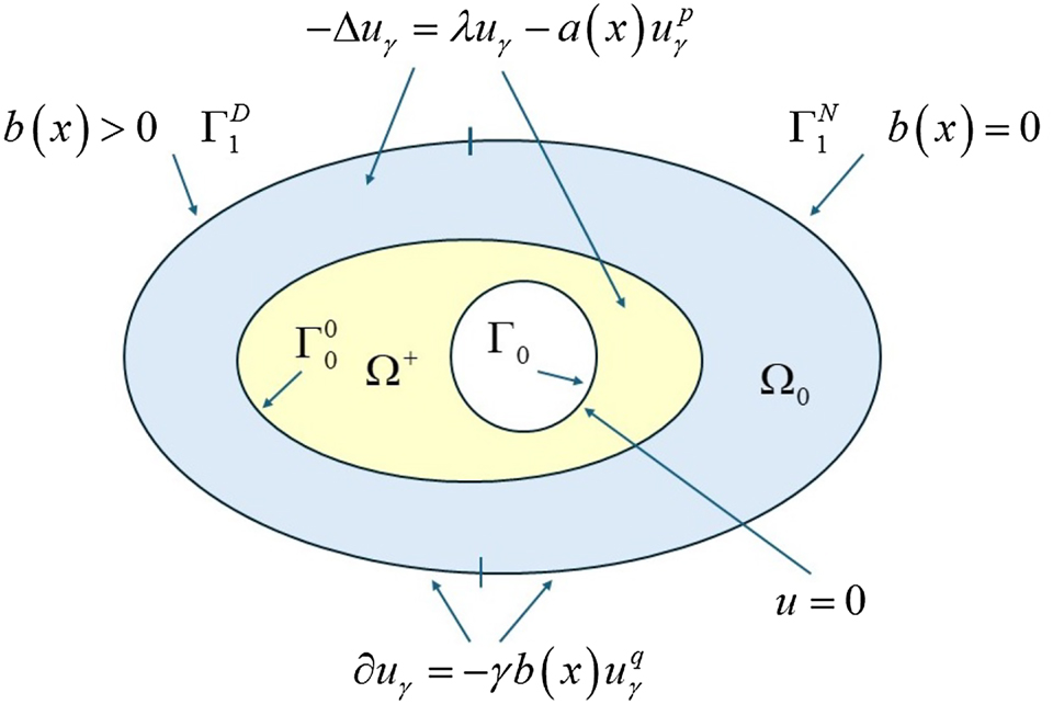
Configuration of Ω and
The existence and asymptotic behavior of positive solutions to elliptic boundary value problems with a bifurcation-continuation parameter in the boundary conditions has been extensively studied in previous works, such as [1], [2], [3], [4]. In this paper, we analyze the limiting profile of positive solutions to (1.1) as γ tends to infinity. Equation (1.1) models a logistic elliptic boundary value problem with nonlinear mixed boundary conditions, arising in the context of coastal fishery harvesting under spatially heterogeneous conditions (cf. [5]). Additionally, taking into account that the nonnegative solutions of (1.1) correspond to the steady states of positive solutions in the associated parabolic problem, (1.1) plays a key role in population dynamics with spatial heterogeneities. This is particularly relevant in scenarios where, due to the heterogeneous distribution of natural resources, some regions of the habitat boundary exhibit zero population flux, while others experience a nonlinear population flux.
To analyze the limiting behavior of the positive solutions to (1.1) as γ tends to infinity, we focus on the positive weak solutions of the following heterogeneous logistic elliptic boundary value problem, which involves mixed and glued Dirichlet-Neumann boundary conditions:
These weak solutions will play a crucial role in our analysis.
The main result of this work (Theorem 1.1) states that if the parameter λ belongs to a suitable interval, to specify later, the limiting behavior of the positive solutions to (1.1) in H 1(Ω) as γ tends to infinity coincides with the unique positive weak solution of (1.5).
Before stating our main findings, we introduce some notations and previous results. Let us denote
and let
By construction if
By a positive weak solution of (1.5) we mean any function
and such that for each
In particular, taking
Hereafter we denote
and by
In the sequel we will say that a function
Let us consider the eigenvalue problem
By a principal eigenvalue of (1.6) we mean any eigenvalue of it which possesses a one-signed eigenfunction and in particular a positive eigenfunction. Owing to the results in [6], Theorem 12.1] it is known that (1.6) possesses a unique principal eigenvalue, denoted in the sequel by
and in addition
Also, hereafter we denote
A function
with some of the inequalities strict.
Now, let us consider the eigenvalue problem with mixed and glued Dirichlet-Neumann boundary conditions on Γ1 given by
A function φ is said to be a weak solution of (1.7) if
The value μ is an eigenvalue of (1.7), if there exists a weak solution φ ≠ 0 of (1.7) associated to μ. In that case, it is said that φ is a weak eigenfunction of (1.7) associated to the eigenvalue μ. By a principal eigenvalue of (1.7) we mean any eigenvalue of it which possesses a one-signed eigenfunction and in particular a positive eigenfunction.
Owing to the results in [7], Theorem 1.1] it is known that (1.7) possesses a unique principal eigenvalue, denoted in the sequel by
Moreover,
(cf. [7], (2.27)]). In the same way, substituting in (1.7) Ω by Ω0 and
where
Moreover, owing to [7], Corollary 3.5] and [8], Proposition 3.2] it is known that
and
but no clear monotonicity relationship exists between
The problem of ascertaining the limiting profile of the positive solutions of (1.1) when γ tends to infinity was already analyzed in [3], in the particular case when the potential b is a positive potential bounded away from zero on Γ1, that is,
Owing to the fact that under assumptions of [3], Th.1.1 and Th.1.2] for each fixed
The following is the main result of this work
Theorem 1.1.
Under the general assumptions (1.2), (1.3) and (1.4), assume in addition that
and
Then,
where u γ and u* stand for the unique positive solution of (1.1) and (1.5), respectively.
Figure 2 shows the behavior of the limiting profile u* of the positive solution u γ of (1.1) when γ tends to infinity versus the profile of the potential b(x) on Γ1.
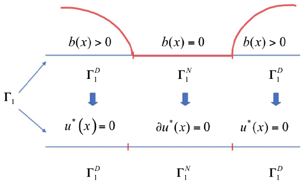
Behavior of u* on Γ1 versus profile of b(x)
Now, Theorem 1.1 asserts that if (1.2), (1.3) and (1.4) hold, then, the contrary to the cases analyzed in [3], the bifurcation of (1.1) to positive solutions from the trivial branch (γ, u) = (γ, 0) when γ tends to infinity fails, since (1.15) holds.
Remark 1.1.
Owing to (1.10) and (1.11) we have that
Moreover, it is known that when
In the particular case when the potential
Theorem 1.2.
Under the general conditions (1.2) and (1.3), assume in addition that
Then,
where u
γ
stands for the unique positive solution of (1.1) and
Then, the results obtained in [3], Th.1.1, Th.1.2] together with Theorem 1.1 and Theorem 1.2 show that the profile of the positive potential b on the boundary condition plays a crucial role in the shape of the limiting profile u* of the positive solutions of (1.1) when γ tends to infinity.
The main technical tools used to carry out the mathematical analysis of this work are functional and monotonicity techniques.
The structure of this paper is as follows. Section 2 collects some previous results that are going to be used throughout this work, and Section 3 contains the proofs of Theorem 1.1 and Theorem 1.2.
2 Preliminaries, notations and previous results
Let us denote by Λ
γ
, Λ* and
and for each
Let
and
Owing to (2.2) and (2.3) next result follows from [10], Theorem 1.1-i)].
Proposition 2.1.
For each γ > 0, (1.1) possesses a positive solution if, and only if
that is
Moreover, for each λ ∈ Λ γ , the positive solution of (1.1) is unique and strongly positive in Ω. In the sequel we will denote it by u γ . Furthermore,
Next result provides us with a comparison method and it is proved following similar arguments to those used in the proof of [11], Proposition 3.2].
Proposition 2.2.
Assume (2.4) and let
As for the existence and uniqueness of positive solution of (1.5), next result follows adapting to our framework the arguments given in [12], Theorem 3].
Proposition 2.3.
Problem (1.5) admits a positive weak solution
that is,
In this case, the solution u* is unique.
3 Proofs of Theorem 1.1 and Theorem 1.2
Proof of Theorem 1.1:
Pick λ satisfying (1.14). Since any positive constant is a positive strict supersolution of the problem
To prove the result we will show that (1.15) holds for every sequence of real numbers
Subsequently, we fix a sequence satisfying (3.1) and set
Since (3.1) holds, we can assume without loss of generality that
Also, due to (1.10), (1.11), (1.13), (1.14), (2.5) and (2.6), we have that
Then, it follows from Proposition 2.1 and (2.1), the existence for each n ≥ 1 of a unique positive solution of (1.1) and (1.18), u
n
and
In particular,
Also, owing to (3.3), it follows from Proposition 2.3 the existence of a unique positive weak solution
Moreover, thanks to (3.4) it is clear that the function
Also, thanks to (3.2), it is easy to prove that u 1 is a positive strict supersolution of (1.1) for each n ≥ 2 and hence, it follows from Proposition 2.2 that
Thus, (3.5) and (3.6) imply that
On the other hand, multiplying (1.1) by u n and integrating by parts it becomes apparent that
and hence, since u n is strongly positive in Ω, a⪈0, b⪈0 and γ n > 0, it follows from (3.7) and (3.8) that
Now, owing to the fact that u 1 ∈ W 2(Ω) ⊂ L ∞ (Ω), it follows from (3.7) and (3.9) the existence of a constant M > 0 such that
Moreover, owing to (3.7) and (3.10), it is apparent that along some subsequence, again labeled by n,
In the sequel we will restrict ourselves to dealing with functions of this subsequence.
Owing to (3.7) and (3.8) we have that
Thus, since u 1 ∈ L ∞ (Ω), it follows from (3.12) that there exists a constant C > 0 such that
and hence, (3.13) and (3.1) imply that along some subsequence, again labeled by n,
In particular, since b(x) > 0 for all
On the other hand, since the injection operator H 1(Ω)↪L 2(Ω) is compact, it follows from (3.10) the existence of u ∈ L 2(Ω) and a subsequence of u n , n ≥ 1, again labeled by n, such that
To complete the rest of the proof it suffices to prove that (3.11) and (3.15) imply that u = u* and
since this argument can be repeated along any subsequence of the original sequence. To prove it, set
By construction,
and owing to (3.7) the following holds
Also, owing to (3.16), it follows from the continuity of the trace operator on Γ1,
Now, since by construction v n provides us with a positive solution of the problem
(3.7), (3.16) and (3.19) imply that
for
Then, owing to (3.18) and (3.20), it follows from the L p -elliptic estimates of Agmon, Douglis and Nirenberg [14] the existence of a constant C 3 > 0 such that
Moreover, taking into account the continuity of the trace operator on Γ1,
Since H 1(Ω) is compactly embedded in L 2(Ω), it follows from (3.16) the existence of v ∈ L 2(Ω) and a subsequence of v n , again labeled by n, such that
In particular,
and since v n > 0, n ≥ 1, we obtain that
In addition, due to the compactness of the injection operator from
Now, let K be any compact subset of
Then, owing to (3.19) the following holds on K
Also, since (3.11) holds, there exists
Now, (3.25) and (3.26) imply that
and hence,
Then, (3.27) and (3.22) imply that for n ≥ n 0 the following holds
Now, owing to (3.1), letting n → ∞ in (3.28) gives
and since L 2q (K) ⊂ L 2(K) we have that
Thus, (3.11) and (3.29) imply that
in any compact subset
Now we are going to prove that since (3.30) holds in any compact subset
In particular
Indeed, given any ɛ > 0, take a compact subet K contained in
where |⋅| stands for the Lebesgue measure in L
2(Γ1) and
Now, owing to (3.17), (3.32) and (3.33), it is apparent that
Thus, for any ɛ > 0 there exists
Then, since by construction
We now show that v n is a Cauchy sequence in H 1(Ω). Indeed, since (3.19) holds, it is apparent that
Then, multiplying the partial differential equation of (3.34) by v m − v k and integrating by parts gives
Now, thanks to (3.6), (3.16), (3.22) and applying the Holder’s inequality, the following estimates hold:
Finally, substituting (3.36), (3.37) and (3.38) in (3.35), it follows from (3.23) and (3.24) that for any ɛ > 0 there exists
which proves that v n , n ≥ 1 is a Cauchy sequence in H 1(Ω). Now, combining this fact with (3.16) and (3.23) give
and in particular, it shows that v ∈ H 1(Ω).
We now ascertain the behavior of v on ∂Ω. We already know that v
n
− v ∈ H
1(Ω). Let
and owing to (3.39) it is apparent that
Now, since
and therefore, since v ∈ H 1(Ω), we obtain that
Moreover, since v n ⪈0, n ≥ 1, it follows from (3.39) that
that is, v(x) ≥ 0 almost everywhere in Ω, but v ≠ 0. On the other hand, the following holds for each n ≥ 1
where L > 0 is the limit defined by (3.11). Then, it follows from (3.11) and (3.15) that
and therefore, (3.23) and (3.41) imply that
In particular, (3.40) and (3.42) imply that
Now we show that u provides us with a weak solution of (1.5). We already now that
It should be noted that since
it is apparent that
Then, taking into account (3.7), (3.11), (3.15) and (3.39), and letting n → ∞ in (3.44) gives
Now, multiplying (3.45) by L and taking into account (3.42), it is apparent that for each
In particular, taking
and therefore, (3.43), (3.46) and (3.47) conclude that
and owing to (3.39) the following holds
Now, (3.10) and (3.48) imply that
and letting n → ∞ in (3.49), it follows from (3.11) and (3.39) that (1.15) holds along some subsequence. Therefore, since the same argument works along any subsequence, the proof is completed.
□
Proof of Theorem 1.2:
Assume that
In this case we have that
and for each fixed λ ∈ Λ γ , (1.1) possesses a unique positive solution, which we denote by u γ . Owing to (1.10), (2.1) and (3.51) we have that for each γ > 0 the following holds
Pick λ satisfying (1.16). In the same way as in the proof of Theorem 1.1, to prove (1.17) we will show that (1.17) holds for any sequence of real numbers
Indeed, since
(cf. (3.19)), taking into account (3.50) and the fact that
Then, owing to (3.22) it follows from (3.53) that
for some constant C 4 > 0. Now, owing to the fact that lim n→∞ γ n = ∞, letting n → ∞ in (3.54) gives
and since L 2q (Γ1) ⊂ L 2(Γ1), it is apparent that
Now, taking into account (3.11), it follows from (3.55) that (3.52) holds. This completes the proof.
□
-
Research ethics: Not applicable.
-
Informed consent: Not applicable.
-
Author contributions: The author confirms the sole responsibility for the conception of the study, presented results and manuscript preparation.
-
Use of Large Language Models, AI and Machine Learning Tools: None declared.
-
Conflict of interest: Author states no conflict of interest.
-
Research funding: The author has been supported by the Research Grant PID2021-123343NB-I00 of the Ministry of Science and Innovation of Spain.
-
Data availability: Not applicable.
References
[1] J. Garcia-Melián, J. C. Sabina de Lis, and J. D. Rossi, A bifurcation problem governed by the boundary condition I, NoDEA Nonlinear Differential Equations Appl. 14 (2007), 499–525, https://doi.org/10.1007/s00030-007-4064-x.Search in Google Scholar
[2] J. Garcia-Melián, J. D. Rossi, and J. C. Sabina de Lis, A bifurcation problem governed by the boundary condition II, Proc. London Math. Soc. 94 (2007), no. 1, 1–25, https://doi.org/10.1112/plms/pdl001.Search in Google Scholar
[3] S. Cano-Casanova, Heterogeneous elliptic BVPs with a bifurcation-continuation parameter in the nonlinear mixed boundary conditions, Adv. Nonlinear Stud. 20 (2020), no. 1, 31–51, https://doi.org/10.1515/ans-2019-2051.Search in Google Scholar
[4] K. Umezu, Logisitc elliptic equations with a nonlinear boundary condition arising from coastal fishery harvesting, Nonlinear Anal. Real World Appl. 70 (2023), 103788, DOI https://doi.org/10.1016/j.nonrwa.2022.103788.Search in Google Scholar
[5] D. Grass, H. Uecker, and T. Upmann, Optimal fishery with coastal catch, Nat. Resour. Model 32 (2019), no. 4, e12235, https://doi.org/10.1111/nrm.12235.Search in Google Scholar
[6] H. Amann, Dual semigroups and second order linear elliptic boundary value problems, Israel J. Math. 45 (1983), 225–254, https://doi.org/10.1007/bf02774019.Search in Google Scholar
[7] S. Cano-Casanova, Principal eigenvalues of elliptic BVPs with glued Dirichlet-Robin mixed boundary conditions. Large potentials on the boundary conditions, J. Math. Anal. Appl. 491 (2020), no. 2, 124364, DOI https://doi.org/10.1016/j.jmaa.2020.124364.Search in Google Scholar
[8] S. Cano-Casanova and J. López-Gómez, Properties of the principal eigenvalues of a general class on non-classical mixed boundary value problems, J. Differential Equations 178 (2002), 123–211.10.1006/jdeq.2000.4003Search in Google Scholar
[9] J. M. Fraile, P. Koch Medina, J. López-Gómez, and S. Merino, Elliptic eigenvalue problems and unbounded continua of positive solutions of a semilinear elliptic equation, J. Differential Equations 127 (1996), no. 1, 295–319.10.1006/jdeq.1996.0071Search in Google Scholar
[10] S. Cano-Casanova, Influence of the spatial heterogeneities in the existence of positive solutions of logistic BVPs with sublinear mixed boundary conditions, Rend. Istit. Mat. Univ. Trieste 52 (2020), 163–191.Search in Google Scholar
[11] S. Cano-Casanova, Nonlinear mixed boundary conditions in BVPs of Logistic type with spatial heterogeneities and a nonlinear flux on the boundary with arbitrary sign. The case p > 2q − 1, J. Differential Equations 256 (2014), 82–107, https://doi.org/10.1016/j.jde.2013.08.011.Search in Google Scholar
[12] J. Garcia-Melián, J. D. Rossi, and J. C. Sabina de Lis, Existence and uniqueness of positive solutions to elliptic problems with sublinear mixed boundary conditions, Commun. Contemp. Math. 11 (2009), no. 4, 585–613, https://doi.org/10.1142/s0219199709003508.Search in Google Scholar
[13] J. López-Gómez, The maximum principle and the existence of principal eigenvalues for some linear weighted boundary value problems, J. Differential Equations 127 (1996), no. 1, 263–294, https://doi.org/10.1006/jdeq.1996.0070.Search in Google Scholar
[14] S. Agmon, A. Douglis, and L. Nirenberg, Estimates near the boundary for solutions of elliptic partial differential equations satisfying general boundary conditions, Comm. Pure Appl. Math. 12 (1959), 623–727, https://doi.org/10.1002/cpa.3160120405.Search in Google Scholar
© 2025 the author(s), published by De Gruyter, Berlin/Boston
This work is licensed under the Creative Commons Attribution 4.0 International License.
Articles in the same Issue
- On I-convergence of nets of functions in fuzzy metric spaces
- Special Issue on Contemporary Developments in Graphs Defined on Algebraic Structures
- Forbidden subgraphs of TI-power graphs of finite groups
- Finite group with some c#-normal and S-quasinormally embedded subgroups
- Classifying cubic symmetric graphs of order 88p and 88p 2
- Two-sided zero-divisor graphs of orientation-preserving and order-decreasing transformation semigroups
- Simplicial complexes defined on groups
- Further results on permanents of Laplacian matrices of trees
- Algebra
- Classes of modules closed under projective covers
- On the dimension of the algebraic sum of subspaces
- Green's graphs of a semigroup
- On an uncertainty principle for small index subgroups of finite fields
- On a generalization of I-regularity
- Algorithm and linear convergence of the H-spectral radius of weakly irreducible quasi-positive tensors
- The hyperbolic CS decomposition of tensors based on the C-product
- On weakly classical 1-absorbing prime submodules
- Equational characterizations for some subclasses of domains
- Algebraic Geometry
- Spin(8, ℂ)-Higgs bundles fixed points through spectral data
- Embedding of lattices and K3-covers of an Enriques surface
- Kodaira-Spencer maps for elliptic orbispheres as isomorphisms of Frobenius algebras
- Applications in Computer and Information Sciences
- Dynamics of particulate emissions in the presence of autonomous vehicles
- Exploring homotopy with hyperspherical tracking to find complex roots with application to electrical circuits
- Category Theory
- The higher mapping cone axiom
- Combinatorics and Graph Theory
- 𝕮-inverse of graphs and mixed graphs
- On the spectral radius and energy of the degree distance matrix of a connected graph
- Some new bounds on resolvent energy of a graph
- Coloring the vertices of a graph with mutual-visibility property
- Ring graph induced by a ring endomorphism
- A note on the edge general position number of cactus graphs
- Complex Analysis
- Some results on value distribution concerning Hayman's alternative
- Freely quasiconformal and locally weakly quasisymmetric mappings in metric spaces
- A new result for entire functions and their shifts with two shared values
- On a subclass of multivalent functions defined by generalized multiplier transformation
- Singular direction of meromorphic functions with finite logarithmic order
- Growth theorems and coefficient bounds for g-starlike mappings of complex order λ
- Refinements of inequalities on extremal problems of polynomials
- Control Theory and Optimization
- Averaging method in optimal control problems for integro-differential equations
- On superstability of derivations in Banach algebras
- The robust isolated calmness of spectral norm regularized convex matrix optimization problems
- Observability on the classes of non-nilpotent solvable three-dimensional Lie groups
- Differential Equations
- The ill-posedness of the (non-)periodic traveling wave solution for the deformed continuous Heisenberg spin equation
- A note on the global existence and boundedness of an N-dimensional parabolic-elliptic predator-prey system with indirect pursuit-evasion interaction
- Blow-up of solutions for Euler-Bernoulli equation with nonlinear time delay
- Periodic or homoclinic orbit bifurcated from a heteroclinic loop for high-dimensional systems
- Regularity of weak solutions to the 3D stationary tropical climate model
- Local minimizers for the NLS equation with localized nonlinearity on noncompact metric graphs
- Global existence and blow-up of solutions to pseudo-parabolic equation for Baouendi-Grushin operator
- Bubbles clustered inside for almost-critical problems
- Existence and multiplicity of positive solutions for multiparameter periodic systems
- Existence of positive periodic solutions for evolution equations with delay in ordered Banach spaces
- On a nonlinear boundary value problems with impulse action
- Normalized ground-states for the Sobolev critical Kirchhoff equation with at least mass critical growth
- Multiple positive solutions to a p-Kirchhoff equation with logarithmic terms and concave terms
- Infinitely many solutions for a class of Kirchhoff-type equations
- Real and non-real eigenvalues of regular indefinite Sturm–Liouville problems
- Existence of global solutions to a semilinear thermoelastic system in three dimensions
- Limiting profile of positive solutions to heterogeneous elliptic BVPs with nonlinear flux decaying to negative infinity on a portion of the boundary
- Morse index of circular solutions for repulsive central force problems on surfaces
- Differential Geometry
- On tangent bundles of Walker four-manifolds
- Pedal and negative pedal surfaces of framed curves in the Euclidean 3-space
- Discrete Mathematics
- Eventually monotonic solutions of the generalized Fibonacci equations
- Dynamical Systems Ergodic Theory
- Dynamical properties of two-diffusion SIR epidemic model with Markovian switching
- A note on weighted measure-theoretic pressure
- Pullback attractors for a class of second-order delay evolution equations with dispersive and dissipative terms on unbounded domain
- Pullback attractor of the 2D non-autonomous magneto-micropolar fluid equations
- Functional Analysis
- Spectrum boundary domination of semiregularities in Banach algebras
- Approximate multi-Cauchy mappings on certain groupoids
- Investigating the modified UO-iteration process in Banach spaces by a digraph
- Tilings, sub-tilings, and spectral sets on p-adic space
- Continuity and essential norm of operators defined by infinite tridiagonal matrices in weighted Orlicz and l∞ spaces
-
A family of commuting contraction semigroups on
- q-Stirling sequence spaces associated with q-Bell numbers
- Chlodowsky variant of Bernstein-type operators on the domain
- Hyponormality on a weighted Bergman space of an annulus with a general harmonic symbol
- Characterization of derivations on strongly double triangle subspace lattice algebras by local actions
- Fixed point approaches to the stability of Jensen’s functional equation
- Geometry
- The regularity of solutions to the Lp Gauss image problem
- Solving the quartic by conics
- Group Theory
- On a question of permutation groups acting on the power set
- A characterization of the translational hull of a weakly type B semigroup with E-properties
- Harmonic Analysis
- Eigenfunctions on an infinite Schrödinger network
- Maximal function and generalized fractional integral operators on the weighted Orlicz-Lorentz-Morrey spaces
- Subharmonic functions and associated measures in ℝn
- Mathematical Logic, Model Theory and Foundation
- A topology related to implication and upsets on a bounded BCK-algebra
- Boundedness of fractional sublinear operators on weighted grand Herz-Morrey spaces with variable exponents
- Number Theory
- Fibonacci vector and matrix p-norms
- Recurrence for probabilistic extension of Dowling polynomials
- Carmichael numbers composed of Piatetski-Shapiro primes in Beatty sequences
- The number of rational points of some classes of algebraic varieties over finite fields
- Classification and irreducibility of a class of integer polynomials
- Decompositions of the extended Selberg class functions
- Joint approximation of analytic functions by the shifts of Hurwitz zeta-functions in short intervals
- Fibonacci Cartan and Lucas Cartan numbers
- Recurrence relations satisfied by some arithmetic groups
- The hybrid power mean involving the Kloosterman sums and Dedekind sums
- Numerical Methods
- A modified predictor–corrector scheme with graded mesh for numerical solutions of nonlinear Ψ-caputo fractional-order systems
- A kind of univariate improved Shepard-Euler operators
- Probability and Statistics
- Statistical inference and data analysis of the record-based transmuted Burr X model
- Multiple G-Stratonovich integral in G-expectation space
- p-variation and Chung's LIL of sub-bifractional Brownian motion and applications
- Real Analysis
- Chebyshev polynomials of the first kind and the univariate Lommel function: Integral representations
- Multiple solutions for a class of fourth-order elliptic equations with critical growth
- Majorization-type inequalities for (m, M, ψ)-convex functions with applications
- The evaluation of a definite integral by the method of brackets illustrating its flexibility
- Some new Fejér type inequalities for (h, g; α - m)-convex functions
- Some new Hermite-Hadamard type inequalities for product of strongly h-convex functions on ellipsoids and balls
- Topology
- Unraveling chaos: A topological analysis of simplicial homology groups and their foldings
- A generalized fixed-point theorem for set-valued mappings in b-metric spaces
- On SI2-convergence in T0-spaces
- Generalized quandle polynomials and their applications to stuquandles, stuck links, and RNA folding