Pedal and negative pedal surfaces of framed curves in the Euclidean 3-space
-
Kaixin Yao


Abstract
We define pedal and negative pedal surfaces of framed curves in the Euclidean 3-space and find that the loci of singularities of them are pedal and negative pedal curves, respectively. Moreover, we give sufficient conditions that pedal and negative pedal surfaces to be framed base surfaces. We also give a sufficient condition that negative pedal curves to be framed base curves.
1 Introduction
Curves or surfaces generated by curves are important branches in differential geometry. Some properties of the original curve can be reflected by the new curve or surface. For example, given a smooth regular curve with a vertex in the Euclidean plane, its evolute is singular at the point corresponding to the vertex of the original curve. There are also relations between curves and surfaces generated by the same curve. For a spatial curve, the singularity locus of its focal surface coincides with its evolute [1] (Figure 1).
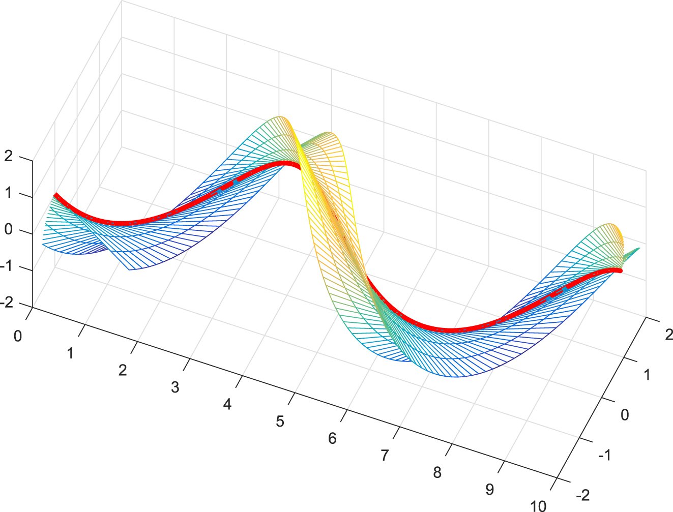
A focal surface (mesh) and an evolute (red).
People first considered that original curves are regular. In fact, there is a limitation. With the development of Legendre curves, people can deal with this kind of curves, which may have singularities, similarly to regular curves [2]. A Legendre curve can be determined by its invariants uniquely up to rigid motions. For a Legendre curve (Legendre immersion), its base curve is called a frontal (front). Lifting the dimension of the space, Honda and Takahashi defined framed curves in the Euclidean n-space [3]. There is more than one way to frame a curve and different frames can be used to research its properties [4]. One can find an adapted frame to make some questions easier. Honda and Takahashi defined the Frenet type frame along a framed base curve in the Euclidean 3-space [1],5]. So far, framed curves with Frenet type frames can be regarded as the generalization of Frenet curves.
Roulettes and pedal curves play an important role in the study of road-wheel pairs. Pedal curves have connections with moving wheels [6]. In astronomy, Kepler discovered the trace of a moving planet is an ellipse. The ellipse is called Kepler’s ellipse. Hamilton claimed that the pedal curve of Kepler’s ellipse relative to the focus is a circle [7]. That is to say the ellipse is the negative pedal curve of the circle. Later, pedal curves in different spaces have been studied by many researchers. People were first concerned about pedal curves of regular curves. They found the pedal curve is singular if the original curve has inflections or the pedal point lies on the original curve. Later, Nishimura defined pedal curves in n-dimensional sphere and studied normal forms for singularities of them [8],9]. Using the theory of Legendre curves, people defined pedal curves of fronts and frontals in the Euclidean plane [10],11]. It contains the case of regular plane curves. However, pedal curves of frontals may be not frontals. Tuncer et al. gave a sufficient condition when the pedal curve of a front is a frontal. We studied the pedal curves of framed curves with Frenet type frames in the Euclidean 3-space [12]. Li and the second author of this paper researched pedal-contrapedal curve pairs of fronts in the unit sphere and discussed their relationships with the involute-evolute curve pairs [13]. As for other spaces, such as Minkowski space and its submanifolds, pedal curves were defined and studied [14], [15], [16]. If the orthogonal projection is changed to the slant projection, one can get pedaloids in plane. There are some results about pedaloids in the Euclidean plane and the Lorentz plane [17], [18], [19]. Pedal curves in a plane have applications in physics. One can use pedal curves to generate coordinates, called pedal coordinates, to deal with some mechanical problems [20], [21], [22].
Naturally, there is an inverse problem: if we know a curve and a fixed point, how can we get a new curve such that its pedal curve relative to the fixed point is the given curve? The new curve is called the negative pedal curve or the primitive. Arnol’d researched the primitive of a hypersurface [23]. It is the envelope of the normal hyperplanes. Izumiya and Takeuchi introduced the primitivoids of plane curves, which are generalizations of primitives [24]. For n dimensional frontals in the (n + 1) dimensional Euclidean space, Janeczko and Nishimura defined their negative pedals [25]. This is the generalization of the case of Arnol’d.
In the Euclidean plane, the pedal curve is the envelope of a family of circles and the primitive is the envelope of a family of lines. Taking the pedal curve and taking the primitive can be regarded as inverse processes. We consider envelopes of a family of spheres and a family of planes in the Euclidean 3-space, call them the pedal surface and the negative pedal surface, respectively. Previously, people usually studied pedal surfaces of surfaces [26]. It is a transformation of the same dimension. We change the correspondence of dimension. Based on our previous work [12], we research pedal surfaces and negative pedal surfaces.
In the present paper, we define pedal surfaces, negative pedal surfaces and negative pedal curves of framed curves. The singular locus of the pedal surface is the pedal curve and the pedal point. For the singular locus of the negative pedal surface, if we can establish the Frenet type frame along it and take its pedal curve, then it is the original curve. So we call it the negative pedal curve. We get sufficient conditions when the pedal surface and the negative pedal surface are framed base surfaces. Finally, we give two examples to show connections among pedal curves, negative pedal curves, pedal surfaces and negative pedal surfaces.
All maps and manifolds considered here are differentiable of class C ∞ .
2 Preliminaries
Let
Definition 2.1
([3]). I is an interval of
For a framed curve (γ, ν 1, ν 2), define μ (t) = ν 1(t) × ν 2(t). Then { ν 1(t), ν 2(t), μ (t)} is a moving frame along γ(t). The Frenet type formulas are
where
The map
By the above definition, we know the linear combination of ν 1(t) and ν 2(t) is orthogonal to γ′(t). If (m(t), n(t)) ≠ (0, 0) for all t ∈ I, we take
Then (γ, n 1, n 2) is also a framed curve and n 1(t) × n 2(t) = μ (t). { n 1(t), n 2(t), μ (t)} is called the Frenet type frame along γ(t). The Frenet type formulas are
where
The map
In our previous paper, we have defined pedal curves of framed curves by orthogonal projection.
Definition 2.2
([12]). Let
We call p the pedal point.
Definition 2.3
([27]). U is an open domain in
Let
3 Pedal and negative pedal surfaces
Definition 3.1.
Let
The pedal surface
Suppose the point p satisfies (γ(t) − p ) ⋅ n 2(t) ≠ 0 for all t ∈ I. The negative pedal surface
Remark 3.2.
If the point
p
is on the tangent developable of γ, then the pedal surface
When the curve γ is regular, the two surfaces defined in Definition 3.1 can be both regarded as envelopes of families of surfaces.
Proposition 3.3.
Let
The pedal surface
If the point p satisfies (γ(t) − p ) ⋅ n 2(t) ≠ 0 for all t ∈ I, then the negative pedal surface
Proof.
(a) Define
Let
Define
Let
□
Definition 3.4.
Let
Now we consider singularities of the pedal surface and negative pedal surface.
Theorem 3.5.
Let
Suppose that the point p is not on the tangent developable of γ.
Suppose that the point p satisfies (γ(t) − p ) ⋅ n 2(t) ≠ 0 for all t ∈ I.
Proof.
(a) By calculation, we have
and
So (t
0, θ
0) is a singularity of
This means that
or
By calculation, we have
and
So (t
0, λ
0) is a singularity of
□
The pedal surface and negative pedal surface may have singular points. We give conditions when they are framed base surfaces. For framed base surfaces, please see [27].
Proposition 3.6.
Let
If p is not on the tangent developable of γ, then the pedal surface
Suppose that the point p satisfies (γ(t) − p ) ⋅ n 2(t) ≠ 0 for all t ∈ I. Then the negative pedal surface
Proof.
(a) Take
and
By Equations (1) and (2), we can check that
So
Take
and
By Equations (3) and (4), we can check that
So
Following propositions claim a fact that the negative pedal curve is also a framed base curve and the relation between the negative pedal curve and the pedal curve.
Proposition 3.7.
Let
Then
Proof.
We have
It is obvious that
Note that
and
We complete the proof. □
Proposition 3.8.
Let
Proof.
By Proposition 3.7, we know the binormal direction of
where sign is the signature function. Note that
So the pedal curve of
□
4 Examples
Here, we give two examples to show pedal and negative pedal surfaces of framed curves.
Example 4.1.
Let
with the curvature
Let p = 0. The pedal curve, negative pedal curve, pedal surface and negative pedal surface of (γ, n 1, n 2) relative to p are
and
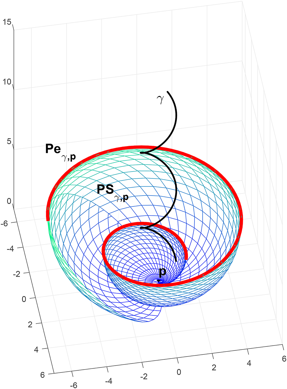
γ (black), its pedal curve (red) and pedal surface (mesh).
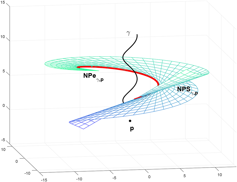
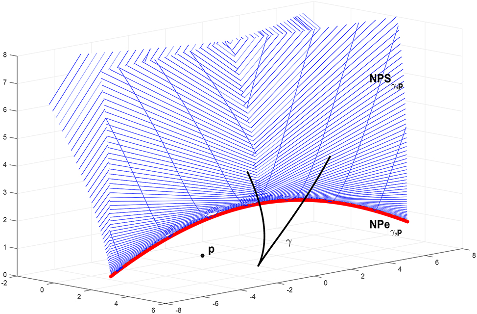
γ (black), its negative pedal curve (red) and negative pedal surface (mesh).
Example 4.2.
Let
with the curvature
Let p = 0. The pedal curve, negative pedal curve, pedal surface and negative pedal surface of (γ, n 1, n 2) relative to p are
and
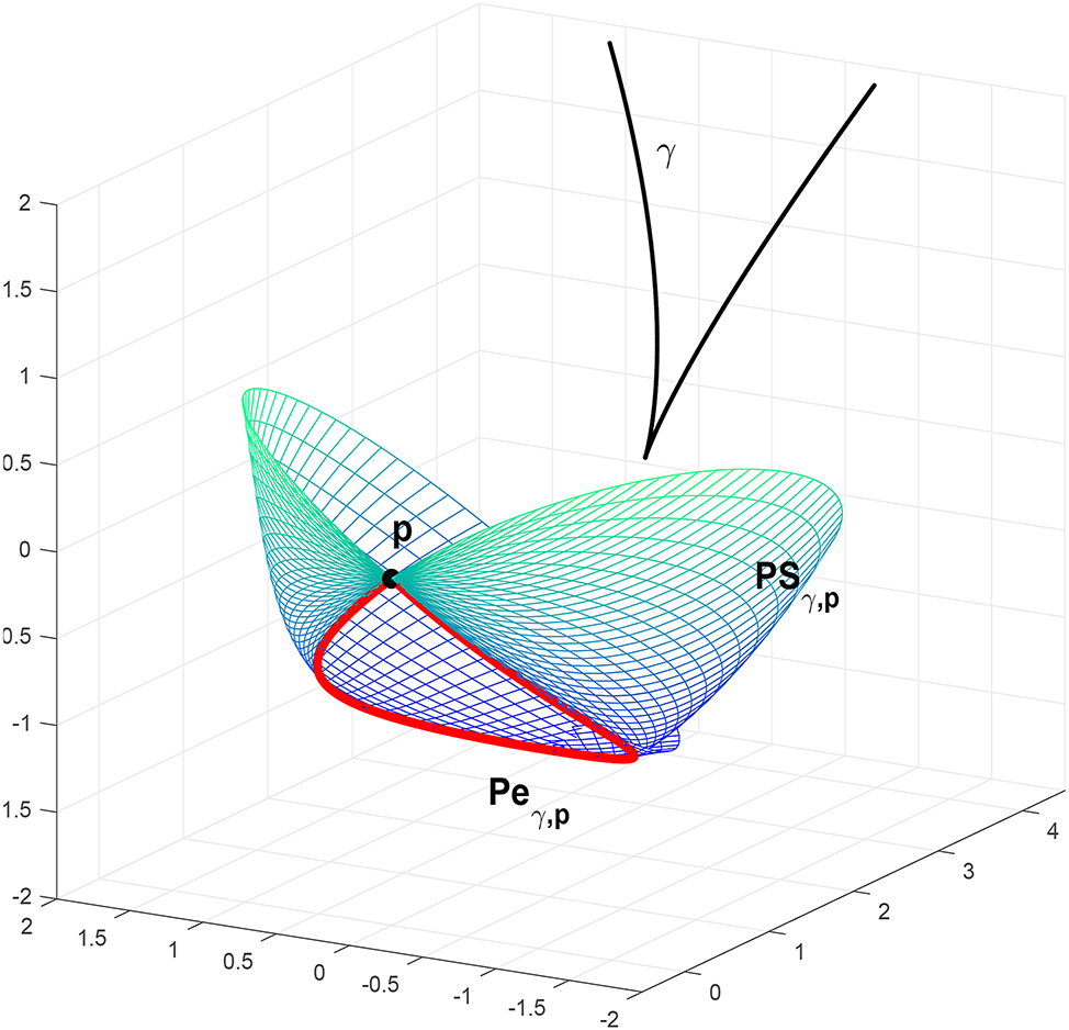
γ (black), its pedal curve (red) and pedal surface (mesh).
γ (black), its negative pedal curve (red) and negative pedal surface (mesh).
From above examples, we can see the singular locus of the pedal surface and the negative pedal surface. This is consistent with Theorem 3.5.
5 Conclusions
We define pedal and negative pedal surfaces of framed curves in the Euclidean 3-space. Their singular loci are pedal and negative pedal curves, respectively. The two surfaces are envelopes of families of spheres and planes, respectively. Moreover, we also give sufficient conditions when they can be framed base surfaces. As for negative pedal curves, we give the sufficient condition when they can be framed base curves and discuss their connection with pedal curves. The theoretical value of our research is the correspondence between curves and surfaces, which is different from the correspondence between manifolds with the same dimension in most previous studies.
Acknowledgments
The authors would like to thank the reviewers for helpful comments to improve the original manuscript.
-
Research ethics: Not applicable.
-
Informed consent: Not applicable.
-
Author contributions: Authors have accepted responsibility for the entire content of this manuscript and consented to its submission to the journal, reviewed all the results and approved the final version of the manuscript. KY wrote the main manuscript text. KY and DP reviewed and edited. DP funded.
-
Use of Large Language Models, AI and Machine Learning Tools: None declared.
-
Conflict of interest: Authors declare that there is no conflict of interest.
-
Research funding: This work was supported by the National Natural Science Foundation of China (Grant No. 11671070).
-
Data availability: Not applicable.
References
[1] S. Honda and M. Takahashi, Evolutes and focal surfaces of framed immersions in the Euclidean space, Proc. Roy. Soc. Edinburgh Sect. A 150 (2020), no. 1, 497–516, https://doi.org/10.1017/prm.2018.84.Suche in Google Scholar
[2] T. Fukunaga and M. Takahashi, Existence and uniqueness for Legendre curves, J. Geom. 104 (2013), no. 2, 297–307, https://doi.org/10.1007/s00022-013-0162-6.Suche in Google Scholar
[3] S. Honda and M. Takahashi, Framed curves in the Euclidean space, Adv. Geom. 16 (2016), no. 3, 265–276, https://doi.org/10.1515/advgeom-2015-0035.Suche in Google Scholar
[4] R. L. Bishop, There is more than one way to frame a curve, Amer. Math. Monthly 82 (1975), 246–251, https://doi.org/10.2307/2319846.Suche in Google Scholar
[5] S. Honda and M. Takahashi, Bertrand and Mannheim curves of framed curves in the 3-dimensional Euclidean space, Turkish J. Math. 44 (2020), no. 3, 883–899, https://doi.org/10.3906/mat-1905-63.Suche in Google Scholar
[6] F. Kuczmarski, Roads and wheels, roulettes and pedals, Amer. Math. Monthly 118 (2011), no. 6, 479–496, https://doi.org/10.4169/amer.math.monthly.118.06.479.Suche in Google Scholar
[7] J. Stávek, Kepler’s ellipse observed from Newton’s evolute (1687), Horrebow’s circle (1717), Hamilton’s pedal curve (1847), and two contrapedal curves (28.10.2018), Appl. Phys. Res. 10 (2018), no. 6, 90–101, https://doi.org/10.5539/apr.v10n6p90.Suche in Google Scholar
[8] T. Nishimura, Normal forms for singularities of pedal curves produced by non-singular dual curve germs in Sn, Geom. Dedicata 133 (2008), 59–66, https://doi.org/10.1007/s10711-008-9233-5.Suche in Google Scholar
[9] T. Nishimura, Singularities of pedal curves produced by singular dual curve germs in Sn, Demonstr. Math. 43 (2010), no. 2, 447–459, https://doi.org/10.1515/dema-2010-0216.Suche in Google Scholar
[10] Y. Li and D. Pei, Pedal curves of frontals in the Euclidean plane, Math. Methods Appl. Sci. 41 (2018), no. 5, 1988–1997, https://doi.org/10.1002/mma.4724.Suche in Google Scholar
[11] O. O. Tuncer, H. Ceyhan, İ. Gök, and F. N. Ekmekci, Notes on pedal and contrapedal curves of fronts in the Euclidean plane, Math. Methods Appl. Sci. 41 (2018), no. 13, 5096–5111, https://doi.org/10.1002/mma.5056.Suche in Google Scholar
[12] K. Yao, M. Li, E. Li, and D. Pei, Pedal and contrapedal curves of framed immersions in the Euclidean 3-space, Mediterr. J. Math. 20 (2023), no. 4, 204, https://doi.org/10.1007/s00009-023-02408-z.Suche in Google Scholar
[13] E. Li and D. Pei, Involute-evolute and pedal-contrapedal curve pairs on S2, Math. Methods Appl. Sci. 45 (2022), no. 18, 11986–12000, https://doi.org/10.1002/mma.6994.Suche in Google Scholar
[14] G. Aydın Şekerci, On evolutoids and pedaloids in Minkowski 3-space, J. Geom. Phys. 168 (2021), 104313, https://doi.org/10.1016/j.geomphys.2021.104313.Suche in Google Scholar
[15] Y. Li and O. O. Tuncer, On (contra)pedals and (anti)orthotomics of frontals in de Sitter 2-space, Math. Methods Appl. Sci. 46 (2023), no. 9, 11157–11171, https://doi.org/10.1002/mma.9173.Suche in Google Scholar
[16] Y. Li, Y. Zhu, and Q. Sun, Singularities and dualities of pedal curves in pseudo-hyperbolic and de Sitter space, Int. J. Geom. Methods Mod. Phys. 18 (2021), no. 1, 2150008. https://doi.org/10.1142/S0219887821500080.Suche in Google Scholar
[17] G. Aydın Şekerci and S. Izumiya, Evolutoids and pedaloids of Minkowski plane curves, Bull. Malays. Math. Sci. Soc. 44 (2021), no. 5, 2813–2834, https://doi.org/10.1007/s40840-021-01091-1.Suche in Google Scholar
[18] S. Izumiya and N. Takeuchi, Evolutoids and pedaloids of plane curves, Note Mat. 39 (2019), no. 2, 13–23, https://doi.org/10.1285/i15900932v39n2p13.Suche in Google Scholar
[19] Z. Yang, Y. Li, M. Erdoğdu, and Y. Zhu, Evolving evolutoids and pedaloids from viewpoints of envelope and singularity theory in Minkowski plane, J. Geom. Phys. 176 (2022), 104513, https://doi.org/10.1016/j.geomphys.2022.104513.Suche in Google Scholar
[20] P. Blaschke, Pedal coordinates, dark Kepler, and other force problems, J. Math. Phys. 58 (2017), no. 6, 063505, https://doi.org/10.1063/1.4984905.Suche in Google Scholar
[21] P. Blaschke, Pedal coordinates, solar sail orbits, Dipole drive and other force problems, J. Math. Anal. Appl. 506 (2022), no. 1, 125537, https://doi.org/10.1016/j.jmaa.2021.125537.Suche in Google Scholar
[22] P. Blaschke, F. Blaschke, and M. Blaschke, Pedal coordinates and free double linkage, J. Geom. Phys. 171 (2022), 104397, https://doi.org/10.1016/j.geomphys.2021.104397.Suche in Google Scholar
[23] V. I. Arnol’d, Dynamical Systems. VIII, Springer-Verlag, Berlin, 1993.Suche in Google Scholar
[24] S. Izumiya and N. Takeuchi, Primitivoids and inversions of plane curves, Beitr. Algebra Geom. 61 (2020), no. 2, 317–334, https://doi.org/10.1007/s13366-019-00472-9.Suche in Google Scholar
[25] S. Janeczko and T. Nishimura, Anti-orthotomics of frontals and their applications, J. Math. Anal. Appl. 487 (2020), no. 2, 124019, https://doi.org/10.1016/j.jmaa.2020.124019.Suche in Google Scholar
[26] M. Abdelatif, H. Nour Alldeen, H. Saoud, and S. Suorya, Finite type of the pedal of revolution surfaces in E3, J. Korean Math. Soc. 53 (2016), no. 4, 909–928. https://doi.org/10.4134/JKMS.j150336.Suche in Google Scholar
[27] T. Fukunaga and M. Takahashi, Framed surfaces in the Euclidean space, Bull. Braz. Math. Soc. (N.S.) 50 (2019), no. 1, 37–65, https://doi.org/10.1007/s00574-018-0090-z.Suche in Google Scholar
[28] A. Gray, E. Abbena, and S. Salamon, Modern Differential Geometry of Curves and Surfaces with Mathematica, 3rd ed., Chapman & Hall/CRC, Boca Raton, FL, 2006.Suche in Google Scholar
© 2025 the author(s), published by De Gruyter, Berlin/Boston
This work is licensed under the Creative Commons Attribution 4.0 International License.
Artikel in diesem Heft
- On I-convergence of nets of functions in fuzzy metric spaces
- Special Issue on Contemporary Developments in Graphs Defined on Algebraic Structures
- Forbidden subgraphs of TI-power graphs of finite groups
- Finite group with some c#-normal and S-quasinormally embedded subgroups
- Classifying cubic symmetric graphs of order 88p and 88p 2
- Two-sided zero-divisor graphs of orientation-preserving and order-decreasing transformation semigroups
- Simplicial complexes defined on groups
- Further results on permanents of Laplacian matrices of trees
- Algebra
- Classes of modules closed under projective covers
- On the dimension of the algebraic sum of subspaces
- Green's graphs of a semigroup
- On an uncertainty principle for small index subgroups of finite fields
- On a generalization of I-regularity
- Algorithm and linear convergence of the H-spectral radius of weakly irreducible quasi-positive tensors
- The hyperbolic CS decomposition of tensors based on the C-product
- On weakly classical 1-absorbing prime submodules
- Equational characterizations for some subclasses of domains
- Algebraic Geometry
- Spin(8, ℂ)-Higgs bundles fixed points through spectral data
- Embedding of lattices and K3-covers of an Enriques surface
- Kodaira-Spencer maps for elliptic orbispheres as isomorphisms of Frobenius algebras
- Applications in Computer and Information Sciences
- Dynamics of particulate emissions in the presence of autonomous vehicles
- Exploring homotopy with hyperspherical tracking to find complex roots with application to electrical circuits
- Category Theory
- The higher mapping cone axiom
- Combinatorics and Graph Theory
- 𝕮-inverse of graphs and mixed graphs
- On the spectral radius and energy of the degree distance matrix of a connected graph
- Some new bounds on resolvent energy of a graph
- Coloring the vertices of a graph with mutual-visibility property
- Ring graph induced by a ring endomorphism
- A note on the edge general position number of cactus graphs
- Complex Analysis
- Some results on value distribution concerning Hayman's alternative
- Freely quasiconformal and locally weakly quasisymmetric mappings in metric spaces
- A new result for entire functions and their shifts with two shared values
- On a subclass of multivalent functions defined by generalized multiplier transformation
- Singular direction of meromorphic functions with finite logarithmic order
- Growth theorems and coefficient bounds for g-starlike mappings of complex order λ
- Refinements of inequalities on extremal problems of polynomials
- Control Theory and Optimization
- Averaging method in optimal control problems for integro-differential equations
- On superstability of derivations in Banach algebras
- The robust isolated calmness of spectral norm regularized convex matrix optimization problems
- Observability on the classes of non-nilpotent solvable three-dimensional Lie groups
- Differential Equations
- The ill-posedness of the (non-)periodic traveling wave solution for the deformed continuous Heisenberg spin equation
- A note on the global existence and boundedness of an N-dimensional parabolic-elliptic predator-prey system with indirect pursuit-evasion interaction
- Blow-up of solutions for Euler-Bernoulli equation with nonlinear time delay
- Periodic or homoclinic orbit bifurcated from a heteroclinic loop for high-dimensional systems
- Regularity of weak solutions to the 3D stationary tropical climate model
- Local minimizers for the NLS equation with localized nonlinearity on noncompact metric graphs
- Global existence and blow-up of solutions to pseudo-parabolic equation for Baouendi-Grushin operator
- Bubbles clustered inside for almost-critical problems
- Existence and multiplicity of positive solutions for multiparameter periodic systems
- Existence of positive periodic solutions for evolution equations with delay in ordered Banach spaces
- On a nonlinear boundary value problems with impulse action
- Normalized ground-states for the Sobolev critical Kirchhoff equation with at least mass critical growth
- Multiple positive solutions to a p-Kirchhoff equation with logarithmic terms and concave terms
- Infinitely many solutions for a class of Kirchhoff-type equations
- Real and non-real eigenvalues of regular indefinite Sturm–Liouville problems
- Existence of global solutions to a semilinear thermoelastic system in three dimensions
- Limiting profile of positive solutions to heterogeneous elliptic BVPs with nonlinear flux decaying to negative infinity on a portion of the boundary
- Morse index of circular solutions for repulsive central force problems on surfaces
- Differential Geometry
- On tangent bundles of Walker four-manifolds
- Pedal and negative pedal surfaces of framed curves in the Euclidean 3-space
- Discrete Mathematics
- Eventually monotonic solutions of the generalized Fibonacci equations
- Dynamical Systems Ergodic Theory
- Dynamical properties of two-diffusion SIR epidemic model with Markovian switching
- A note on weighted measure-theoretic pressure
- Pullback attractors for a class of second-order delay evolution equations with dispersive and dissipative terms on unbounded domain
- Pullback attractor of the 2D non-autonomous magneto-micropolar fluid equations
- Functional Analysis
- Spectrum boundary domination of semiregularities in Banach algebras
- Approximate multi-Cauchy mappings on certain groupoids
- Investigating the modified UO-iteration process in Banach spaces by a digraph
- Tilings, sub-tilings, and spectral sets on p-adic space
- Continuity and essential norm of operators defined by infinite tridiagonal matrices in weighted Orlicz and l∞ spaces
-
A family of commuting contraction semigroups on
- q-Stirling sequence spaces associated with q-Bell numbers
- Chlodowsky variant of Bernstein-type operators on the domain
- Hyponormality on a weighted Bergman space of an annulus with a general harmonic symbol
- Characterization of derivations on strongly double triangle subspace lattice algebras by local actions
- Fixed point approaches to the stability of Jensen’s functional equation
- Geometry
- The regularity of solutions to the Lp Gauss image problem
- Solving the quartic by conics
- Group Theory
- On a question of permutation groups acting on the power set
- A characterization of the translational hull of a weakly type B semigroup with E-properties
- Harmonic Analysis
- Eigenfunctions on an infinite Schrödinger network
- Maximal function and generalized fractional integral operators on the weighted Orlicz-Lorentz-Morrey spaces
- Subharmonic functions and associated measures in ℝn
- Mathematical Logic, Model Theory and Foundation
- A topology related to implication and upsets on a bounded BCK-algebra
- Boundedness of fractional sublinear operators on weighted grand Herz-Morrey spaces with variable exponents
- Number Theory
- Fibonacci vector and matrix p-norms
- Recurrence for probabilistic extension of Dowling polynomials
- Carmichael numbers composed of Piatetski-Shapiro primes in Beatty sequences
- The number of rational points of some classes of algebraic varieties over finite fields
- Classification and irreducibility of a class of integer polynomials
- Decompositions of the extended Selberg class functions
- Joint approximation of analytic functions by the shifts of Hurwitz zeta-functions in short intervals
- Fibonacci Cartan and Lucas Cartan numbers
- Recurrence relations satisfied by some arithmetic groups
- The hybrid power mean involving the Kloosterman sums and Dedekind sums
- Numerical Methods
- A modified predictor–corrector scheme with graded mesh for numerical solutions of nonlinear Ψ-caputo fractional-order systems
- A kind of univariate improved Shepard-Euler operators
- Probability and Statistics
- Statistical inference and data analysis of the record-based transmuted Burr X model
- Multiple G-Stratonovich integral in G-expectation space
- p-variation and Chung's LIL of sub-bifractional Brownian motion and applications
- Real Analysis
- Chebyshev polynomials of the first kind and the univariate Lommel function: Integral representations
- Multiple solutions for a class of fourth-order elliptic equations with critical growth
- Majorization-type inequalities for (m, M, ψ)-convex functions with applications
- The evaluation of a definite integral by the method of brackets illustrating its flexibility
- Some new Fejér type inequalities for (h, g; α - m)-convex functions
- Some new Hermite-Hadamard type inequalities for product of strongly h-convex functions on ellipsoids and balls
- Topology
- Unraveling chaos: A topological analysis of simplicial homology groups and their foldings
- A generalized fixed-point theorem for set-valued mappings in b-metric spaces
- On SI2-convergence in T0-spaces
- Generalized quandle polynomials and their applications to stuquandles, stuck links, and RNA folding