Hybrid white shark optimizer with differential evolution for training multi-layer perceptron neural network
-
Hussam N. Fakhouri
 ,
Abedelraouf Istiwi
,
Abedelraouf Istiwi

Abstract
This study presents a novel hybrid optimization algorithm combining the white shark optimizer (WSO) with differential evolution (DE), referred to as WSODE, for training multi-layer perceptron (MLP) neural networks and solving systems design problems. The structure of WSO, while effective in exploitation due to its wavy motion-based search, suffers from limited exploration capability. This limitation arises from WSO’s reliance on local search behaviors, where it tends to focus on a narrow region of the search space, reducing the diversity of solutions and increasing the likelihood of premature convergence. To address this, DE is integrated with WSO (WSODE) to enhance exploration by introducing mutation and crossover operations, which increase diversity and enable the algorithm to escape local optima. The performance of WSODE is evaluated on the CEC2022, CEC2021, and CEC2017 benchmark functions and compared against several state-of-the-art optimizers. The results demonstrate that WSODE consistently achieves superior or competitive performance, with faster convergence rates and higher solution quality across diverse benchmarks. Specifically, on the CEC2022 suite, WSODE ranked first or second across multiple functions, including high-dimensional, multi-modal, and deceptive landscapes and significantly outperforming other algorithms like WOA and SHO. On the CEC2021 suite, WSODE ranked first in several complex functions, such as C6 and C10, with mean values of
1 Introduction
Metaheuristics are advanced, high-level strategies designed to efficiently explore solution spaces in search of optimal or near-optimal solutions for complex optimization problems [1]. They are inherently problem-independent, which permits their application across a vast range of domains, from engineering design to machine learning and logistics [2]. Despite their robust capabilities, traditional metaheuristic algorithms face notable challenges that limit their effectiveness, particularly in high-dimensional, multi-modal landscapes. One such limitation is the tendency of many metaheuristics to converge prematurely, often becoming trapped in local optima, especially in cases where complex landscapes or multiple optima are present [3]. This weakness arises from the balance these algorithms attempt to strike between exploration (searching new areas of the solution space) and exploitation (refining existing solutions); traditional metaheuristics frequently struggle to maintain this balance, leading to suboptimal performance in scenarios with rugged search landscapes [4].
The high computational cost associated with some metaheuristics presents an additional challenge, particularly when dealing with large-scale, dynamic, or time-sensitive applications [5]. Many traditional algorithms suffer from a lack of efficiency when scaling to large problems, resulting in extended computation times and high resource consumption [6]. This inefficiency limits their practicality in real-world applications requiring quick decision-making or real-time adaptability. Furthermore, some metaheuristics lack the flexibility needed to address multiobjective optimization, where multiple conflicting objectives must be optimized simultaneously [7]. While multiobjective optimization is crucial in fields such as environmental management, financial portfolio optimization, and engineering design, traditional metaheuristics often fail to effectively balance these objectives and produce a comprehensive set of Pareto-optimal solutions [8].
These limitations underscore the need for advanced hybrid approaches that can enhance exploration–exploitation capabilities, reduce computational costs, and better address multiobjective optimization challenges [9]. Hybrid metaheuristics, which combine the strengths of multiple algorithms, have emerged as a promising solution to these challenges. By integrating complementary strategies, hybrid algorithms aim to leverage the exploration power of one approach with the exploitation efficiency of another, thus mitigating the weaknesses inherent in traditional algorithms [10]. This study contributes to this evolution by proposing a hybrid differential evolution-white shark optimizer (WSODE), a novel algorithm designed to address the weaknesses of traditional metaheuristics and extend their applicability across high-dimensional and multiobjective optimization problems.
In addition to traditional optimization applications, metaheuristics have found significant roles in complex, domain-specific tasks. In engineering, they are frequently employed for design optimization, system modeling, and process optimization, addressing challenges from structural design to energy management and manufacturing [11]. In computer science, metaheuristics support tasks such as feature selection, network design, and software testing, showcasing their versatility and domain adaptability [5]. The evolution of these algorithms, driven by continuous advancements in hybridization and adaptability, emphasizes their role in modern optimization landscapes, marking them as indispensable tools in solving increasingly complex real-world problems [12].
In the field of machine learning, optimization algorithms are fundamental to the training and tuning of models, particularly neural networks [13]. Machine learning has revolutionized numerous domains by enabling systems to learn patterns from data and make intelligent decisions. At the heart of many machine learning models are neural networks, which are inspired by the structure and function of the human brain. These networks, especially multi-layer perceptrons (MLPs), are widely used due to their ability to approximate complex functions and handle various types of data [14].
MLPs are a type of feed-forward neural network consisting of an input layer, one or more hidden layers, and an output layer [15]. Each neuron in a layer is connected to every neuron in the subsequent layer, with each connection having an associated weight. The training process of MLPs involves adjusting these weights to minimize the difference between the predicted output and the actual target values. This process requires efficient optimization techniques to navigate the high-dimensional and often nonconvex search space, making the choice of optimization algorithm critical for the network’s performance [16].
Despite their potential, training neural networks effectively remains a challenging task. The optimization landscape of neural networks is complex, characterized by numerous local minima and saddle points. Therefore, the optimizer’s ability to explore the search space thoroughly and exploit promising regions is crucial. DE is known for its robustness in global optimization, utilizing population-based search strategies and mutation operations to explore the search space. On the other hand, the WSO mimics the hunting behavior of white sharks, offering adaptive strategies for exploration and exploitation.
This research introduces a novel hybrid optimization algorithm, the WSODE, which strategically integrates the strengths of WSO and DE. The WSODE algorithm leverages WSO’s adaptive hunting strategy for extensive exploration and DE’s dynamic parameter adjustment for robust exploitation, ensuring a balanced and effective search process. This hybrid approach is designed to enhance the algorithm’s capability in handling high-dimensional and complex optimization problems, which are common in real-world applications. Additionally, this research explores the application of WSODE in training MLPs. The adaptive balance between exploration and exploitation in WSODE is particularly beneficial for optimizing the weights and biases of MLPs, leading to improved accuracy and generalization capabilities. The ability to effectively train MLPs using WSODE can significantly enhance the performance of machine learning models in various applications, from image recognition to natural language processing.
Furthermore, the practical utility of WSODE is validated through its application in various system design problems, including robot gripper optimization, welded beam design, pressure vessel design, spring design, and speed reducer design. These applications highlight the versatility and robustness of WSODE in finding high-quality solutions for complex engineering problems.
The use of optimization algorithms for training MLP neural networks has gained significant attention, with thousands of algorithms available for optimizing MLPs. Despite the vast number of options, the WSO offers several unique characteristics that justify its selection in this study. WSO is inspired by the hunting behavior of white sharks, where the wavy motion of sharks provides an efficient local search mechanism. This characteristic is beneficial in balancing the exploitation process during optimization, making WSO particularly suitable for problems where refining solutions within promising regions of the search space is critical.
However, while WSO is good at exploitation, its structure lacks effective exploration mechanisms. This limitation can lead to premature convergence in highly complex and multimodal problems, such as training MLPs, where finding the global optimum is crucial. By combining WSO with DE, which excels in exploration through mutation and crossover, the resulting hybrid algorithm, WSODE, is designed to overcome WSO’s exploration limitations while leveraging its exploitation strengths.
The primary motivation for using WSO lies in its ability to fine-tune solutions efficiently, especially in scenarios where local search is paramount. Moreover, WSO’s simplicity and computational efficiency make it an attractive choice compared to more computationally expensive algorithms. The hybridization with DE further enhances WSO’s performance, providing a more balanced approach that can compete with other state-of-the-art algorithms for optimizing MLPs.
The primary contributions of this article are as follows:
Development of a novel hybrid optimization algorithm: We introduce a novel WSODE, which addresses the structural limitations of the original WSO. The key innovation lies in the hybridization of WSO with DE, where WSO’s exploitation capabilities are augmented with DE’s strong exploration mechanisms. This combination enables the proposed algorithm to maintain a more balanced search, overcoming the tendency of WSO to focus too narrowly on local regions of the search space.
Enhanced exploration and mitigation of premature convergence: The structural limitation of WSO, which results in reduced exploration and a higher likelihood of premature convergence, is effectively mitigated through the integration of DE. The hybrid algorithm significantly improves exploration, ensuring that the search space is more thoroughly explored, thus avoiding local optima and ensuring convergence to high-quality solutions.
Effective training of MLPs: WSODE is specifically tailored for optimizing the training process of MLPs. The algorithm’s balanced exploration and exploitation phases enable the identification of optimal weights and biases, resulting in superior training performance. This leads to higher classification accuracy and lower mean squared error (MSE), showcasing the hybrid algorithm’s effectiveness in neural network training tasks.
Demonstrated robust performance across benchmark datasets: The performance of WSODE has been rigorously evaluated across multiple datasets, including wine, abalone, hepatitis, breast cancer, housing, and banknote authentication. In each case, WSODE achieves superior results in terms of classification accuracy and MSE compared to other optimization methods, demonstrating its robustness and versatility in a variety of machine learning applications.
Applications beyond machine learning: While the primary application of WSODE in this article is the optimization of MLPs, the algorithm’s effectiveness extends to broader engineering optimization problems. WSODE’s enhanced exploration and exploitation capabilities are demonstrated in system design optimization, including optimizing the design of a robot gripper. This demonstrates WSODE’s potential in solving high-dimensional, complex optimization problems beyond the domain of machine learning.
This article is organized into several key sections that comprehensively cover the proposed WSODE algorithm and its applications. Following the introduction, Section 2 discusses the literature review, followed by detailed overviews of the DE and WSO algorithms. An overview of feed-forward neural networks and MLPs sets the stage for the hybrid algorithm. Section 3 presents the WSODE’s mathematical model, pseudocode, exploration and exploitation features, and its application in single objective optimization problems. Section 4 introduces the CEC2022, CEC2021, and CEC2017 benchmarks. Section 5 discusses parameter settings and results across these benchmarks, including convergence curves, search history, and heatmap analysis. Section 6 details the experimental setup and results for various datasets, such as wine, abalone, hepatitis, breast cancer, housing, and banknote authentication. Finally, Section 7 demonstrates the effectiveness of the application of WSODE in system design problems in optimizing robot gripper design, welded beam design, pressure vessel design, spring design, and speed reducer design. A summary of findings and implications are given in Section 8.
2 Literature review
Metaheuristic algorithms have been widely studied and developed over the years. They can be broadly classified into four main categories: Evolutionary algorithms, swarm intelligence, local search algorithms, and other nature-inspired algorithms.
First, in the category of evolutionary algorithms, the memetic algorithm was introduced by Moscato in 1989 [17], laying the foundation for hybrid algorithms that combine global and local search strategies. Evolutionary programming was introduced by Fogel et al. in 1966 [18], and the evolution strategy was developed by Rechenberg in 1973 [19]. Genetic algorithms, proposed by Holland in 1975 [20], are highly influential and widely used. Furthermore, the co-evolving algorithm, created by Hillis in 1990 [21], and the cultural algorithm, developed by Reynolds in 1994 [22], have expanded the scope of evolutionary computation. Genetic programming, introduced by Koza in 1994 [23], and the estimation of distribution algorithm by Mühlenbein and PaaB in 1996 [24], have also made significant contributions. DE, proposed by Storn and Price in 1997 [25], is another widely cited algorithm. Additionally, grammatical evolution, developed by Ryan et al. in 1998 [26], and the gene expression algorithm, introduced by Ferreira in 2001 [27], have proven effective in various applications. The quantum evolutionary algorithm by Han and Kim in 2002 [28], the imperialist competitive algorithm proposed by Gargari and Lucas in 2007 [29], and the differential search algorithm developed by Civicioglu in 2011 [30] further showcase the diversity and innovation within this category. Moreover, the backtracking optimization algorithm, also by Civicioglu in 2013 [31], the stochastic fractal search introduced by Salimi in 2014 [32], and the synergistic fibroblast optimization developed by Dhivyaparbha et al. in 2018 [33], illustrate the continuous evolution and adaptation of these algorithms to new challenges.
Moving on to swarm intelligence, this category includes several influential algorithms. Ant colony optimization, developed by Dorigo in 1992 [34], simulates the foraging behavior of ants and has been widely applied in combinatorial optimization problems. Furthermore, particle swarm optimization (PSO), proposed by Eberhart and Kennedy in 1995 [35], mimics the social behavior of birds and fish. The binary PSO variant was later introduced by Kennedy and Eberhart in 1997 [36], extending the algorithm to discrete spaces. Moreover, numerous bee-inspired algorithms have been developed, including the artificial bee colony algorithm by Karaboga and Basturk in 2007 [37] and the virtual bee algorithm by Yang in 2005 [38], demonstrating the versatility and effectiveness of swarm-based optimization techniques.
Moreover, the category of local search algorithms includes several notable contributions. The self-organizing migrating algorithm, proposed by Zelinka in 2000 [39], and the shuffled frog leaping algorithm, developed by Eusuff and Lansey in 2003 [40], combine local search heuristics with global search strategies to enhance solution quality. Additionally, the termite swarm algorithm, introduced by Roth and Wicker in 2006 [41], employs termite behavior for optimization tasks, showcasing the potential of local search mechanisms inspired by nature.
Finally, other nature-inspired algorithms encompass a diverse range of approaches. The artificial fish swarm algorithm, developed by Li et al. in 2002 [42], mimics fish schooling behavior to perform search and optimization. The bat algorithm, introduced by Yang in 2010 [43], is inspired by the echolocation behavior of bats, while the cuckoo search, developed by Yang and Deb in 2009 [44], utilizes the brood parasitism strategy of cuckoos. Moreover, the biogeography-based optimization proposed by Simon in 2008 [45], and the invasive weed optimization by Mehrabian and Lucas in 2006 [46] illustrate the innovative application of ecological and biological principles in solving complex optimization problems.
Recent research highlights the effectiveness of hybrid metaheuristic algorithms for complex optimization challenges across various fields. Chandrashekar et al. introduced a hybrid weighted ant colony optimization algorithm to optimize task scheduling in cloud computing, outperforming traditional methods in efficiency and cost-effectiveness. In dynamic system identification, an augmented sine cosine algorithm-game theoretic approach improves accuracy and robustness, particularly for nonlinear systems like the twin-rotor system and electro-mechanical positioning system. Additionally, Rao’s arithmetic optimization algorithm (AOA) leverages fundamental arithmetic operations for broad optimization tasks, showing superior performance on engineering benchmarks. These studies affirm the advantages of hybrid and novel algorithms in solving complex, real-world optimization problems.
Several of these algorithms, despite their diverse inspirations, encounter similar fundamental challenges of getting trapped in local optima and maintaining a proper balance between exploration and exploitation. For instance, the Marine Predator Algorithm (MPA) [50] uses various stages of foraging strategies inspired by marine life to enhance search efficiency, yet it can sometimes suffer from premature convergence if the exploration phase is not sufficiently adaptive. Likewise, Sine Cosine Algorithm (SCA) [51] employs sinusoidal functions to control the movement of candidate solutions, but its performance heavily depends on parameter settings that govern the algorithm’s ability to escape local minima. Nonlinear variations of SCA aim to address this by incorporating adaptive or chaotic factors, although systematic challenges persist in tuning these parameters across different problem landscapes.
Another issue cutting across many metaheuristics is the imbalance between exploration and exploitation. When excessive emphasis is placed on exploration, the algorithm may wander around the search space without converging efficiently; conversely, too much exploitation can cause stagnation in suboptimal regions. Existing strategies such as adaptive parameter control, chaotic maps, and hybridizing multiple metaheuristics have shown promise in alleviating these issues, but gaps remain in creating unified frameworks that robustly handle diverse optimization scenarios. The research gap thus lies in developing metaheuristic algorithms with self-tuning or context-aware mechanisms that dynamically modulate their search behavior to avoid local optima and maintain a balanced exploration-exploitation process. By examining these gaps more closely, future work can focus on integrating insights from successful hybrid approaches and novel adaptation strategies to further advance the state of the art in metaheuristic optimization.
2.1 Overview of DE
DE, introduced by Rainer Storn and Kenneth Price in 1995, is a popular population-based optimization algorithm for solving multi-dimensional real-valued functions. DE operates using three main operators: mutation, crossover, and selection. The structure of DE is defined as follows:
Population initialization: DE begins by initializing a population of
Mutation: DE creates a mutant vector
where
Crossover: The next step is to combine the mutant vector with the target vector to form a trial vector
where CR is the crossover probability,
Selection: In the selection phase, the trial vector is compared to the target vector based on their fitness values. The vector with the better fitness value is selected for the next generation, as shown in the following equation:
Despite its robustness, DE has some limitations in terms of balancing exploration and exploitation. Excessive exploration caused by large mutation factors can slow down convergence, while too much exploitation, caused by smaller factors, can lead to premature convergence and getting stuck in local optima. The mutation step in equation (2) contributes significantly to exploration, but the overall diversity of the population may decline after several generations, making it prone to stagnation.
2.2 Overview of WSO
The WSO is a bio-inspired metaheuristic algorithm that simulates the hunting behavior of white sharks, particularly their ability to detect, pursue, and capture prey. The WSO algorithm operates by balancing exploration and exploitation through position and velocity updates, driven by both random and deterministic factors. Below, we outline the key steps and equations used in the WSO.
Population initialization: WSO starts by randomly initializing the positions of a population of white sharks (
where
Velocity initialization: The initial velocity of each white shark is set to zero, as shown below:
Fitness evaluation: The fitness of each white shark is computed using the objective function
Velocity update: During each iteration, the velocity of each white shark is updated based on both the best-known global position (
where
Position update: The position of each white shark is updated based on its velocity and the wavy motion of the shark. The position update is governed by the frequency
The new position of the white shark is then updated as follows (as shown in equation (10)):
The position update ensures that white sharks follow a wavy motion, characteristic of their natural hunting behavior.
Boundary check: After updating positions, WSO ensures that all individuals remain within the boundaries of the search space. This boundary correction is applied as the following equation:
Sensing mechanism and prey pursuit: WSO incorporates a prey-sensing mechanism where sharks adjust their positions based on their proximity to the global best position (
where
Fishing school mechanism: Another key feature of WSO is the “fishing school” mechanism, where white sharks follow the best global position while accounting for their distance from
where
Fitness update and global best update: After updating the positions, the fitness of each white shark is recalculated. If the new fitness of an individual is better than its previous fitness, the individual’s best position is updated. The global best position (
The White Shark Optimizer (WSO) presents several limitations that impact its performance in optimization problems. One significant drawback is its susceptibility to local optima trapping, particularly in high-dimensional and complex multimodal search spaces. While WSO incorporates mechanisms to balance exploration and exploitation, it may still converge prematurely to suboptimal solutions. Additionally, WSO’s performance is highly sensitive to certain key parameters, such as the frequency of the wavy motion (
Another limitation of WSO is the curse of dimensionality, as its effectiveness tends to degrade with increasing problem dimensions, making it less suitable for large-scale optimization tasks. Finally, although WSO attempts to balance exploration and exploitation dynamically, improper balance can lead to excessive wandering in the search space or premature convergence, limiting its ability to find optimal solutions efficiently.
2.3 Overview of FNNs and MLP
FNNs are a type of neural network where the connections between neurons flow in one direction: from the input layer, through any hidden layers, and finally to the output layer. In FNNs, information only moves forward, with no loops or feedback connections. One specific type of FNN is the MLP, which contains one or more hidden layers. MLPs are widely used for supervised learning tasks, including classification and regression, due to their ability to learn complex patterns in data.
The structure of an MLP consists of three main components: the input layer, hidden layer(s), and output layer. The input layer consists of
Each connection between neurons has an associated weight, which is adjusted during training to minimize the error between the predicted outputs and the actual values. Additionally, each neuron has a bias term that helps the network fit the data better by shifting the activation function.
The computation in an MLP proceeds in several steps. First, each neuron in the hidden layer computes the weighted sum of its inputs from the input layer, adding a bias term. This can be expressed mathematically as follows:
where
After calculating the weighted sum, each hidden neuron applies a nonlinear activation function to introduce nonlinearity into the network, which allows the network to model complex relationships in the data. A commonly used activation function is the sigmoid function, which is defined as follows:
where
The outputs of the hidden layer neurons are then passed to the output layer. Each neuron in the output layer computes a weighted sum of the inputs from the hidden layer, similar to the process in the hidden layer:
where
Finally, the output layer applies an activation function to the weighted sum to produce the final output. For classification tasks, the sigmoid function is commonly used in the output layer as well:
where
The key variables in the MLP structure are essential for understanding how the network processes inputs and generates outputs. The weights
As illustrated by equations (15)–(18), the relationship between the inputs and outputs in an MLP is determined by the network’s weights and biases. These parameters are adjusted during the training process, which seeks to find the optimal set of weights and biases that minimize the error between the predicted outputs and the actual values. In Section 3, the hybrid WSODE will be applied to train the MLP by optimizing the weights and biases.
3 Hybrid WSODE algorithm
The hybrid WSODE algorithm is proposed as a novel optimization technique that synergistically combines the strengths of DE and the WSO. The primary objective of this hybrid algorithm is to leverage the explorative capabilities of DE and the exploitative efficiency of WSO to solve complex global optimization problems more effectively.
DE is well-known for its robustness in exploring the search space and its ability to avoid local optima by maintaining population diversity through mutation and crossover operations. DE generates new candidate solutions by perturbing existing ones with the scaled differences of randomly selected individuals. This process helps in exploring various regions of the search space and ensures a wide coverage.
On the other hand, the WSO excels in exploiting the search space by fine-tuning the solutions found during the exploration phase. WSO simulates the hunting behavior of white sharks, where individuals update their positions based on the best solutions found so far, adjusting their velocities and positions to converge toward the global optimum. WSO’s exploitation mechanism makes it highly efficient in refining solutions and enhancing convergence speed.
By integrating DE and WSO, the hybrid algorithm benefits from the initial global search capability of DE and the subsequent local search efficiency of WSO. The DE phase focuses on broad exploration, ensuring diverse solutions and avoiding premature convergence. Once the DE phase concludes, the best solutions are passed to the WSO phase, which refines these solutions to achieve a higher precision in locating the global optimum.
This hybrid approach is particularly important for solving high-dimensional and multimodal optimization problems where the search space is vast and complex. The combined strategy helps in balancing exploration and exploitation, thereby improving the overall optimization performance. The hybrid WSODE algorithm is expected to outperform traditional single-method approaches, providing a more robust and reliable solution for various real-world optimization tasks.
3.1 WSODE mathematical model
In this section, we introduce the WSODE algorithm, which is a hybrid approach combining the strengths of DE and the WSO. The goal of WSODE is to leverage DE for exploration and WSO for exploitation, aiming to enhance optimization performance. The procedure for WSODE can be broken down into two main phases: the DE phase and the WSO phase.
Population initialization: Initialize the population randomly within the search space (as shown in equation (19)).
where
DE phase: Run DE for a predefined number of iterations to explore the search space and find a good initial solution.
Mutation: Create a mutant vector by adding the weighted difference between two population vectors to a third vector (as shown in equation (20)).
where
Crossover: Create a trial vector by combining elements from the target vector and the mutant vector (as shown in equation (21)).
where CR is the crossover probability,
Selection: Select the better vector between the trial vector and the target vector (as shown in equation (22)).
WSO phase: Use the best solutions from DE as the initial population for WSO to refine the solutions and find the global optimum. Velocity update: Update the velocity of each individual based on the best positions found so far (as shown in equation (23)).
where
Position update: Update the position of each individual based on its velocity (as shown in equation (24)).
where
Boundary check and correction: Ensure that individuals remain within the search space boundaries (as shown in equation (25)).
Best solution update: Update the best positions found so far (as shown in equation (26)).
Tracking the best solution:
where
The hybrid WSODE algorithm as shown in Algorithm 1, combines the DE and WSO techniques to enhance optimization performance. In the initialization phase, the population is randomly initialized within the search space, covering a wide range of potential solutions (as shown in equation (19)). During the DE phase, a mutant vector is created by adding the weighted difference between two population vectors to a third vector (as shown in equation (20)). A trial vector is then formed by combining elements from the target vector and the mutant vector (as shown in equation (21)). The better vector between the trial vector and the target vector is selected based on their fitness values (as shown in equation (22)). This process is repeated for a predefined number of iterations to explore the search space.
In the WSO phase, as shown in Figure 1, the velocity of each individual is updated based on the best positions found so far (as shown in equation (23)). The position of each individual is then updated based on its velocity (as shown in equation (24)). A boundary check and correction ensure that individuals remain within the search space boundaries (as shown in equation (25)). The best positions found so far are updated based on the fitness values (as shown in equation (26)). This phase continues for the remaining number of iterations to refine the solutions and find the global optimum. Throughout the iterations, the algorithm records the best objective function value found up to each iteration (as shown in equation (27)).
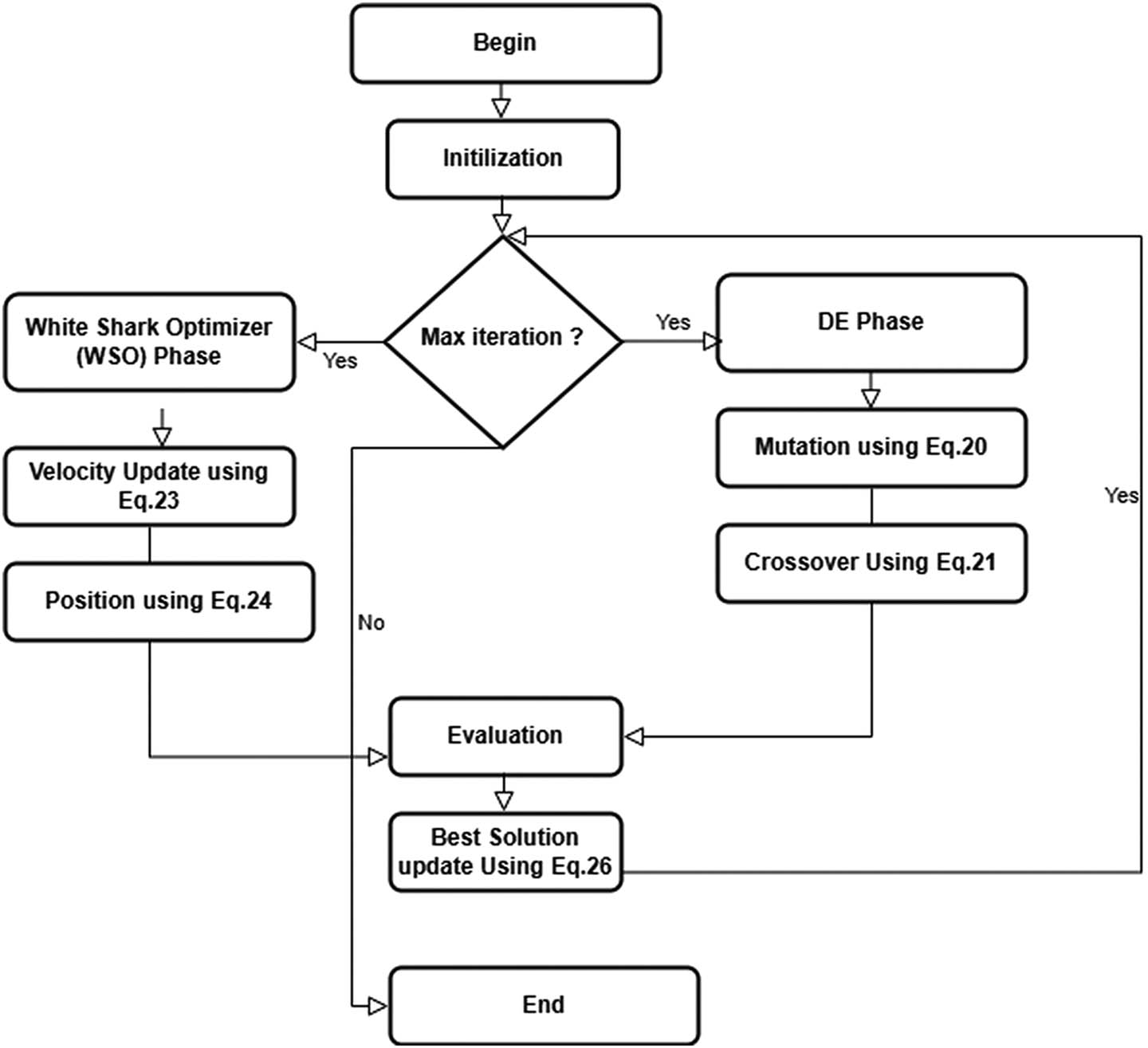
WSODE Flowchart. Source: Created by the authors.
| Algorithm 1. Pseudocode and steps of WSODE algorithm | |
|---|---|
| 1: | Initialization: |
| 2: | Initialize the population randomly within the search space using equation (19) |
| 3: | Differential Evolution (DE) Phase: |
| 4: |
for
|
| 5: |
|
| 6: |
|
| 7: |
|
| 8: |
|
| 9: |
|
| 10: | end for |
| 11: | White Shark Optimizer (WSO) Phase: |
| 12: |
for
|
| 13: |
|
| 14: |
|
| 15: |
|
| 16: |
|
| 17: |
|
| 18: |
|
| 19: | end for |
| 20: | Output: |
| 21: | Return the best solution found and the convergence curve. |
3.2 Exploration, exploitation, and local optima avoidance features of WSODE
WSODE adeptly balances exploration and exploitation through its integration of DE and the WSO. Each phase of the algorithm is tailored to enhance either exploration or exploitation, ensuring a comprehensive search of the solution space and effective refinement of potential solutions.
The exploration capabilities of WSODE are primarily driven by the DE component. DE is renowned for its ability to traverse the search space extensively, preventing the algorithm from getting trapped in local optima. This phase involves the mutation operation, where DE generates mutant vectors by adding the weighted differences between randomly selected population vectors to another vector (equation (20)). The crossover operation combines elements from the target vector and the mutant vector to produce a trial vector (equation (21)). This helps maintain diversity in the population and explores different combinations of solutions. Finally, DE ensures that only the best solutions are carried forward by selecting the better vector between the trial and target vectors (equation (22)). This selection process guarantees that the population evolves towards better solutions.
The exploitation capabilities of WSODE are primarily harnessed through the WSO component, which fine-tunes the solutions obtained from the DE phase. In the WSO phase, the velocity of each individual is updated based on the best positions found so far (equation (23)). The position of each individual is then updated based on its velocity (equation (24)). To ensure that individuals remain within the feasible search space, a boundary check and correction mechanism are employed (equation (25)). The best positions are continually updated based on the fitness values of the solutions, ensuring convergence towards the global optimum (equation (26)). Local optima avoidance is a crucial feature of WSODE. The DE phase introduces diversity through its mutation operation (equation (20)), which consistently generates new solutions from different areas of the search space, reducing the likelihood of the population getting stuck in suboptimal regions. Additionally, the crossover operation (equation (21)) further enhances this diversity by combining different vectors, ensuring the algorithm explores a wide range of solutions.
In the WSO phase, local optima avoidance is enhanced by the use of the velocity updates (equation (31)), which drive individuals toward both global and local best solutions while maintaining a degree of randomness through the weighting factor
3.3 Solving single objective optimization problems using WSODE
WSODE is adept at solving single objective optimization problems, where the goal is to find the best solution that minimizes or maximizes a given objective function. The formulation of the objective function and the step-by-step process of solving such problems using WSODE are outlined below.
A single objective optimization problem can be mathematically formulated as:
where
The algorithm begins by initializing the population randomly within the search space, ensuring a diverse set of initial solutions as described by equation (19). In the DE phase, mutant vectors are generated using equation (20), and trial vectors are created by combining elements from the target and mutant vectors as per equation (21). The better vectors are then selected based on their fitness values, ensuring only the best solutions are carried forward, as formalized by equation (22).
In the WSO phase, the velocities of individuals are updated based on the best positions found so far (equation (23)), and their positions are updated accordingly (equation (24)). A boundary check and correction ensure solutions remain within search space boundaries (equation (25)), and the best solutions are updated based on their fitness values (equation (26)).
The convergence of the optimization process is tracked by recording the best objective function value found up to each iteration using equation (27). The algorithm concludes by returning the best solution found and the convergence curve, indicating the progression of the optimization process.
3.4 Computational complexity analysis of WSODE
The computational complexity of WSODE is analyzed by examining both the DE and WSO phases. Each phase contributes to the overall complexity, which depends on the population size
DE phase complexity: In the DE phase, the algorithm starts by initializing a population of
Mutation involves selecting three random vectors from the population and applying a mutation strategy. This operation takes constant time per individual, i.e.,
Crossover is performed over the
Selection compares the trial and target vectors based on their fitness values, and the better vector is retained for the next generation. The selection step is performed for each individual, and the fitness is evaluated in constant time, i.e.,
The DE phase runs for
WSO phase complexity: After the DE phase, WSO takes over and refines the solutions further. The main operations in the WSO phase include velocity updates, position updates, and fitness evaluations.
Velocity update is performed for each individual by calculating the difference between the current position and the best-known solutions, scaled by a random weighting factor. This operation is performed over all
Position update involves updating each individual’s position based on the velocity and wavy motion. This step also runs over
Fitness evaluation is carried out after updating the positions. The fitness of each individual is evaluated in constant time, i.e.,
The WSO phase runs for
Overall complexity: The total computational complexity of WSODE is the sum of the complexities of both the DE and WSO phases. This is represented as:
Simplifying the expression results in the overall complexity of WSODE
where
4 Data description
4.1 IEEE congress on evolutionary computation CEC2022 benchmark description
The assessment of WSODE efficacy leveraged a comprehensive array of benchmark functions from the CEC2022 competition. These functions are crafted to probe the capabilities and flexibility of evolutionary computation algorithms in diverse optimization environments. The suite includes various types of functions: unimodal, multimodal, hybrid, and composition. Unimodal functions, exemplified by the Shifted and Full Rotated Zakharov function (F1), evaluate the fundamental search capabilities and convergence attributes of the algorithms. In contrast, multimodal functions, such as the Shifted and Full Rotated Levy function (F5), present multiple local optima, thus testing the algorithms’ global search proficiency. Hybrid functions, with Hybrid function 3 (F8) as an instance, integrate aspects of different problem domains to reflect more intricate and practical optimization challenges. Furthermore, composition functions, notably Composition function 4 (F12), combine various problem landscapes into a singular test scenario, assessing the adaptability and resilience of the algorithms.
4.2 IEEE congress on evolutionary computation CEC2021 benchmark description
The CEC2021 benchmark functions are a set of standardized test functions designed to evaluate and compare the performance of optimization algorithms. These functions encompass various types of optimization challenges, including unimodal, multimodal, hybrid, and composition functions, each presenting unique complexities and characteristics. Unimodal functions have a single global optimum, while multimodal functions contain multiple local optima, making them challenging for optimization algorithms to navigate. Hybrid functions combine features from different types of functions, and composition functions blend multiple sub-functions to create highly complex landscapes. The primary goal of these benchmarks is to provide a rigorous and diverse set of problems that can thoroughly test the robustness, efficiency, and accuracy of optimization techniques in a controlled and consistent manner.
4.3 IEEE congress on evolutionary computation CEC2017 benchmark description
The CEC2017 benchmark suite, launched at the IEEE congress on evolutionary computation in 2017, provides a sophisticated array of test functions specifically designed to evaluate and enhance the capabilities of optimization algorithms. This suite is a significant update from previous iterations, incorporating new challenges that accurately reflect the evolving complexities found in real-world optimization scenarios. The suite is systematically organized into different categories including unimodal, multimodal, hybrid, and composition test functions, each tailored to assess distinct aspects of algorithmic performance. Unimodal functions within the suite test the algorithms’ ability to refine solutions in relatively simple environments, focusing on the depth of exploitation required to achieve optimal results. Multimodal functions, by contrast, challenge algorithms on their exploratory capabilities, essential for identifying global optima in landscapes populated with numerous local optima. Hybrid functions examine the versatility of algorithms in handling a mix of these environments, while composition functions are designed to test the algorithms’ proficiency in managing a combination of several complex scenarios concurrently. The design of the CEC2017 functions aims to rigorously evaluate not just the accuracy and speed of algorithms in reaching optimal solutions, but also their robustness, scalability, and adaptability in response to dynamic and noisy environments. This comprehensive testing is crucial for advancing metaheuristic algorithms and other evolutionary computation techniques, ensuring they are sufficiently robust and versatile for practical applications. The CEC2017 benchmark suite thus stands as a vital resource for the optimization community, offering a structured and challenging environment for the continuous evaluation and refinement of algorithms. It plays a pivotal role in driving the innovation and development of advanced optimization methods that are capable of addressing the complex and dynamic challenges present in various sectors.
5 Testing and performance
5.1 Setting parameters for benchmark testing
The setting of parameters is essential for the uniform evaluation of optimization algorithms using the benchmark functions established by the CEC competitions in 2022, 2021, and 2017. These established parameters ensure a standardized environment that facilitates comparative analysis of different evolutionary algorithms. Table 1 provides a summary of these settings across all benchmarks.
Standard parameter configurations for CEC benchmarks
| Parameter | Value |
|---|---|
| Population size | 30 |
| Maximum function evaluations | 1,000 |
| Dimensionality (
|
10 |
| Search range |
|
| Rotation | Included for all rotating functions |
| Shift | Included for all shifting functions |
The chosen population size of 30 and dimensionality of 10 strike an effective balance between computational manageability and the complexity needed for significant testing. A limit of 1,000 function evaluations ensures adequate iterations for the algorithms to demonstrate their potential for convergence, without imposing undue computational demands. The specified search range of
The benchmark functions frequently incorporate rotation and shifting to enhance the complexity, better mimicking real-world optimization scenarios. Excluding noise focuses the results on the algorithms’ ability to adeptly navigate complex environments, rather than dealing with random variations. This structured setting enables an equitable comparison among different algorithms, showcasing their strengths and weaknesses within a broad spectrum of benchmark tests (Table 2).
Detailed parameters for comparative algorithm analysis
| Algorithm | Parameter |
|---|---|
| MFO | Gradually decreases from
|
| SHIO | No additional parameters required |
| FOX | Modularity = 0.01, Exponent = v, Switching likelihood = 0.8 |
| HHO |
|
| WSO | Adjustment constant
|
| DA |
|
| SCA | r1 = random(0, 1), r2 = random(0, 1), r3 = random(0, 1), r4 = random(0,1) |
In conducting a detailed statistical evaluation of various optimization algorithms, we utilized key statistical metrics including the mean, standard deviation (STD). The mean is crucial as it represents the central tendency, summarizing the average results achieved by the algorithms across multiple trials and providing an overview of their general performance levels. The STD is employed to measure the extent of variation or dispersion from the mean, which sheds light on the reliability and uniformity of the results from different tests. These measures are essential for determining the stability and predictability of the algorithms’ effectiveness.
5.2 Discussion of WSODE results on IEEE congress on evolutionary computation CEC 2022 benchmarks
The WSODE algorithm demonstrates outperforming performance across the CEC2022 benchmark suite, designed to evaluate optimization algorithms on complex, high-dimensional, multi-modal, and deceptive landscapes, which present significant challenges for conventional metaheuristics. As shown in Table ??, WSODE consistently outperforms or performs comparably to state-of-the-art algorithms such as WSO, GWO, WOA, MFO, FOX, SHIO, DBO, OHO, SCA, FVIM, and SHO. The results showcase WSODE’s capability to balance exploration and exploitation effectively, which is essential for avoiding premature convergence and achieving high-quality solutions across diverse problem landscapes.
In Function F1, which assesses unimodal performance where algorithms can effectively test their convergence capabilities, WSODE achieves the best performance with a mean value of
For Function F3, which includes deceptive elements to challenge the search strategy, WSODE ranks first with a mean value of
In the highly rugged landscape of Function F6, WSODE secures first place with a mean value of
For the complex multi-modal scenarios in Functions F10 and F11, WSODE achieves first place with mean values of
WSODE comparison results on IEEE congress on evolutionary computation 2022 with FES = 1,000 and 30 independent runs
| Function | Measurments | WSODE | WSO | DE | GWO | WOA | MFO | BOA | SHIO | COA | OHO | SCA | GJO | SHO |
|---|---|---|---|---|---|---|---|---|---|---|---|---|---|---|
| F1 | Mean | 3.00 × 10² | 3.00 × 10² | 4.26 × 10² | 1.07 × 10³ | 1.56 × 10⁴ | 6.66 × 10³ | 7.95 × 10³ | 3.61 × 10³ | 3.34 × 10² | 1.57 × 10⁴ | 1.09 × 10³ | 9.90 × 10² | 1.99 × 10³ |
| Std | 6.56 × 10⁻¹⁴ | 6.11 × 10⁻⁴ | 8.47 × 101 | 1.31 × 10³ | 6.72 × 10³ | 7.21 × 10³ | 2.10 × 10³ | 2.82 × 10³ | 9.73 × 101 | 4.41 × 10³ | 2.40 × 10² | 1.26 × 10³ | 2.61 × 10³ | |
| SEM | 2.08 × 10⁻¹⁴ | 1.93 × 10⁻⁴ | 1.26 × 10² | 4.15 × 10² | 2.12 × 10³ | 2.28 × 10³ | 6.65 × 10² | 8.93 × 10² | 3.08 × 101 | 1.39 × 10³ | 7.60 × 101 | 3.99 × 10² | 8.26 × 10² | |
| Rank | 1 | 2 | 4 | 6 | 12 | 10 | 11 | 9 | 3 | 13 | 7 | 5 | 8 | |
| F2 | Mean | 4.06 × 10 2 | 4.00 × 10² | 4.09 × 10² | 4.24 × 10² | 4.40 × 10² | 4.17 × 10² | 2.07 × 10³ | 4.43 × 10² | 4.13 × 10² | 2.54 × 10³ | 4.53 × 10² | 4.43 × 10² | 4.37 × 10² |
| Std | 3.73 × 1000 | 1.26 × 1000 | 0.00 × 1000 | 3.17 × 101 | 3.58 × 101 | 2.67 × 101 | 9.58 × 10² | 2.84 × 101 | 2.06 × 101 | 9.54 × 10² | 1.29 × 101 | 2.95 × 101 | 3.41 × 101 | |
| SEM | 1.18 × 1000 | 3.99 × 10⁻¹ | 8.92 × 1000 | 1.00 × 101 | 1.13 × 101 | 8.44 × 1000 | 3.03 × 10² | 8.97 × 1000 | 6.51 × 1000 | 3.02 × 10² | 4.07 × 1000 | 9.32 × 1000 | 1.08 × 101 | |
| Rank | 2 | 1 | 3 | 6 | 8 | 5 | 12 | 9 | 4 | 13 | 11 | 10 | 7 | |
| F3 | Mean | 6.00 × 10 2 | 6.00 × 10² | 6.01 × 10² | 6.01 × 10² | 6.30 × 10² | 6.01 × 10² | 6.39 × 10² | 6.05 × 10² | 6.05 × 10² | 6.60 × 10² | 6.19 × 10² | 6.07 × 10² | 6.12 × 10² |
| Std | 8.50 × 10⁻¹¹ | 3.08 × 10⁻¹ | 6.76 × 10⁻¹ | 6.88 × 10⁻¹ | 1.56 × 101 | 4.99 × 10⁻¹ | 5.95 × 1000 | 6.18 × 1000 | 1.36 × 101 | 4.09 × 1000 | 3.88 × 1000 | 7.71 × 1000 | 4.76 × 1000 | |
| SEM | 2.69 × 10⁻¹¹ | 9.75 × 10⁻² | 1.36 × 10⁻¹ | 2.18 × 10⁻¹ | 4.94 × 1000 | 1.58 × 10⁻¹ | 1.88 × 1000 | 1.95 × 1000 | 4.29 × 1000 | 1.29 × 1000 | 1.23 × 1000 | 2.44 × 1000 | 1.50 × 1000 | |
| Rank | 1 | 2 | 4 | 5 | 11 | 3 | 12 | 6 | 7 | 13 | 10 | 8 | 9 | |
| F4 | Mean | 8.16 × 10 2 | 8.08 × 10² | 8.20 × 10² | 8.16 × 10² | 8.42 × 10² | 8.35 × 10² | 8.47 × 10² | 8.16 × 10² | 8.29 × 10² | 8.44 × 10² | 8.41 × 10² | 8.34 × 10² | 8.23 × 10² |
| Std | 7.26 × 1000 | 6.41 × 1000 | 1.35 × 1000 | 3.26 × 1000 | 1.82 × 101 | 1.35 × 101 | 9.93 × 1000 | 4.08 × 1000 | 7.47 × 1000 | 4.03 × 1000 | 6.09 × 1000 | 1.27 × 101 | 8.54 × 1000 | |
| SEM | 2.30 × 1000 | 2.03 × 1000 | 1.96 × 101 | 1.03 × 1000 | 5.77 × 1000 | 4.27 × 1000 | 3.14 × 1000 | 1.29 × 1000 | 2.36 × 1000 | 1.27 × 1000 | 1.93 × 1000 | 4.01 × 1000 | 2.70 × 1000 | |
| Rank | 2 | 1 | 5 | 3 | 11 | 9 | 13 | 4 | 7 | 12 | 10 | 8 | 6 | |
| F5 | Mean | 9.00 × 10 2 | 9.01 × 10² | 9.00 × 10² | 9.06 × 10² | 1.46 × 10³ | 1.03 × 10³ | 1.27 × 10³ | 9.28 × 10² | 9.06 × 10² | 1.57 × 10³ | 1.00 × 10³ | 9.79 × 10² | 1.03 × 10³ |
| Std | 0.00 × 1000 | 8.30 × 10⁻¹ | 1.31 × 10⁻⁵ | 1.10 × 101 | 3.67 × 10² | 2.89 × 10² | 5.85 × 101 | 2.89 × 101 | 8.31 × 1000 | 5.45 × 101 | 3.67 × 101 | 3.10 × 101 | 9.57 × 101 | |
| SEM | 0.00 × 1000 | 2.62 × 10⁻¹ | 7.99 × 10⁻⁶ | 3.48 × 1000 | 1.16 × 10² | 9.13 × 101 | 1.85 × 101 | 9.15 × 1000 | 2.63 × 1000 | 1.72 × 101 | 1.16 × 101 | 9.81 × 1000 | 3.03 × 101 | |
| Rank | 1 | 3 | 2 | 5 | 12 | 10 | 11 | 6 | 4 | 13 | 8 | 7 | 9 | |
| F6 | Mean | 1.80 × 10 3 | 1.81 × 10³ | 2.04 × 10³ | 5.72 × 10³ | 2.80 × 10³ | 5.13 × 10³ | 6.38 × 10⁷ | 4.16 × 10³ | 3.73 × 10³ | 7.30 × 10⁸ | 1.40 × 10⁶ | 8.36 × 10³ | 5.17 × 10³ |
| Std | 4.51 × 10⁻¹ | 4.68 × 1000 | 3.69 × 10² | 2.26 × 10³ | 9.74 × 10² | 2.34 × 10³ | 1.17 × 10⁸ | 2.32 × 10³ | 1.90 × 10³ | 9.77 × 10⁸ | 8.78 × 10⁵ | 2.57 × 10³ | 1.20 × 10³ | |
| SEM | 1.43 × 10⁻¹ | 1.48 × 1000 | 2.35 × 10² | 7.14 × 10² | 3.08 × 10² | 7.40 × 10² | 3.69 × 10⁷ | 7.33 × 10² | 6.02 × 10² | 3.09 × 10⁸ | 2.78 × 10⁵ | 8.12 × 10² | 3.78 × 10² | |
| Rank | 1 | 2 | 3 | 9 | 4 | 7 | 12 | 6 | 5 | 13 | 11 | 10 | 8 | |
| F7 | Mean | 2.01 × 10³ | 2.02 × 10³ | 2.00 × 10³ | 2.03 × 10³ | 2.08 × 10³ | 2.02 × 10³ | 2.08 × 10³ | 2.04 × 10³ | 2.02 × 10³ | 2.13 × 10³ | 2.06 × 10³ | 2.04 × 10³ | 2.03 × 10³ |
| Std | 9.58 × 1000 | 8.67 × 1000 | 5.37 × 10⁻⁵ | 9.85 × 1000 | 2.22 × 101 | 9.14 × 10⁻¹ | 1.33 × 101 | 1.25 × 101 | 8.15 × 1000 | 5.11 × 1000 | 1.34 × 101 | 9.76 × 1000 | 1.12 × 101 | |
| SEM | 3.03 × 1000 | 2.74 × 1000 | 3.59 × 10⁻⁵ | 3.11 × 1000 | 7.02 × 1000 | 2.89 × 10⁻¹ | 4.20 × 1000 | 3.97 × 1000 | 2.58 × 1000 | 1.62 × 1000 | 4.24 × 1000 | 3.09 × 1000 | 3.55 × 1000 | |
| Rank | 2 | 4 | 1 | 6 | 12 | 5 | 11 | 9 | 3 | 13 | 10 | 8 | 7 | |
| F8 | Mean | 2.20 × 10³ | 2.21 × 10³ | 2.20 × 10³ | 2.23 × 10³ | 2.23 × 10³ | 2.22 × 10³ | 2.28 × 10³ | 2.23 × 10³ | 2.22 × 10³ | 2.43 × 10³ | 2.23 × 10³ | 2.23 × 10³ | 2.22 × 10³ |
| Std | 9.80 × 10⁻¹ | 9.49 × 1000 | 2.90 × 1000 | 4.25 × 1000 | 4.28 × 1000 | 4.27 × 1000 | 6.70 × 101 | 3.29 × 1000 | 7.89 × 1000 | 1.27 × 10² | 2.81 × 1000 | 3.50 × 1000 | 1.83 × 1000 | |
| SEM | 3.10 × 10⁻¹ | 3.00 × 1000 | 4.89 × 1000 | 1.34 × 1000 | 1.35 × 1000 | 1.35 × 1000 | 2.12 × 101 | 1.04 × 1000 | 2.50 × 1000 | 4.03 × 101 | 8.88 × 10⁻¹ | 1.11 × 1000 | 5.79 × 10⁻¹ | |
| Rank | 1 | 3 | 2 | 7 | 11 | 6 | 12 | 9 | 4 | 13 | 10 | 8 | 5 | |
| F9 | Mean | 2.53 × 10³ | 2.53 × 10³ | 2.53 × 10³ | 2.56 × 10³ | 2.59 × 10³ | 2.53 × 10³ | 2.76 × 10³ | 2.60 × 10³ | 2.53 × 10³ | 2.84 × 10³ | 2.56 × 10³ | 2.58 × 10³ | 2.59 × 10³ |
| Std | 0.00 × 1000 | 1.48 × 10⁻⁴ | 6.91 × 1000 | 2.85 × 101 | 4.09 × 101 | 6.35 × 1000 | 6.26 × 101 | 3.76 × 101 | 2.11 × 10⁻⁵ | 8.77 × 101 | 1.64 × 101 | 3.06 × 101 | 3.86 × 101 | |
| SEM | 0.00 × 1000 | 4.67 × 10⁻⁵ | 2.33 × 10² | 9.00 × 1000 | 1.29 × 101 | 2.01 × 1000 | 1.98 × 101 | 1.19 × 101 | 6.66 × 10⁻⁶ | 2.77 × 101 | 5.18 × 1000 | 9.68 × 1000 | 1.22 × 101 | |
| Rank | 1 | 3 | 5 | 6 | 9 | 4 | 12 | 11 | 2 | 13 | 7 | 8 | 10 | |
| F10 | Mean | 2.51 × 10³ | 2.54 × 10³ | 2.53 × 10³ | 2.56 × 10³ | 2.54 × 10³ | 2.53 × 10³ | 2.52 × 10³ | 2.53 × 10³ | 2.55 × 10³ | 2.81 × 10³ | 2.52 × 10³ | 2.59 × 10³ | 2.55 × 10³ |
| Std | 3.33 × 101 | 5.57 × 101 | 2.14 × 10⁻² | 5.96 × 101 | 6.97 × 101 | 5.39 × 101 | 4.80 × 101 | 5.39 × 101 | 6.15 × 101 | 2.27 × 10² | 6.25 × 10⁻¹ | 6.03 × 101 | 6.75 × 101 | |
| SEM | 1.05 × 101 | 1.76 × 101 | 1.00 × 10² | 1.88 × 101 | 2.20 × 101 | 1.70 × 101 | 1.52 × 101 | 1.70 × 101 | 1.95 × 101 | 7.17 × 101 | 1.98 × 10⁻¹ | 1.91 × 101 | 2.13 × 101 | |
| Rank | 1 | 7 | 4 | 11 | 8 | 5 | 2 | 6 | 9 | 13 | 3 | 12 | 10 | |
| F11 | Mean | 2.60 × 10³ | 2.65 × 10³ | 2.65 × 10³ | 2.88 × 10³ | 2.78 × 10³ | 2.78 × 10³ | 2.98 × 10³ | 2.82 × 10³ | 2.73 × 10³ | 4.04 × 10³ | 2.82 × 10³ | 2.84 × 10³ | 2.80 × 10³ |
| Std | 4.29 × 10⁻¹³ | 1.01 × 10² | 8.65 × 101 | 2.29 × 10² | 1.31 × 10² | 1.65 × 10² | 1.84 × 10² | 1.84 × 10² | 1.60 × 10² | 3.40 × 10² | 1.46 × 10² | 2.01 × 10² | 2.21 × 10² | |
| SEM | 1.36 × 10⁻¹³ | 3.20 × 101 | 5.05 × 101 | 7.25 × 101 | 4.14 × 101 | 5.22 × 101 | 5.82 × 101 | 5.81 × 101 | 5.07 × 101 | 1.08 × 10² | 4.61 × 101 | 6.36 × 101 | 7.00 × 101 | |
| Rank | 1 | 2 | 3 | 11 | 6 | 5 | 12 | 8 | 4 | 13 | 9 | 10 | 7 | |
| F12 | Mean | 2.86 × 10³ | 2.87 × 10³ | 2.86 × 10³ | 2.87 × 10³ | 2.90 × 10³ | 2.86 × 10³ | 2.92 × 10³ | 2.88 × 10³ | 2.86 × 10³ | 3.21 × 10³ | 2.87 × 10³ | 2.87 × 10³ | 2.88 × 10³ |
| Std | 1.24 × 1000 | 3.74 × 1000 | 1.28 × 1000 | 2.23 × 1000 | 5.89 × 101 | 1.08 × 1000 | 2.88 × 101 | 1.66 × 101 | 2.43 × 1000 | 1.86 × 10² | 1.38 × 1000 | 1.35 × 101 | 1.48 × 101 | |
| SEM | 3.91 × 10⁻¹ | 1.18 × 1000 | 1.64 × 10² | 7.07 × 10⁻¹ | 1.86 × 101 | 3.40 × 10⁻¹ | 9.10 × 1000 | 5.26 × 1000 | 7.68 × 10⁻¹ | 5.89 × 101 | 4.36 × 10⁻¹ | 4.26 × 1000 | 4.69 × 1000 | |
| Rank | 1 | 6 | 4 | 5 | 11 | 2 | 12 | 9 | 3 | 13 | 7 | 8 | 10 |
The Wilcoxon signed-rank test results for the CEC 2022 benchmarks (Table 4) show that the WSODE optimizer demonstrates robust performance across most comparisons. Although WSODE faces challenges from DE, with only 1 win, 5 losses, and 6 ties, it performs better against GWO, achieving 8 wins, 1 loss, and 3 ties. WSODE exhibits dominance over WOA and BOA, winning all 12 functions in both cases without any losses or ties. Similarly, WSODE outperforms MFO with 6 wins, 2 losses, and 4 ties, and shows a strong advantage over SHIO with 11 wins and 1 tie. Against COA, WSODE secures 11 wins and suffers only 1 loss. In flawless comparisons, WSODE wins all functions against OHO (12 wins), SCA (11 wins, 1 tie), and GJO (11 wins, 1 tie). Against SHO, WSODE achieves 10 wins, 1 loss, and 1 tie.
WSODE Wilcoxon signed rank sum (SRS) test results on IEEE congress on evolutionary computation 2022 with FES = 1,000 and 30 independent runs
| Function | WSO | DE | GWO | WOA | MFO | BOA | SHIO | COA | OHO | SCA | GJO | SHO |
|---|---|---|---|---|---|---|---|---|---|---|---|---|
| F1 | 0.557743 | 0.24519 | 0.001114 | 1.73 × 10⁻⁶ | 2.13 × 10⁻⁶ | 1.73 × 10⁻⁶ | 0.000831 | 1.73 × 10⁻⁶ | 1.73 × 10⁻⁶ | 4.73 × 10⁻⁶ | 5.31 × 10⁻⁵ | 0.000115 |
| T+: 261, T-: 204 | T+: 176, T-: 289 | T+: 391, T-: 74 | T+: 465, T-: 0 | T+: 463, T-: 2 | T+: 465, T-: 0 | T+: 395, T-: 70 | T+: 465, T-: 0 | T+: 465, T-: 0 | T+: 455, T-: 10 | T+: 429, T-: 36 | T+: 420, T-: 45 | |
| F2 | 1.13 × 10⁻⁵ | 0.271155 | 8.92 × 10⁻⁵ | 1.73 × 10⁻⁶ | 0.031603 | 1.73 × 10⁻⁶ | 1.73 × 10⁻⁶ | 6.98 × 10⁻⁶ | 1.73 × 10⁻⁶ | 1.73 × 10⁻⁶ | 3.88 × 10⁻⁶ | 2.88 × 10⁻⁶ |
| T+: 446, T-: 19 | T+: 179, T-: 286 | T+: 423, T-: 42 | T+: 465, T-: 0 | T+: 337, T-: 128 | T+: 465, T-: 0 | T+: 465, T-: 0 | T+: 451, T-: 14 | T+: 465, T-: 0 | T+: 465, T-: 0 | T+: 457, T-: 8 | T+: 460, T-: 5 | |
| F3 | 1.73 × 10⁻⁶ | 0.016566 | 0.001709 | 1.73 × 10⁻⁶ | 9.32 × 10⁻⁶ | 1.73 × 10⁻⁶ | 1.73 × 10⁻⁶ | 1.73 × 10⁻⁶ | 1.73 × 10⁻⁶ | 1.73 × 10⁻⁶ | 1.73 × 10⁻⁶ | 1.73 × 10⁻⁶ |
| T+: 465, T-: 0 | T+: 116, T-: 349 | T+: 385, T-: 80 | T+: 465, T-: 0 | T+: 448, T-: 17 | T+: 465, T-: 0 | T+: 465, T-: 0 | T+: 465, T-: 0 | T+: 465, T-: 0 | T+: 465, T-: 0 | T+: 465, T-: 0 | T+: 465, T-: 0 | |
| F4 | 0.000306 | 1.73 × 10⁻⁶ | 0.000174 | 0.001382 | 0.025637 | 1.73 × 10⁻⁶ | 0.813017 | 0.000332 | 1.73 × 10⁻⁶ | 2.88 × 10⁻⁶ | 0.349346 | 5.31 × 10⁻⁵ |
| T+: 408, T-: 57 | T+: 465, T-: 0 | T+: 50, T-: 415 | T+: 388, T-: 77 | T+: 124, T-: 341 | T+: 465, T-: 0 | T+: 244, T-: 221 | T+: 58, T-: 407 | T+: 465, T-: 0 | T+: 460, T-: 5 | T+: 278, T-: 187 | T+: 36, T-: 429 | |
| F5 | 9.32 × 10⁻⁶ | 0.003854 | 0.00016 | 1.73 × 10⁻⁶ | 8.47 × 10⁻⁶ | 1.73 × 10⁻⁶ | 1.73 × 10⁻⁶ | 1.73 × 10⁻⁶ | 1.73 × 10⁻⁶ | 1.73 × 10⁻⁶ | 4.73 × 10⁻⁶ | 1.73 × 10⁻⁶ |
| T+: 448, T-: 17 | T+: 92, T-: 373 | T+: 416, T-: 49 | T+: 465, T-: 0 | T+: 449, T-: 16 | T+: 465, T-: 0 | T+: 465, T-: 0 | T+: 465, T-: 0 | T+: 465, T-: 0 | T+: 465, T-: 0 | T+: 455, T-: 10 | T+: 465, T-: 0 | |
| F6 | 1.24 × 10⁻⁵ | 0.440522 | 1.73 × 10⁻⁶ | 1.73 × 10⁻⁶ | 1.73 × 10⁻⁶ | 1.73 × 10⁻⁶ | 1.73 × 10⁻⁶ | 1.73 × 10⁻⁶ | 1.73 × 10⁻⁶ | 1.73 × 10⁻⁶ | 1.73 × 10⁻⁶ | 1.73 × 10⁻⁶ |
| T+: 445, T-: 20 | T+: 195, T-: 270 | T+: 465, T-: 0 | T+: 465, T-: 0 | T+: 465, T-: 0 | T+: 465, T-: 0 | T+: 465, T-: 0 | T+: 465, T-: 0 | T+: 465, T-: 0 | T+: 465, T-: 0 | T+: 465, T-: 0 | T+: 465, T-: 0 | |
| F7 | 2.88 × 10⁻⁶ | 0.097772 | 0.00439 | 1.92 × 10⁻⁶ | 0.829013 | 1.73 × 10⁻⁶ | 2.6 × 10⁻⁶ | 0.003162 | 1.73 × 10⁻⁶ | 1.73 × 10⁻⁶ | 6.98 × 10⁻⁶ | 2.13 × 10⁻⁶ |
| T+: 460, T-: 5 | T+: 152, T-: 313 | T+: 371, T-: 94 | T+: 464, T-: 1 | T+: 222, T-: 243 | T+: 465, T-: 0 | T+: 461, T-: 4 | T+: 376, T-: 89 | T+: 465, T-: 0 | T+: 465, T-: 0 | T+: 451, T-: 14 | T+: 463, T-: 2 | |
| F8 | 0.007731 | 0.003379 | 0.135908 | 2.6 × 10⁻⁶ | 0.002105 | 1.73 × 10⁻⁶ | 2.84 × 10⁻⁵ | 0.001382 | 1.73 × 10⁻⁶ | 1.92 × 10⁻⁶ | 0.00873 | 0.658331 |
| T+: 362, T-: 103 | T+: 90, T-: 375 | T+: 305, T-: 160 | T+: 461, T-: 4 | T+: 83, T-: 382 | T+: 465, T-: 0 | T+: 436, T-: 29 | T+: 388, T-: 77 | T+: 465, T-: 0 | T+: 464, T-: 1 | T+: 360, T-: 105 | T+: 211, T-: 254 | |
| F9 | 1.73 × 10⁻⁶ | 0.047162 | 2.35 × 10⁻⁶ | 2.13 × 10⁻⁶ | 0.765519 | 1.73 × 10⁻⁶ | 1.73 × 10⁻⁶ | 0.000222 | 1.73 × 10⁻⁶ | 1.73 × 10⁻⁶ | 1.73 × 10⁻⁶ | 1.73 × 10⁻⁶ |
| T+: 465, T-: 0 | T+: 136, T-: 329 | T+: 462, T-: 3 | T+: 463, T-: 2 | T+: 247, T-: 218 | T+: 465, T-: 0 | T+: 465, T-: 0 | T+: 412, T-: 53 | T+: 465, T-: 0 | T+: 465, T-: 0 | T+: 465, T-: 0 | T+: 465, T-: 0 | |
| F10 | 0.016566 | 0.152861 | 0.14139 | 0.002255 | 0.097772 | 0.003379 | 0.000283 | 0.000332 | 1.73 × 10⁻⁶ | 0.059836 | 0.012453 | 4.45 × 10⁻⁵ |
| T+: 349, T-: 116 | T+: 302, T-: 163 | T+: 304, T-: 161 | T+: 381, T-: 84 | T+: 313, T-: 152 | T+: 375, T-: 90 | T+: 409, T-: 56 | T+: 407, T-: 58 | T+: 465, T-: 0 | T+: 324, T-: 141 | T+: 354, T-: 111 | T+: 431, T-: 34 | |
| F11 | 0.075213 | 0.008217 | 0.557743 | 0.000174 | 0.001197 | 2.88 × 10⁻⁶ | 8.19 × 10⁻⁵ | 0.002585 | 1.73 × 10⁻⁶ | 0.00016 | 9.71 × 10⁻⁵ | 0.00049 |
| T+: 319, T-: 146 | T+: 104, T-: 361 | T+: 261, T-: 204 | T+: 415, T-: 50 | T+: 390, T-: 75 | T+: 460, T-: 5 | T+: 424, T-: 41 | T+: 379, T-: 86 | T+: 465, T-: 0 | T+: 416, T-: 49 | T+: 422, T-: 43 | T+: 402, T-: 63 | |
| F12 | 2.13 × 10⁻⁶ | 0.382034 | 0.001709 | 2.35 × 10⁻⁶ | 0.110926 | 1.73 × 10⁻⁶ | 1.92 × 10⁻⁶ | 0.000283 | 1.73 × 10⁻⁶ | 1.49 × 10⁻⁵ | 8.92 × 10⁻⁵ | 1.92 × 10⁻⁶ |
| T+: 463, T-: 2 | T+: 275, T-: 190 | T+: 385, T-: 80 | T+: 462, T-: 3 | T+: 155, T-: 310 | T+: 465, T-: 0 | T+: 464, T-: 1 | T+: 409, T-: 56 | T+: 465, T-: 0 | T+: 443, T-: 22 | T+: 423, T-: 42 | T+: 464, T-: 1 | |
| Total | +:10, -:0, =:2 | +:1, -:5, =:6 | +:8, -:1, =:3 | +:12, -:0, =:0 | +:6, -:2, =:4 | +:12, -:0, =:0 | +:11, -:0, =:1 | +:11, -:1, =:0 | +:12, -:0, =:0 | +:11, -:0, =:1 | +:11, -:0, =:1 | +:10, -:1, =:1 |
5.3 Discussion of the WSODE results on IEEE congress on evolutionary computation CEC 2021
The WSODE algorithm demonstrates significant performance improvements across the CEC2021 benchmark suite, which includes diverse optimization landscapes with varying properties, designed to test algorithms on different aspects such as multi-modality, ruggedness, separability, and deceptive traps. Table 5 presents a detailed comparison of WSODE’s performance against other leading optimizers, including WSO, CMAES, particle swarm optimization (PSO), MVO, DO, MFO, SHIO, SDE, BAT, and FOX, across ten test functions (C1 to C10). These results highlight WSODE’s adaptability and superior ability to navigate complex optimization landscapes.
WSODE comparison results on IEEE congress on evolutionary computation 2021 with FES = 1,000 and 30 independent runs
| Function | WSODE | WSO | CMAES | PSO | MVO | DO | MFO | SHIO | SDE | BAT | FOX | |
|---|---|---|---|---|---|---|---|---|---|---|---|---|
| C1 | Mean | 3.45 × 10⁻³³ | 8.74 × 10⁻⁶ | 2.28 × 10−54 | 9.61 × 10⁻¹⁴ | 6.18 × 10³ | 4.48 × 10⁻³ | 7.00 × 10³ | 1.09 × 10−156 | 1.56 × 10⁻² | 9.20 × 10⁻²² | 1.48 × 10⁻⁸ |
| Std | 1.04 × 10⁻²⁷ | 1.43 × 10⁻⁵ | 4.28 × 10−54 | 1.17 × 10⁻¹³ | 3.99 × 10³ | 4.98 × 10⁻³ | 4.83 × 10³ | 3.38 × 10−156 | 4.95 × 10⁻² | 1.29 × 10−45 | 3.30 × 10⁻⁸ | |
| SEM | 3.28 × 10⁻²⁸ | 4.51 × 10⁻⁶ | 1.35 × 10−54 | 3.72 × 10⁻¹⁴ | 1.26 × 10³ | 1.57 × 10⁻³ | 1.53 × 10³ | 1.07 × 10−156 | 1.56 × 10⁻² | 4.07 × 10−46 | 1.48 × 10⁻⁸ | |
| Rank | 3 | 7 | 2 | 5 | 10 | 8 | 11 | 1 | 9 | 4 | 6 | |
| C2 | Mean | 6.77 × 10 2 | 1.02 × 1000 | 9.13 × 10² | 9.60 × 10² | 6.88 × 10² | 5.50 × 1000 | 9.83 × 10² | 1.78 × 10² | 6.80 × 10² | 7.21 × 10² | 9.81 × 10² |
| Std | 2.33 × 10² | 1.54 × 1000 | 5.90 × 10² | 1.61 × 10² | 3.60 × 10² | 6.21 × 1000 | 2.32 × 10² | 1.83 × 10² | 3.79 × 10² | 1.96 × 10² | 2.19 × 10² | |
| SEM | 7.37 × 101 | 4.88 × 10⁻¹ | 1.87 × 10² | 5.09 × 101 | 1.14 × 10² | 1.96 × 1000 | 7.34 × 101 | 5.78 × 101 | 1.20 × 10² | 6.21 × 101 | 9.81 × 101 | |
| Rank | 4 | 1 | 8 | 9 | 6 | 2 | 11 | 3 | 5 | 7 | 10 | |
| C3 | Mean | 3.06 × 10 1 | 5.73 × 1000 | 3.11 × 101 | 3.26 × 101 | 3.34 × 101 | 5.52 × 1000 | 3.30 × 101 | 3.83 × 101 | 2.51 × 101 | 4.24 × 101 | 3.13 × 101 |
| Std | 2.37 × 1000 | 1.13 × 101 | 8.20 × 1000 | 5.07 × 1000 | 8.01 × 1000 | 8.64 × 1000 | 9.44 × 1000 | 1.55 × 101 | 4.45 × 1000 | 6.60 × 1000 | 1.95 × 1000 | |
| SEM | 7.51 × 10⁻¹ | 3.58 × 1000 | 2.59 × 1000 | 1.60 × 1000 | 2.53 × 1000 | 2.73 × 1000 | 2.98 × 1000 | 4.89 × 1000 | 1.41 × 1000 | 2.09 × 1000 | 8.71 × 10⁻¹ | |
| Rank | 4 | 2 | 5 | 7 | 9 | 1 | 8 | 10 | 3 | 11 | 6 | |
| C4 | Mean | 1.86 × 10 00 | 1.37 × 1000 | 1.93 × 1000 | 1.95 × 1000 | 1.90 × 1000 | 2.97 × 10⁻¹ | 1.89 × 1000 | 1.93 × 1000 | 1.96 × 1000 | 1.93 × 1000 | 1.91 × 1000 |
| Std | 2.34 × 10⁻¹ | 5.32 × 10⁻¹ | 3.02 × 10⁻¹ | 2.35 × 10⁻¹ | 5.66 × 10⁻¹ | 4.02 × 10⁻¹ | 7.09 × 10⁻¹ | 6.64 × 10⁻¹ | 2.90 × 10⁻¹ | 5.69 × 10⁻¹ | 4.90 × 10⁻¹ | |
| SEM | 7.39 × 10⁻² | 1.68 × 10⁻¹ | 9.55 × 10⁻² | 7.44 × 10⁻² | 1.79 × 10⁻¹ | 1.27 × 10⁻¹ | 2.24 × 10⁻¹ | 2.10 × 10⁻¹ | 9.16 × 10⁻² | 1.80 × 10⁻¹ | 2.19 × 10⁻¹ | |
| Rank | 3 | 2 | 7 | 10 | 5 | 1 | 4 | 8 | 11 | 9 | 6 | |
| C5 | Mean | 1.46 × 10 00 | 1.01 × 1000 | 7.23 × 10³ | 3.90 × 10² | 4.22 × 10³ | 4.70 × 1000 | 2.81 × 10² | 3.04 × 1000 | 1.36 × 101 | 2.35 × 101 | 1.24 × 101 |
| Std | 3.54 × 1000 | 4.11 × 10⁻¹ | 5.31 × 10³ | 3.15 × 10² | 2.54 × 10³ | 5.89 × 1000 | 2.51 × 10² | 5.37 × 1000 | 1.39 × 101 | 3.90 × 101 | 5.64 × 1000 | |
| SEM | 1.12 × 1000 | 1.30 × 10⁻¹ | 1.68 × 10³ | 9.96 × 101 | 8.02 × 10² | 1.86 × 1000 | 7.95 × 101 | 1.70 × 1000 | 4.41 × 1000 | 1.23 × 101 | 2.52 × 1000 | |
| Rank | 2 | 1 | 11 | 9 | 10 | 4 | 8 | 3 | 6 | 7 | 5 | |
| C6 | Mean | 3.32 × 10⁻¹ | 7.07 × 10⁻¹ | 4.01 × 101 | 7.09 × 1000 | 4.93 × 101 | 1.21 × 1000 | 2.27 × 101 | 3.42 × 1000 | 1.03 × 101 | 1.10 × 1000 | 8.18 × 1000 |
| Std | 2.96 × 10⁻¹ | 3.83 × 10⁻¹ | 3.13 × 101 | 7.78 × 1000 | 5.42 × 101 | 1.46 × 1000 | 1.48 × 101 | 3.38 × 1000 | 9.73 × 1000 | 5.64 × 10⁻¹ | 9.67 × 1000 | |
| SEM | 9.36 × 10⁻² | 1.21 × 10⁻¹ | 9.89 × 1000 | 2.46 × 1000 | 1.71 × 101 | 4.62 × 10⁻¹ | 4.68 × 1000 | 1.07 × 1000 | 3.08 × 1000 | 1.78 × 10⁻¹ | 4.32 × 1000 | |
| Rank | 1 | 2 | 10 | 6 | 11 | 4 | 9 | 5 | 8 | 3 | 7 | |
| C7 | Mean | 3.36 × 10⁻¹ | 3.94 × 10⁻¹ | 1.96 × 10³ | 1.57 × 10² | 1.45 × 10³ | 4.39 × 1000 | 2.70 × 101 | 5.04 × 10⁻¹ | 1.78 × 1000 | 5.92 × 1000 | 1.78 × 1000 |
| Std | 2.81 × 10⁻¹ | 1.87 × 10⁻¹ | 6.92 × 10² | 2.24 × 10² | 1.23 × 10³ | 1.11 × 101 | 3.82 × 101 | 6.72 × 10⁻¹ | 1.26 × 1000 | 7.88 × 1000 | 6.01 × 10⁻¹ | |
| SEM | 8.88 × 10⁻² | 5.91 × 10⁻² | 2.19 × 10² | 7.09 × 101 | 3.88 × 10² | 3.50 × 1000 | 1.21 × 101 | 2.12 × 10⁻¹ | 3.99 × 10⁻¹ | 2.49 × 1000 | 2.69 × 10⁻¹ | |
| Rank | 1 | 2 | 11 | 9 | 10 | 6 | 8 | 3 | 5 | 7 | 4 | |
| C8 | Mean | 4.07 × 10⁻¹⁶ | 8.98 × 1000 | 6.56 × 1000 | 7.77 × 101 | 5.48 × 10² | 1.22 × 101 | 1.47 × 10² | 1.99 × 101 | 2.57 × 101 | 1.03 × 10² | 4.04 × 101 |
| Std | 5.90 × 10⁻¹⁶ | 7.82 × 1000 | 7.58 × 1000 | 6.95 × 101 | 3.42 × 10² | 3.87 × 101 | 2.52 × 10² | 3.27 × 101 | 1.94 × 101 | 1.60 × 10² | 2.26 × 101 | |
| SEM | 1.87 × 10⁻¹⁶ | 2.47 × 1000 | 2.40 × 1000 | 2.20 × 101 | 1.08 × 10² | 1.22 × 101 | 7.98 × 101 | 1.03 × 101 | 6.13 × 1000 | 5.06 × 101 | 1.01 × 101 | |
| Rank | 1 | 3 | 2 | 8 | 11 | 4 | 10 | 5 | 6 | 9 | 7 | |
| C9 | Mean | 1.60 × 10⁻¹⁴ | 1.41 × 10⁻³ | 3.55 × 10⁻¹⁵ | 3.13 × 10⁻⁹ | 6.47 × 10⁻¹ | 4.53 × 10⁻⁸ | 8.88 × 10⁻¹⁴ | 9.77 × 10⁻¹⁴ | 7.73 × 10⁻¹⁰ | 5.21 × 10⁻¹ | 2.16 × 10⁻¹⁰ |
| Std | 8.16 × 10⁻¹⁵ | 4.40 × 10⁻³ | 4.59 × 10⁻¹⁵ | 4.11 × 10⁻⁹ | 1.39 × 1000 | 2.84 × 10⁻⁸ | 0.00 × 1000 | 2.81 × 10⁻¹⁵ | 8.86 × 10⁻¹⁰ | 1.65 × 1000 | 3.58 × 10⁻¹⁰ | |
| SEM | 2.58 × 10⁻¹⁵ | 1.39 × 10⁻³ | 1.45 × 10⁻¹⁵ | 1.30 × 10⁻⁹ | 4.38 × 10⁻¹ | 8.99 × 10⁻⁹ | 0.00 × 1000 | 8.88 × 10⁻¹⁶ | 2.80 × 10⁻¹⁰ | 5.21 × 10⁻¹ | 1.60 × 10⁻¹⁰ | |
| Rank | 2 | 9 | 1 | 7 | 11 | 8 | 3 | 4 | 6 | 10 | 5 | |
| C10 | Mean | 4.90 × 101 | 4.93 × 101 | 4.92 × 101 | 6.06 × 101 | 4.91 × 101 | 5.19 × 101 | 4.98 × 101 | 5.46 × 101 | 4.91 × 101 | 5.00 × 101 | 4.90 × 101 |
| Std | 2.11 × 10⁻¹ | 7.45 × 10⁻¹ | 1.91 × 10⁻¹ | 1.95 × 101 | 5.48 × 10⁻¹ | 2.16 × 101 | 2.19 × 1000 | 1.03 × 101 | 2.36 × 10⁻¹ | 3.06 × 1000 | 1.90 × 10⁻¹ | |
| SEM | 6.66 × 10⁻² | 2.36 × 10⁻¹ | 6.05 × 10⁻² | 6.18 × 1000 | 1.73 × 10⁻¹ | 6.85 × 1000 | 6.93 × 10⁻¹ | 3.25 × 1000 | 7.47 × 10⁻² | 9.68 × 10⁻¹ | 8.49 × 10⁻² | |
| Rank | 1 | 6 | 5 | 11 | 4 | 9 | 7 | 10 | 3 | 8 | 2 |
Function C1 is a high-dimensional unimodal function, aimed at evaluating an algorithm’s convergence speed and precision in simpler landscapes without local minima. WSODE achieves a mean value of
In Function C2, a unimodal function with added separability, WSODE ranks fourth with a mean value of
Function C3 presents a multi-modal, deceptive landscape, introducing numerous local optima to test an algorithm’s exploration efficiency. WSODE ranks fourth with a mean value of
Function C5 introduces nonseparability and a high degree of variable interaction, challenging algorithms to explore global optima without decomposing the function. WSODE ranks second with a mean value of 1.46 and a STD of 3.54, outperformed only by WSO. This result reflects WSODE’s effective handling of nonseparable problems, outperforming traditional algorithms like CMAES, PSO, and MFO, which tend to struggle with such intricacies.
For Function C6, a deceptive and highly rugged multi-modal function, WSODE ranks first with a mean value of
Function C8, a high-dimensional, multimodal landscape with numerous local optima, poses a challenge for exploitation-dominant algorithms. WSODE achieves the best performance with a mean value of
In Function C9, which introduces deceptive features to test resilience against premature convergence, WSODE ranks second with a mean value of
Finally, Function C10, a nonseparable, high-dimensional problem with deceptive traps and ruggedness, represents one of the most challenging functions in the CEC2021 suite. WSODE ranks first with a mean value of
As shown in Table 6, the Wilcoxon signed-rank test results demonstrate that the WSODE optimizer consistently achieves significant performance advantages over other optimizers on the CEC 2021 benchmark set. WSODE secures a majority of significant wins across comparisons, achieving flawless or near-flawless results against several algorithms, including WOA, BOA, and OHO, with no losses. While WSODE demonstrates robustness across all comparisons, it encounters minimal challenges from GWO and MFO, which manage to achieve a single loss and several ties, respectively.
WSODE Wilcoxon Signed rank results on IEEE Congress on Evolutionary Computation 2021 with FES = 1,000 and 30 independent runs
| Function | WSO | CSAES | PSO | MVO | DO | MFO | SHIO | SDE | BAT | FOX |
|---|---|---|---|---|---|---|---|---|---|---|
| F1 | 0.478125 | 0.001713 | 8.86 × 10⁻⁵ | 8.86 × 10⁻⁵ | 8.86 × 10⁻⁵ | 0.001507 | 0.000103 | 8.86 × 10⁻⁵ | 0.000189 | 0.00078 |
| T+: 124, T−: 86 | T+: 189, T−: 21 | T+: 210, T−: 0 | T+: 210, T−: 0 | T+: 210, T−: 0 | T+: 190, T−: 20 | T+: 209, T−: 1 | T+: 210, T−: 0 | T+: 205, T−: 5 | T+: 195, T−: 15 | |
| F2 | 0.002821 | 8.86 × 10⁻⁵ | 8.86 × 10⁻⁵ | 0.079322 | 8.86 × 10⁻⁵ | 0.000189 | 0.005734 | 8.86 × 10⁻⁵ | 8.86 × 10⁻⁵ | 0.000103 |
| T+: 185, T−: 25 | T+: 210, T−: 0 | T+: 210, T−: 0 | T+: 152, T−: 58 | T+: 210, T−: 0 | T+: 205, T−: 5 | T+: 179, T−: 31 | T+: 210, T−: 0 | T+: 210, T−: 0 | T+: 209, T−: 1 | |
| F3 | 8.86 × 10⁻⁵ | 8.86 × 10⁻⁵ | 8.86 × 10⁻⁵ | 0.000103 | 8.86 × 10⁻⁵ | 8.86 × 10⁻⁵ | 0.000103 | 8.86 × 10⁻⁵ | 8.86 × 10⁻⁵ | 8.86 × 10⁻⁵ |
| T+: 210, T−: 0 | T+: 210, T−: 0 | T+: 210, T−: 0 | T+: 209, T−: 1 | T+: 210, T−: 0 | T+: 210, T−: 0 | T+: 209, T−: 1 | T+: 210, T−: 0 | T+: 210, T−: 0 | T+: 210, T−: 0 | |
| F4 | 0.411465 | 0.006425 | 0.00014 | 0.601213 | 8.86 × 10⁻⁵ | 0.575486 | 0.262722 | 8.86 × 10⁻⁵ | 0.000103 | 0.295878 |
| T+: 127, T−: 83 | T+: 32, T−: 178 | T+: 207, T−: 3 | T+: 119, T−: 91 | T+: 210, T−: 0 | T+: 90, T−: 120 | T+: 135, T−: 75 | T+: 210, T−: 0 | T+: 209, T−: 1 | T+: 133, T−: 77 | |
| F5 | 8.86 × 10⁻⁵ | 8.86 × 10⁻⁵ | 8.86 × 10⁻⁵ | 0.000103 | 8.86 × 10⁻⁵ | 8.86 × 10⁻⁵ | 8.86 × 10⁻⁵ | 8.86 × 10⁻⁵ | 8.86 × 10⁻⁵ | 8.86 × 10⁻⁵ |
| T+: 210, T−: 0 | T+: 210, T−: 0 | T+: 210, T−: 0 | T+: 209, T−: 1 | T+: 210, T−: 0 | T+: 210, T−: 0 | T+: 210, T−: 0 | T+: 210, T−: 0 | T+: 210, T−: 0 | T+: 210, T−: 0 | |
| F6 | 0.156004 | 8.86 × 10⁻⁵ | 8.86 × 10⁻⁵ | 8.86 × 10⁻⁵ | 8.86 × 10⁻⁵ | 8.86 × 10⁻⁵ | 8.86 × 10⁻⁵ | 8.86 × 10⁻⁵ | 8.86 × 10⁻⁵ | 8.86 × 10⁻⁵ |
| T+: 143, T−: 67 | T+: 210, T−: 0 | T+: 210, T−: 0 | T+: 210, T−: 0 | T+: 210, T−: 0 | T+: 210, T−: 0 | T+: 210, T−: 0 | T+: 210, T−: 0 | T+: 210, T−: 0 | T+: 210, T−: 0 | |
| F7 | 0.000681 | 0.00014 | 8.86 × 10⁻⁵ | 0.167184 | 8.86 × 10⁻⁵ | 8.86 × 10⁻⁵ | 0.156004 | 8.86 × 10⁻⁵ | 8.86 × 10⁻⁵ | 0.00014 |
| T+: 196, T−: 14 | T+: 207, T−: 3 | T+: 210, T−: 0 | T+: 142, T−: 68 | T+: 210, T−: 0 | T+: 210, T−: 0 | T+: 143, T−: 67 | T+: 210, T−: 0 | T+: 210, T−: 0 | T+: 207, T−: 3 | |
| F8 | 0.001507 | 0.108427 | 8.86 × 10⁻⁵ | 0.881293 | 8.86 × 10⁻⁵ | 8.86 × 10⁻⁵ | 0.000593 | 8.86 × 10⁻⁵ | 8.86 × 10⁻⁵ | 0.000681 |
| T+: 190, T−: 20 | T+: 148, T−: 62 | T+: 210, T−: 0 | T+: 101, T−: 109 | T+: 210, T−: 0 | T+: 210, T−: 0 | T+: 197, T−: 13 | T+: 210, T−: 0 | T+: 210, T−: 0 | T+: 196, T−: 14 | |
| F9 | 8.86 × 10⁻⁵ | 8.86 × 10⁻⁵ | 8.86 × 10⁻⁵ | 0.007189 | 8.86 × 10⁻⁵ | 8.86 × 10⁻⁵ | 0.001019 | 8.86 × 10⁻⁵ | 8.86 × 10⁻⁵ | 8.86 × 10⁻⁵ |
| T+: 210, T−: 0 | T+: 210, T−: 0 | T+: 210, T−: 0 | T+: 177, T−: 33 | T+: 210, T−: 0 | T+: 210, T−: 0 | T+: 193, T−: 17 | T+: 210, T−: 0 | T+: 210, T−: 0 | T+: 210, T−: 0 | |
| F10 | 0.217957 | 0.167184 | 0.002495 | 0.125859 | 0.601213 | 0.002821 | 0.331723 | 0.000103 | 0.135357 | 0.000681 |
| T+: 138, T−: 72 | T+: 142, T−: 68 | T+: 186, T−: 24 | T+: 146, T−: 64 | T+: 91, T−: 119 | T+: 185, T−: 25 | T+: 131, T−: 79 | T+: 209, T−: 1 | T+: 145, T−: 65 | T+: 196, T−: 14 | |
| Total | +:6, −:0, =:4 | +:7, −:1, =:2 | +:10, −:0, =:0 | +:5, −:0, =:5 | +:9, −:0, =:1 | +:9, −:0, =:1 | +:7, −:0, =:3 | +:10, −:0, =:0 | +:9, −:0, =:1 | +:9, −:0, =:1 |
5.4 WSODE comparison results on IEEE congress on evolutionary computation 2017
The performance of WSODE was evaluated against several prominent optimizers, including WSO, CMAES, COA, RSA, BBO, AVOA, SDE, SCA, WOA, DO, MFO, SHIO, and AOA, on the benchmark functions provided by the IEEE CEC 2017 competition (F1–F15). As detailed in Table 7, WSODE exhibits superior performance across a majority of the tested functions, achieving the lowest mean values in numerous cases, which underscores its high optimization efficacy.
WSODE comparison results on IEEE congress on evolutionary computation 2017 (F1–F15) with FES = 1,000 and 30 independent runs
| Function | Statistics | WSODE | WSO | DE | CMAES | COA | RSA | BBO | AVOA | SDE | SCA | WOA | DO | MFO | SHIO | AOA |
|---|---|---|---|---|---|---|---|---|---|---|---|---|---|---|---|---|
| F1 | Mean | 1.00 × 10² | 1.20 × 10² | 1.14 × 10² | 4.44 × 10⁹ | 4.01 × 10³ | 1.54 × 10¹⁰ | 3.25 × 10⁹ | 6.10 × 10⁹ | 5.19 × 10⁹ | 8.16 × 10⁸ | 6.97 × 10⁵ | 3.65 × 10³ | 1.17 × 10⁷ | 6.81 × 10⁷ | 1.61 × 10¹⁰ |
| Std | 8.99 × 10⁻¹⁵ | 4.50 × 101 | 2.49 × 101 | 1.25 × 10⁹ | 1.74 × 10³ | 3.01 × 10⁹ | 7.52 × 10⁸ | 2.81 × 10⁹ | 3.46 × 10⁹ | 2.48 × 10⁸ | 5.02 × 10⁵ | 3.23 × 10³ | 2.86 × 10⁷ | 1.58 × 10⁸ | 3.37 × 10⁹ | |
| SEM | 3.67 × 10⁻¹⁵ | 1.84 × 101 | 1.44 × 101 | 5.10 × 10⁸ | 7.09 × 10² | 1.35 × 10⁹ | 3.36 × 10⁸ | 1.26 × 10⁹ | 1.55 × 10⁹ | 1.01 × 10⁸ | 2.05 × 10⁵ | 1.32 × 10³ | 1.17 × 10⁷ | 6.47 × 10⁷ | 1.51 × 10⁹ | |
| Rank | 1 | 3 | 2 | 11 | 5 | 14 | 10 | 13 | 12 | 9 | 6 | 4 | 7 | 8 | 15 | |
| F2 | Mean | 2.00 × 10 2 | 2.00 × 10² | 2.01 × 10² | 2.83 × 10¹¹ | 2.00 × 10² | 1.08 × 10¹³ | 1.39 × 10¹¹ | 1.24 × 10¹¹ | 1.78 × 10¹¹ | 5.22 × 10⁷ | 2.55 × 10⁴ | 2.00 × 10² | 5.37 × 10⁷ | 1.33 × 10⁷ | 2.96 × 10¹³ |
| Std | 8.84 × 10⁻¹⁰ | 4.25 × 10⁻⁶ | 2.42 × 1000 | 2.44 × 10¹¹ | 1.38 × 10⁻³ | 1.27 × 10¹³ | 2.26 × 10¹¹ | 1.69 × 10¹¹ | 2.28 × 10¹¹ | 4.40 × 10⁷ | 2.15 × 10⁴ | 2.48 × 10⁻³ | 1.27 × 10⁸ | 2.06 × 10⁷ | 4.21 × 10¹³ | |
| SEM | 3.61 × 10⁻¹⁰ | 1.73 × 10⁻⁶ | 1.40 × 1000 | 9.98 × 10¹⁰ | 5.62 × 10⁻⁴ | 5.68 × 10¹² | 1.01 × 10¹¹ | 7.55 × 10¹⁰ | 1.02 × 10¹¹ | 1.80 × 10⁷ | 8.77 × 10³ | 1.01 × 10⁻³ | 5.17 × 10⁷ | 8.40 × 10⁶ | 1.88 × 10¹³ | |
| Rank | 1 | 2 | 5 | 13 | 3 | 14 | 11 | 10 | 12 | 8 | 6 | 4 | 9 | 7 | 15 | |
| F3 | Mean | 3.00 × 10 2 | 3.00 × 10² | 4.03 × 10² | 3.42 × 10⁴ | 3.03 × 10² | 1.70 × 10⁴ | 3.59 × 10⁴ | 4.21 × 10⁴ | 2.58 × 10⁴ | 1.51 × 10³ | 1.26 × 10³ | 3.00 × 10² | 2.42 × 10³ | 5.81 × 10³ | 3.94 × 10⁴ |
| Std | 2.54 × 10⁻¹⁴ | 8.62 × 10⁻² | 4.23 × 101 | 1.23 × 10⁴ | 3.58 × 1000 | 2.33 × 10³ | 7.81 × 10³ | 2.12 × 10⁴ | 6.12 × 10³ | 6.53 × 10² | 6.48 × 10² | 4.27 × 10⁻³ | 4.22 × 10³ | 3.95 × 10³ | 2.69 × 10⁴ | |
| SEM | 1.04 × 10⁻¹⁴ | 3.52 × 10⁻² | 1.03 × 10² | 5.01 × 10³ | 1.46 × 1000 | 1.04 × 10³ | 3.49 × 10³ | 9.48 × 10³ | 2.74 × 10³ | 2.67 × 10² | 2.64 × 10² | 1.74 × 10⁻³ | 1.72 × 10³ | 1.61 × 10³ | 1.20 × 10⁴ | |
| Rank | 1 | 3 | 5 | 12 | 4 | 10 | 13 | 15 | 11 | 7 | 6 | 2 | 8 | 9 | 14 | |
| F4 | Mean | 4.01 × 10 2 | 4.02 × 10² | 4.06 × 10² | 6.08 × 10² | 4.04 × 10² | 1.86 × 10³ | 6.07 × 10² | 9.49 × 10² | 9.50 × 10² | 4.36 × 10² | 4.27 × 10² | 4.05 × 10² | 4.29 × 10² | 4.19 × 10² | 1.41 × 10³ |
| Std | 5.60 × 10⁻¹ | 1.55 × 1000 | 6.81 × 10⁻¹ | 1.22 × 10² | 1.30 × 1000 | 3.67 × 10² | 7.56 × 101 | 3.71 × 10² | 1.65 × 10² | 3.37 × 1000 | 4.24 × 101 | 7.43 × 10⁻¹ | 2.77 × 101 | 3.01 × 101 | 4.69 × 10² | |
| SEM | 2.29 × 10⁻¹ | 6.31 × 10⁻¹ | 6.18 × 1000 | 4.99 × 101 | 5.31 × 10⁻¹ | 1.64 × 10² | 3.38 × 101 | 1.66 × 10² | 7.36 × 101 | 1.38 × 1000 | 1.73 × 101 | 3.03 × 10⁻¹ | 1.13 × 101 | 1.23 × 101 | 2.10 × 10² | |
| Rank | 1 | 2 | 5 | 11 | 3 | 15 | 10 | 12 | 13 | 9 | 7 | 4 | 8 | 6 | 14 | |
| F5 | Mean | 5.15 × 10 2 | 5.11 × 10² | 5.11 × 10² | 5.68 × 10² | 5.15 × 10² | 6.36 × 10² | 5.71 × 10² | 6.02 × 10² | 6.06 × 10² | 5.47 × 10² | 5.56 × 10² | 5.34 × 10² | 5.31 × 10² | 5.28 × 10² | 6.21 × 10² |
| Std | 9.27 × 1000 | 7.32 × 1000 | 2.03 × 1000 | 1.82 × 101 | 8.85 × 1000 | 2.01 × 101 | 4.36 × 1000 | 2.16 × 101 | 1.29 × 101 | 9.57 × 1000 | 9.63 × 1000 | 1.25 × 101 | 2.10 × 101 | 7.67 × 1000 | 1.48 × 101 | |
| SEM | 3.79 × 1000 | 2.99 × 1000 | 1.07 × 101 | 7.44 × 1000 | 3.61 × 1000 | 8.98 × 1000 | 1.95 × 1000 | 9.66 × 1000 | 5.76 × 1000 | 3.91 × 1000 | 3.93 × 1000 | 5.10 × 1000 | 8.56 × 1000 | 3.13 × 1000 | 6.62 × 1000 | |
| Rank | 3 | 2 | 1 | 10 | 4 | 15 | 11 | 12 | 13 | 8 | 9 | 7 | 6 | 5 | 14 | |
| F6 | Mean | 6.00 × 10 2 | 6.01 × 10² | 6.01 × 10² | 6.30 × 10² | 6.03 × 10² | 6.65 × 10² | 6.38 × 10² | 6.47 × 10² | 6.46 × 10² | 6.15 × 10² | 6.42 × 10² | 6.07 × 10² | 6.01 × 10² | 6.04 × 10² | 6.62 × 10² |
| Std | 1.66 × 10⁻¹⁰ | 7.60 × 10⁻¹ | 1.05 × 101 | 2.92 × 101 | 6.70 × 1000 | 1.03 × 101 | 1.12 × 101 | 1.78 × 101 | 1.56 × 101 | 3.99 × 1000 | 1.25 × 101 | 6.59 × 1000 | 5.68 × 10⁻¹ | 4.82 × 1000 | 6.06 × 1000 | |
| SEM | 6.78 × 10⁻¹¹ | 3.10 × 10⁻¹ | 1.11 × 101 | 1.19 × 101 | 2.74 × 1000 | 4.62 × 1000 | 5.02 × 1000 | 7.98 × 1000 | 6.96 × 1000 | 1.63 × 1000 | 5.11 × 1000 | 2.69 × 1000 | 2.32 × 10⁻¹ | 1.97 × 1000 | 2.71 × 1000 | |
| Rank | 1 | 3 | 3 | 9 | 5 | 15 | 10 | 13 | 12 | 8 | 11 | 7 | 2 | 6 | 14 | |
| F7 | Mean | 7.28 × 10 2 | 7.24 × 10² | 7.32 × 10² | 7.34 × 10² | 7.62 × 10² | 8.26 × 10² | 8.59 × 10² | 8.69 × 10² | 8.59 × 10² | 7.71 × 10² | 7.83 × 10² | 7.51 × 10² | 7.41 × 10² | 7.39 × 10² | 8.78 × 10² |
| Std | 5.34 × 1000 | 9.55 × 10⁻¹ | 5.43 × 1000 | 3.84 × 1000 | 2.05 × 101 | 1.32 × 101 | 2.09 × 101 | 2.91 × 101 | 3.36 × 101 | 9.68 × 1000 | 2.95 × 101 | 1.26 × 101 | 2.09 × 101 | 1.73 × 101 | 2.71 × 101 | |
| SEM | 2.18 × 1000 | 3.90 × 10⁻¹ | 2.22 × 101 | 1.57 × 1000 | 8.38 × 1000 | 5.88 × 1000 | 9.36 × 1000 | 1.30 × 101 | 1.50 × 101 | 3.95 × 1000 | 1.21 × 101 | 5.16 × 1000 | 8.51 × 1000 | 7.07 × 1000 | 1.21 × 101 | |
| Rank | 2 | 1 | 3 | 4 | 8 | 11 | 13 | 14 | 12 | 9 | 10 | 7 | 6 | 5 | 15 | |
| F8 | Mean | 8.09 × 10² | 8.05 × 10² | 8.11 × 10² | 8.19 × 10² | 8.23 × 10² | 8.77 × 10² | 8.74 × 10² | 8.85 × 10² | 8.84 × 10² | 8.39 × 10² | 8.26 × 10² | 8.26 × 10² | 8.25 × 10² | 8.23 × 10² | 8.90 × 10² |
| Std | 8.79 × 1000 | 1.16 × 1000 | 2.06 × 1000 | 9.06 × 1000 | 7.69 × 1000 | 1.07 × 101 | 4.89 × 1000 | 9.47 × 1000 | 1.57 × 101 | 8.91 × 1000 | 1.06 × 101 | 9.13 × 1000 | 7.23 × 1000 | 1.05 × 101 | 2.25 × 101 | |
| SEM | 3.59 × 1000 | 4.73 × 10⁻¹ | 1.06 × 101 | 3.70 × 1000 | 3.14 × 1000 | 4.80 × 1000 | 2.19 × 1000 | 4.23 × 1000 | 7.00 × 1000 | 3.64 × 1000 | 4.33 × 1000 | 3.73 × 1000 | 2.95 × 1000 | 4.27 × 1000 | 1.01 × 101 | |
| Rank | 2 | 1 | 3 | 4 | 6 | 12 | 11 | 14 | 13 | 10 | 9 | 8 | 7 | 5 | 15 | |
| F9 | Mean | 9.00 × 10² | 9.01 × 10² | 9.00 × 10² | 9.00 × 10² | 9.02 × 10² | 2.25 × 10³ | 1.77 × 10³ | 2.42 × 10³ | 1.97 × 10³ | 9.98 × 10² | 1.14 × 10³ | 9.00 × 10² | 9.31 × 10² | 1.09 × 10³ | 2.53 × 10³ |
| Std | 0.00 × 1000 | 1.37 × 1000 | 0.00 × 1000 | 0.00 × 1000 | 3.59 × 1000 | 5.61 × 10² | 4.40 × 10² | 1.36 × 10³ | 2.73 × 10² | 5.30 × 101 | 2.28 × 10² | 1.82 × 10⁻¹ | 6.84 × 101 | 2.31 × 10² | 1.17 × 10³ | |
| SEM | 0.00 × 1000 | 5.60 × 10⁻¹ | 0.00 × 1000 | 0.00 × 1000 | 1.47 × 1000 | 2.51 × 10² | 1.97 × 10² | 6.07 × 10² | 1.22 × 10² | 2.16 × 101 | 9.31 × 101 | 7.42 × 10⁻² | 2.79 × 101 | 9.41 × 101 | 5.25 × 10² | |
| Rank | 1 | 5 | 1 | 1 | 6 | 13 | 11 | 14 | 12 | 8 | 10 | 4 | 7 | 9 | 15 | |
| F10 | Mean | 1.93 × 10³ | 1.58 × 10³ | 1.68 × 10³ | 2.68 × 10³ | 1.73 × 10³ | 3.45 × 10³ | 3.32 × 10³ | 3.05 × 10³ | 3.20 × 10³ | 2.36 × 10³ | 2.11 × 10³ | 1.78 × 10³ | 1.77 × 10³ | 2.05 × 10³ | 3.36 × 10³ |
| Std | 3.23 × 10² | 4.01 × 10² | 1.45 × 10² | 2.47 × 10² | 1.78 × 10² | 2.00 × 10² | 3.04 × 10² | 3.05 × 10² | 2.41 × 10² | 1.85 × 10² | 5.53 × 10² | 2.75 × 10² | 3.60 × 10² | 2.64 × 10² | 3.41 × 10² | |
| SEM | 1.32 × 10² | 1.64 × 10² | 5.80 × 10² | 1.01 × 10² | 7.28 × 101 | 8.95 × 101 | 1.36 × 10² | 1.36 × 10² | 1.08 × 10² | 7.53 × 101 | 2.26 × 10² | 1.12 × 10² | 1.47 × 10² | 1.08 × 10² | 1.52 × 10² | |
| Rank | 6 | 1 | 2 | 10 | 3 | 15 | 13 | 11 | 12 | 9 | 8 | 5 | 4 | 7 | 14 | |
| F11 | Mean | 1.10 × 10³ | 1.11 × 10³ | 1.10 × 10³ | 1.44 × 10³ | 1.18 × 10³ | 1.52 × 10⁴ | 2.53 × 10³ | 4.30 × 10³ | 2.36 × 10³ | 1.21 × 10³ | 1.18 × 10³ | 1.13 × 10³ | 1.17 × 10³ | 1.17 × 10³ | 5.85 × 10³ |
| Std | 5.47 × 10⁻¹ | 6.33 × 1000 | 1.48 × 1000 | 3.08 × 10² | 8.08 × 101 | 1.45 × 10⁴ | 8.30 × 10² | 2.05 × 10³ | 8.93 × 10² | 2.40 × 101 | 3.83 × 101 | 1.23 × 101 | 1.17 × 10² | 2.87 × 101 | 1.48 × 10³ | |
| SEM | 2.23 × 10⁻¹ | 2.58 × 1000 | 2.55 × 1000 | 1.26 × 10² | 3.30 × 101 | 6.50 × 10³ | 3.71 × 10² | 9.17 × 10² | 3.99 × 10² | 9.81 × 1000 | 1.56 × 101 | 5.01 × 1000 | 4.76 × 101 | 1.17 × 101 | 6.62 × 10² | |
| Rank | 1 | 3 | 2 | 10 | 7 | 15 | 12 | 13 | 11 | 9 | 8 | 4 | 5 | 6 | 14 | |
| F12 | Mean | 1.25 × 10³ | 1.64 × 10³ | 1.60 × 10⁴ | 1.07 × 10⁸ | 1.74 × 10⁴ | 2.84 × 10⁸ | 2.31 × 10⁸ | 3.89 × 10⁸ | 1.47 × 10⁸ | 8.19 × 10⁶ | 5.10 × 10⁶ | 2.40 × 10⁵ | 2.75 × 10⁶ | 5.06 × 10⁵ | 1.31 × 10⁹ |
| Std | 6.96 × 101 | 1.37 × 10² | 2.07 × 10³ | 8.48 × 10⁷ | 2.10 × 10⁴ | 2.09 × 10⁸ | 1.13 × 10⁸ | 2.42 × 10⁸ | 6.52 × 10⁷ | 4.26 × 10⁶ | 6.64 × 10⁶ | 2.95 × 10⁵ | 4.23 × 10⁶ | 4.56 × 10⁵ | 5.28 × 10⁸ | |
| SEM | 2.84 × 101 | 5.60 × 101 | 1.48 × 10⁴ | 3.46 × 10⁷ | 8.55 × 10³ | 9.33 × 10⁷ | 5.05 × 10⁷ | 1.08 × 10⁸ | 2.92 × 10⁷ | 1.74 × 10⁶ | 2.71 × 10⁶ | 1.20 × 10⁵ | 1.73 × 10⁶ | 1.86 × 10⁵ | 2.36 × 10⁸ | |
| Rank | 1 | 2 | 3 | 10 | 4 | 13 | 12 | 14 | 11 | 9 | 8 | 5 | 7 | 6 | 15 | |
| F13 | Mean | 1.30 × 10³ | 1.32 × 10³ | 1.31 × 10³ | 4.64 × 10⁵ | 4.37 × 10³ | 4.91 × 10⁷ | 5.68 × 10⁶ | 8.95 × 10⁵ | 7.25 × 10⁶ | 3.27 × 10⁴ | 2.03 × 10⁴ | 1.03 × 10⁴ | 1.33 × 10⁴ | 1.15 × 10⁴ | 1.05 × 10⁸ |
| Std | 1.74 × 1000 | 5.97 × 1000 | 1.88 × 1000 | 1.04 × 10⁶ | 2.60 × 10³ | 3.56 × 10⁷ | 7.37 × 10⁶ | 9.03 × 10⁵ | 7.69 × 10⁶ | 2.28 × 10⁴ | 1.67 × 10⁴ | 9.22 × 10³ | 1.22 × 10⁴ | 6.30 × 10³ | 1.18 × 10⁸ | |
| SEM | 7.12 × 10⁻¹ | 2.44 × 1000 | 9.61 × 1000 | 4.25 × 10⁵ | 1.06 × 10³ | 1.59 × 10⁷ | 3.29 × 10⁶ | 4.04 × 10⁵ | 3.44 × 10⁶ | 9.32 × 10³ | 6.81 × 10³ | 3.76 × 10³ | 5.00 × 10³ | 2.57 × 10³ | 5.26 × 10⁷ | |
| Rank | 1 | 3 | 2 | 10 | 4 | 14 | 12 | 11 | 13 | 9 | 8 | 5 | 7 | 6 | 15 | |
| F14 | Mean | 1.40 × 10³ | 1.42 × 10³ | 1.40 × 10³ | 4.73 × 10³ | 1.56 × 10³ | 3.22 × 10⁵ | 2.66 × 10⁴ | 8.05 × 10³ | 4.39 × 10⁴ | 1.63 × 10³ | 2.26 × 10³ | 1.52 × 10³ | 2.65 × 10³ | 2.78 × 10³ | 5.90 × 10⁵ |
| Std | 7.89 × 1000 | 2.09 × 1000 | 6.06 × 10⁻¹ | 2.33 × 10³ | 9.17 × 101 | 3.40 × 10⁵ | 2.41 × 10⁴ | 5.82 × 10³ | 4.99 × 10⁴ | 1.45 × 10² | 1.45 × 10³ | 1.31 × 10² | 5.18 × 10² | 1.91 × 10³ | 6.84 × 10⁵ | |
| SEM | 3.22 × 1000 | 8.52 × 10⁻¹ | 4.81 × 10⁻¹ | 9.53 × 10² | 3.74 × 101 | 1.52 × 10⁵ | 1.08 × 10⁴ | 2.60 × 10³ | 2.23 × 10⁴ | 5.90 × 101 | 5.91 × 10² | 5.34 × 101 | 2.11 × 10² | 7.80 × 10² | 3.06 × 10⁵ | |
| Rank | 1 | 3 | 2 | 10 | 5 | 14 | 12 | 11 | 13 | 6 | 7 | 4 | 8 | 9 | 15 | |
| F15 | Mean | 1.50 × 10³ | 1.51 × 10³ | 1.50 × 10³ | 4.42 × 10³ | 1.96 × 10³ | 9.26 × 10⁴ | 6.29 × 10⁴ | 1.98 × 10⁴ | 4.17 × 10⁵ | 2.30 × 10³ | 6.52 × 10³ | 2.25 × 10³ | 4.06 × 10³ | 6.26 × 10³ | 3.18 × 10⁶ |
| Std | 2.43 × 10⁻¹ | 1.37 × 101 | 3.28 × 10⁻¹ | 8.64 × 10² | 4.07 × 10² | 1.01 × 10⁵ | 6.11 × 10⁴ | 9.49 × 10³ | 6.20 × 10⁵ | 7.66 × 10² | 3.24 × 10³ | 1.36 × 10³ | 2.27 × 10³ | 8.60 × 10³ | 4.77 × 10⁶ | |
| SEM | 9.90 × 10⁻² | 5.59 × 1000 | 9.72 × 10⁻¹ | 3.53 × 10² | 1.66 × 10² | 4.53 × 10⁴ | 2.73 × 10⁴ | 4.24 × 10³ | 2.77 × 10⁵ | 3.13 × 10² | 1.32 × 10³ | 5.56 × 10² | 9.28 × 10² | 3.51 × 10³ | 2.13 × 10⁶ | |
| Rank | 1 | 3 | 2 | 8 | 4 | 13 | 12 | 11 | 14 | 6 | 10 | 5 | 7 | 9 | 15 |
For instance, WSODE consistently ranks first or second on functions F1–F4, F6, F9, and F1–F15, demonstrating its ability to find optimal or near-optimal solutions with outperforming precision. The low STDs and standard errors associated with WSODE’s results indicate a high level of stability and reliability, as the algorithm produces consistent outputs across multiple runs. Specifically, the mean value for function F1 using WSODE is
Moreover, the performance of WSODE on the benchmark functions F16–F30, as outlined in Table 8, showcases its robustness, whereas, it consistently achieves high ranks across these functions, reflecting its effective optimization capabilities. For functions like F16 and F17, WSODE secures the first rank with the lowest mean values and relatively low STDs, indicating stable and reliable performance. In function F16, WSODE’s mean value is
WSODE comparison results on IEEE congress on evolutionary computation 2017 (F16–F30) with FES = 1,000 and 30 independent runs
| Function | Statistics | WSODE | WSO | DE | CMAES | COA | RSA | BBO | AVOA | SDE | SCA | WOA | DO | MFO | SHIO | AOA |
|---|---|---|---|---|---|---|---|---|---|---|---|---|---|---|---|---|
| F16 | Mean | 1.60 × 10³ | 1.60 × 10³ | 1.61 × 10³ | 2.06 × 10³ | 1.61 × 10³ | 2.38 × 10³ | 2.14 × 10³ | 2.23 × 10³ | 2.27 × 10³ | 1.69 × 10³ | 1.82 × 10³ | 1.75 × 10³ | 1.70 × 10³ | 1.81 × 10³ | 2.40 × 10³ |
| Std | 4.61 × 1000 | 2.80 × 1000 | 3.48 × 10⁻¹ | 5.65 × 101 | 3.97 × 1000 | 1.84 × 10² | 1.23 × 10² | 6.71 × 101 | 1.03 × 10² | 4.56 × 101 | 1.08 × 10² | 1.22 × 10² | 6.13 × 101 | 1.45 × 10² | 1.95 × 10² | |
| SEM | 1.88 × 1000 | 1.14 × 1000 | 8.67 × 10⁻¹ | 2.31 × 101 | 1.62 × 1000 | 8.23 × 101 | 5.51 × 101 | 3.00 × 101 | 4.59 × 101 | 1.86 × 101 | 4.42 × 101 | 4.99 × 101 | 2.50 × 101 | 5.93 × 101 | 8.73 × 101 | |
| Rank | 1 | 2 | 3 | 10 | 4 | 14 | 11 | 12 | 13 | 5 | 9 | 7 | 6 | 8 | 15 | |
| F17 | Mean | 1.72 × 10 3 | 1.75 × 10³ | 1.74 × 10³ | 1.78 × 10³ | 1.73 × 10³ | 2.12 × 10³ | 2.07 × 10³ | 2.00 × 10³ | 2.05 × 10³ | 1.78 × 10³ | 1.84 × 10³ | 1.76 × 10³ | 1.74 × 10³ | 1.82 × 10³ | 2.17 × 10³ |
| Std | 1.68 × 101 | 4.44 × 1000 | 1.02 × 1000 | 1.76 × 101 | 1.28 × 101 | 6.29 × 101 | 1.09 × 10² | 9.93 × 101 | 9.74 × 101 | 1.11 × 101 | 8.08 × 101 | 1.96 × 101 | 1.97 × 101 | 6.51 × 101 | 9.25 × 101 | |
| SEM | 6.85 × 1000 | 1.81 × 1000 | 1.15 × 1000 | 7.18 × 1000 | 5.24 × 1000 | 2.81 × 101 | 4.89 × 101 | 4.44 × 101 | 4.36 × 101 | 4.54 × 1000 | 3.30 × 101 | 7.99 × 1000 | 8.05 × 1000 | 2.66 × 101 | 4.14 × 101 | |
| Rank | 1 | 5 | 4 | 8 | 2 | 14 | 13 | 11 | 12 | 7 | 10 | 6 | 3 | 9 | 15 | |
| F18 | Mean | 1.80 × 10 3 | 1.83 × 10³ | 1.81 × 10³ | 8.36 × 10⁶ | 1.16 × 10⁴ | 2.78 × 10⁸ | 2.71 × 10⁷ | 4.84 × 10⁶ | 2.93 × 10⁷ | 1.51 × 10⁵ | 1.05 × 10⁴ | 2.28 × 10⁴ | 2.38 × 10⁴ | 1.53 × 10⁴ | 6.68 × 10⁸ |
| Std | 8.20 × 1000 | 1.42 × 101 | 1.48 × 1000 | 7.71 × 10⁶ | 9.42 × 10³ | 3.01 × 10⁸ | 3.89 × 10⁷ | 5.80 × 10⁶ | 1.70 × 10⁷ | 1.15 × 10⁵ | 1.55 × 10⁴ | 1.57 × 10⁴ | 1.31 × 10⁴ | 8.99 × 10³ | 4.16 × 10⁸ | |
| SEM | 3.35 × 1000 | 5.78 × 1000 | 1.65 × 1000 | 3.15 × 10⁶ | 3.85 × 10³ | 1.35 × 10⁸ | 1.74 × 10⁷ | 2.59 × 10⁶ | 7.60 × 10⁶ | 4.70 × 10⁴ | 6.34 × 10³ | 6.41 × 10³ | 5.34 × 10³ | 3.67 × 10³ | 1.86 × 10⁸ | |
| Rank | 1 | 3 | 2 | 11 | 5 | 14 | 12 | 10 | 13 | 9 | 4 | 7 | 8 | 6 | 15 | |
| F19 | Mean | 1.90 × 10 3 | 1.90 × 10³ | 1.90 × 10³ | 5.85 × 10⁴ | 2.26 × 10³ | 7.05 × 10⁶ | 1.05 × 10⁵ | 1.98 × 10⁵ | 9.07 × 10⁵ | 3.32 × 10³ | 1.69 × 10⁴ | 3.37 × 10³ | 1.29 × 10⁴ | 7.92 × 10³ | 1.01 × 10⁸ |
| Std | 4.97 × 10⁻² | 1.82 × 1000 | 2.56 × 10⁻² | 6.00 × 10⁴ | 2.13 × 10² | 7.53 × 10⁶ | 1.30 × 10⁵ | 1.89 × 10⁵ | 1.69 × 10⁶ | 1.35 × 10³ | 1.76 × 10⁴ | 3.37 × 10³ | 1.28 × 10⁴ | 6.44 × 10³ | 1.89 × 10⁸ | |
| SEM | 2.03 × 10⁻² | 7.41 × 10⁻¹ | 1.68 × 10⁻² | 2.45 × 10⁴ | 8.69 × 101 | 3.37 × 10⁶ | 5.82 × 10⁴ | 8.45 × 10⁴ | 7.58 × 10⁵ | 5.52 × 10² | 7.18 × 10³ | 1.38 × 10³ | 5.24 × 10³ | 2.63 × 10³ | 8.47 × 10⁷ | |
| Rank | 1 | 3 | 2 | 10 | 4 | 14 | 11 | 12 | 13 | 5 | 9 | 6 | 8 | 7 | 15 | |
| F20 | Mean | 2.00 × 10 3 | 2.02 × 10³ | 2.02 × 10³ | 2.21 × 10³ | 2.02 × 10³ | 2.43 × 10³ | 2.25 × 10³ | 2.35 × 10³ | 2.43 × 10³ | 2.11 × 10³ | 2.16 × 10³ | 2.06 × 10³ | 2.05 × 10³ | 2.13 × 10³ | 2.33 × 10³ |
| Std | 6.34 × 10⁻¹ | 9.29 × 1000 | 1.80 × 10⁻¹ | 8.16 × 101 | 1.17 × 101 | 1.19 × 10² | 8.06 × 101 | 9.98 × 101 | 2.06 × 101 | 3.88 × 101 | 8.64 × 101 | 4.89 × 101 | 2.38 × 101 | 9.94 × 101 | 7.77 × 101 | |
| SEM | 2.59 × 10⁻¹ | 3.79 × 1000 | 1.04 × 10⁻¹ | 3.33 × 101 | 4.77 × 1000 | 5.33 × 101 | 3.60 × 101 | 4.46 × 101 | 9.21 × 1000 | 1.58 × 101 | 3.53 × 101 | 2.00 × 101 | 9.73 × 1000 | 4.06 × 101 | 3.47 × 101 | |
| Rank | 1 | 2 | 3 | 10 | 4 | 15 | 11 | 13 | 14 | 7 | 9 | 6 | 5 | 8 | 12 | |
| F21 | Mean | 2.29 × 10 3 | 2.25 × 10³ | 2.30 × 10³ | 2.28 × 10³ | 2.28 × 10³ | 2.43 × 10³ | 2.37 × 10³ | 2.34 × 10³ | 2.37 × 10³ | 2.26 × 10³ | 2.34 × 10³ | 2.29 × 10³ | 2.30 × 10³ | 2.33 × 10³ | 2.34 × 10³ |
| Std | 4.84 × 101 | 5.95 × 101 | 2.39 × 101 | 0.00 × 1000 | 5.86 × 101 | 1.88 × 101 | 1.27 × 101 | 6.62 × 101 | 8.60 × 101 | 6.48 × 101 | 6.68 × 101 | 6.39 × 101 | 6.48 × 101 | 8.20 × 1000 | 4.33 × 101 | |
| SEM | 1.97 × 101 | 2.43 × 101 | 2.00 × 10² | 0.00 × 1000 | 2.39 × 101 | 8.41 × 1000 | 5.66 × 1000 | 2.96 × 101 | 3.85 × 101 | 2.65 × 101 | 2.73 × 101 | 2.61 × 101 | 2.65 × 101 | 3.35 × 1000 | 1.94 × 101 | |
| Rank | 5 | 1 | 8 | 4 | 3 | 15 | 14 | 10 | 13 | 2 | 12 | 6 | 7 | 9 | 11 | |
| F22 | Mean | 2.29 × 10 3 | 2.30 × 10³ | 2.30 × 10³ | 2.82 × 10³ | 2.30 × 10³ | 3.47 × 10³ | 2.68 × 10³ | 2.87 × 10³ | 2.71 × 10³ | 2.36 × 10³ | 2.58 × 10³ | 2.29 × 10³ | 2.26 × 10³ | 2.31 × 10³ | 3.03 × 10³ |
| Std | 3.62 × 101 | 4.97 × 10⁻¹ | 3.05 × 10⁻² | 7.75 × 10² | 8.29 × 10⁻¹ | 1.81 × 10² | 1.65 × 10² | 1.75 × 10² | 1.02 × 10² | 1.88 × 101 | 6.46 × 10² | 2.80 × 101 | 4.10 × 101 | 7.22 × 1000 | 2.92 × 10² | |
| SEM | 1.48 × 101 | 2.03 × 10⁻¹ | 1.00 × 10² | 3.16 × 10² | 3.38 × 10⁻¹ | 8.10 × 101 | 7.36 × 101 | 7.84 × 101 | 4.55 × 101 | 7.68 × 1000 | 2.64 × 10² | 1.14 × 101 | 1.67 × 101 | 2.95 × 1000 | 1.30 × 10² | |
| Rank | 2 | 5 | 4 | 12 | 6 | 15 | 10 | 13 | 11 | 8 | 9 | 3 | 1 | 7 | 14 | |
| F23 | Mean | 2.61 × 10³ | 2.61 × 10³ | 2.61 × 10³ | 2.69 × 10³ | 2.62 × 10³ | 2.80 × 10³ | 2.70 × 10³ | 2.70 × 10³ | 2.71 × 10³ | 2.66 × 10³ | 2.66 × 10³ | 2.63 × 10³ | 2.63 × 10³ | 2.64 × 10³ | 2.79 × 10³ |
| Std | 4.85 × 1000 | 5.17 × 1000 | 4.86 × 1000 | 7.15 × 1000 | 4.99 × 1000 | 9.77 × 101 | 1.88 × 101 | 2.27 × 101 | 1.84 × 101 | 8.77 × 1000 | 1.80 × 101 | 8.59 × 1000 | 1.41 × 101 | 1.96 × 101 | 4.46 × 101 | |
| SEM | 1.98 × 1000 | 2.11 × 1000 | 3.15 × 10² | 2.92 × 1000 | 2.04 × 1000 | 4.37 × 101 | 8.41 × 1000 | 1.02 × 101 | 8.22 × 1000 | 3.58 × 1000 | 7.34 × 1000 | 3.51 × 1000 | 5.77 × 1000 | 8.01 × 1000 | 2.00 × 101 | |
| Rank | 1 | 2 | 3 | 10 | 4 | 15 | 11 | 12 | 13 | 8 | 9 | 6 | 5 | 7 | 14 | |
| F24 | Mean | 2.70 × 10³ | 2.62 × 10³ | 2.75 × 10³ | 2.81 × 10³ | 2.75 × 10³ | 2.92 × 10³ | 2.81 × 10³ | 2.85 × 10³ | 2.83 × 10³ | 2.74 × 10³ | 2.79 × 10³ | 2.79 × 10³ | 2.71 × 10³ | 2.75 × 10³ | 2.95 × 10³ |
| Std | 9.70 × 101 | 1.30 × 10² | 2.25 × 10⁻¹ | 9.91 × 1000 | 5.41 × 1000 | 3.79 × 101 | 4.20 × 101 | 2.66 × 101 | 3.27 × 101 | 8.48 × 101 | 3.16 × 101 | 2.05 × 101 | 8.34 × 101 | 9.42 × 1000 | 7.25 × 101 | |
| SEM | 3.96 × 101 | 5.29 × 101 | 3.47 × 10² | 4.05 × 1000 | 2.21 × 1000 | 1.69 × 101 | 1.88 × 101 | 1.19 × 101 | 1.46 × 101 | 3.46 × 101 | 1.29 × 101 | 8.37 × 1000 | 3.40 × 101 | 3.85 × 1000 | 3.24 × 101 | |
| Rank | 2 | 1 | 5 | 10 | 7 | 14 | 11 | 13 | 12 | 4 | 8 | 9 | 3 | 6 | 15 | |
| F25 | Mean | 2.92 × 10³ | 2.91 × 10³ | 2.93 × 10³ | 3.16 × 10³ | 2.91 × 10³ | 3.51 × 10³ | 3.14 × 10³ | 3.46 × 10³ | 3.19 × 10³ | 2.97 × 10³ | 2.93 × 10³ | 2.93 × 10³ | 2.93 × 10³ | 2.96 × 10³ | 3.55 × 10³ |
| Std | 2.61 × 101 | 2.33 × 101 | 2.62 × 101 | 6.19 × 101 | 2.34 × 101 | 2.26 × 10² | 1.17 × 10² | 2.46 × 10² | 1.49 × 10² | 8.76 × 1000 | 2.68 × 101 | 2.46 × 101 | 2.51 × 101 | 3.97 × 101 | 1.98 × 10² | |
| SEM | 1.07 × 101 | 9.52 × 1000 | 4.30 × 10² | 2.53 × 101 | 9.54 × 1000 | 1.01 × 10² | 5.25 × 101 | 1.10 × 10² | 6.68 × 101 | 3.58 × 1000 | 1.10 × 101 | 1.00 × 101 | 1.02 × 101 | 1.62 × 101 | 8.85 × 101 | |
| Rank | 3 | 1 | 4 | 11 | 2 | 14 | 10 | 13 | 12 | 9 | 6 | 5 | 7 | 8 | 15 | |
| F26 | Mean | 2.91 × 10³ | 2.89 × 10³ | 2.92 × 10³ | 4.36 × 10³ | 3.24 × 10³ | 4.41 × 10³ | 3.97 × 10³ | 4.16 × 10³ | 3.49 × 10³ | 3.08 × 10³ | 3.47 × 10³ | 2.99 × 10³ | 3.05 × 10³ | 3.39 × 10³ | 4.51 × 10³ |
| Std | 1.92 × 101 | 4.85 × 101 | 1.44 × 101 | 5.85 × 10² | 3.69 × 10² | 4.11 × 10² | 5.44 × 10² | 4.59 × 10² | 1.06 × 10² | 2.92 × 101 | 6.25 × 10² | 2.84 × 10² | 1.72 × 10² | 5.04 × 10² | 3.38 × 10² | |
| SEM | 7.86 × 1000 | 1.98 × 101 | 3.15 × 10² | 2.39 × 10² | 1.51 × 10² | 1.84 × 10² | 2.43 × 10² | 2.05 × 10² | 4.73 × 101 | 1.19 × 101 | 2.55 × 10² | 1.16 × 10² | 7.01 × 101 | 2.06 × 10² | 1.51 × 10² | |
| Rank | 2 | 1 | 3 | 13 | 7 | 14 | 11 | 12 | 10 | 6 | 9 | 4 | 5 | 8 | 15 | |
| F27 | Mean | 3.09 × 10³ | 3.10 × 10³ | 3.09 × 10³ | 3.12 × 10³ | 3.13 × 10³ | 3.42 × 10³ | 3.19 × 10³ | 3.22 × 10³ | 3.14 × 10³ | 3.10 × 10³ | 3.13 × 10³ | 3.10 × 10³ | 3.10 × 10³ | 3.14 × 10³ | 3.31 × 10³ |
| Std | 2.99 × 1000 | 1.10 × 101 | 6.10 × 10⁻¹ | 7.06 × 1000 | 5.37 × 101 | 8.29 × 101 | 1.01 × 101 | 6.98 × 101 | 2.85 × 101 | 1.49 × 1000 | 4.41 × 101 | 4.11 × 1000 | 5.57 × 1000 | 4.45 × 101 | 5.60 × 101 | |
| SEM | 1.22 × 1000 | 4.51 × 1000 | 3.92 × 10² | 2.88 × 1000 | 2.19 × 101 | 3.71 × 101 | 4.53 × 1000 | 3.12 × 101 | 1.28 × 101 | 6.07 × 10⁻¹ | 1.80 × 101 | 1.68 × 1000 | 2.27 × 1000 | 1.82 × 101 | 2.51 × 101 | |
| Rank | 1 | 6 | 2 | 7 | 9 | 15 | 12 | 13 | 11 | 5 | 8 | 4 | 3 | 10 | 14 | |
| F28 | Mean | 3.25 × 10³ | 3.15 × 10³ | 3.33 × 10³ | 3.47 × 10³ | 3.20 × 10³ | 3.82 × 10³ | 3.67 × 10³ | 3.66 × 10³ | 3.61 × 10³ | 3.26 × 10³ | 3.44 × 10³ | 3.26 × 10³ | 3.33 × 10³ | 3.37 × 10³ | 3.78 × 10³ |
| Std | 1.66 × 10² | 1.16 × 10² | 1.40 × 10² | 7.51 × 101 | 1.63 × 10² | 2.24 × 10² | 1.39 × 10² | 1.23 × 10² | 1.69 × 10² | 3.20 × 101 | 1.53 × 10² | 1.35 × 10² | 1.35 × 10² | 1.03 × 10² | 1.83 × 10² | |
| SEM | 6.78 × 101 | 4.73 × 101 | 5.27 × 10² | 3.07 × 101 | 6.66 × 101 | 1.00 × 10² | 6.22 × 101 | 5.51 × 101 | 7.55 × 101 | 1.31 × 101 | 6.27 × 101 | 5.49 × 101 | 5.51 × 101 | 4.22 × 101 | 8.19 × 101 | |
| Rank | 3 | 1 | 6 | 10 | 2 | 15 | 13 | 12 | 11 | 5 | 9 | 4 | 7 | 8 | 14 | |
| F29 | Mean | 3.14 × 10³ | 3.16 × 10³ | 3.17 × 10³ | 3.35 × 10³ | 3.19 × 10³ | 3.75 × 10³ | 3.51 × 10³ | 3.48 × 10³ | 3.51 × 10³ | 3.24 × 10³ | 3.32 × 10³ | 3.21 × 10³ | 3.20 × 10³ | 3.23 × 10³ | 3.68 × 10³ |
| Std | 3.36 × 1000 | 1.39 × 101 | 6.72 × 1000 | 9.33 × 101 | 4.71 × 101 | 1.29 × 10² | 1.02 × 10² | 1.89 × 10² | 1.00 × 10² | 4.61 × 101 | 1.09 × 10² | 4.55 × 101 | 3.86 × 101 | 6.34 × 101 | 1.40 × 10² | |
| SEM | 1.37 × 1000 | 5.66 × 1000 | 2.74 × 10² | 3.81 × 101 | 1.92 × 101 | 5.78 × 101 | 4.56 × 101 | 8.44 × 101 | 4.47 × 101 | 1.88 × 101 | 4.46 × 101 | 1.86 × 101 | 1.58 × 101 | 2.59 × 101 | 6.27 × 101 | |
| Rank | 1 | 2 | 3 | 10 | 4 | 15 | 12 | 11 | 13 | 8 | 9 | 6 | 5 | 7 | 14 | |
| F30 | Mean | 3.58 × 10³ | 1.40 × 10⁵ | 1.46 × 10⁴ | 8.86 × 10⁵ | 2.68 × 10⁵ | 1.00 × 10⁸ | 1.44 × 10⁷ | 9.75 × 10⁶ | 2.86 × 10⁷ | 9.40 × 10⁵ | 1.78 × 10⁶ | 3.95 × 10⁵ | 5.11 × 10⁵ | 4.93 × 10⁵ | 5.90 × 10⁷ |
| Std | 2.12 × 10² | 3.34 × 10⁵ | 3.02 × 10³ | 1.28 × 10⁻¹⁰ | 4.90 × 10⁵ | 5.67 × 10⁷ | 8.14 × 10⁶ | 4.94 × 10⁶ | 1.86 × 10⁷ | 7.39 × 10⁵ | 1.03 × 10⁶ | 5.80 × 10⁵ | 4.11 × 10⁵ | 9.49 × 10⁵ | 2.79 × 10⁷ | |
| SEM | 8.65 × 101 | 1.36 × 10⁵ | 1.16 × 10⁴ | 5.21 × 10⁻¹¹ | 2.00 × 10⁵ | 2.54 × 10⁷ | 3.64 × 10⁶ | 2.21 × 10⁶ | 8.32 × 10⁶ | 3.02 × 10⁵ | 4.21 × 10⁵ | 2.37 × 10⁵ | 1.68 × 10⁵ | 3.88 × 10⁵ | 1.25 × 10⁷ | |
| Rank | 1 | 3 | 2 | 8 | 4 | 15 | 12 | 11 | 13 | 9 | 10 | 5 | 7 | 6 | 14 |
WSODE also excels in functions F20–F23, often ranking in the top positions. For example, in function F20, WSODE ranks first with a mean value of
As shown in Table 9, the Wilcoxon signed-rank test results for the CEC 2017 benchmark set reveal that the WSODE optimizer consistently demonstrates superior performance over several compared optimization algorithms. WSODE achieves dominant results against most algorithms, notably outperforming WOA and BOA with near-perfect outcomes, underscoring its significant advantage. Additionally, WSODE displays a strong competitive edge over SHIO and COA, securing substantial wins with minimal or no losses. The optimizer also achieves flawless performance against OHO and SCA, winning all comparisons without ties or losses. Although WSODE faces some challenges from GWO, MFO, and SHO, which manage to achieve a few losses or ties.
WSODE Wilcoxon signed rank sum test results on IEEE congress on evolutionary computation 2017 (F1–F30) with FES = 1,000 and 30 independent runs
| Function | WSO | DE | CMAES | COA | RSAA | BBO | SDE | SCA | WOA | DO | MFO | AOA |
|---|---|---|---|---|---|---|---|---|---|---|---|---|
| F1 | 1.73 × 10⁻⁶ | 0.009271 | 1.92 × 10⁻⁶ | 1.73 × 10⁻⁶ | 0.000189 | 1.73 × 10⁻⁶ | 1.73 × 10⁻⁶ | 5.22 × 10⁻⁶ | 1.73 × 10⁻⁶ | 1.73 × 10⁻⁶ | 1.73 × 10⁻⁶ | 1.73 × 10⁻⁶ |
| T+: 465, T−: 0 | T+: 106, T−: 359 | T+: 464, T−: 1 | T+: 465, T−: 0 | T+: 414, T−: 51 | T+: 465, T−: 0 | T+: 465, T−: 0 | T+: 454, T−: 11 | T+: 465, T−: 0 | T+: 465, T−: 0 | T+: 465, T−: 0 | T+: 465, T−: 0 | |
| F2 | 0.000616 | 0.926255 | 1.24 × 10⁻⁵ | 1.73 × 10⁻⁶ | 4.29 × 10⁻⁶ | 1.73 × 10⁻⁶ | 1.64 × 10⁻⁵ | 4.29 × 10⁻⁶ | 1.73 × 10⁻⁶ | 1.73 × 10⁻⁶ | 1.92 × 10⁻⁶ | 1.73 × 10⁻⁶ |
| T+: 399, T−: 66 | T+: 228, T−: 237 | T+: 445, T−: 20 | T+: 465, T−: 0 | T+: 456, T−: 9 | T+: 465, T−: 0 | T+: 442, T−: 23 | T+: 456, T−: 9 | T+: 465, T−: 0 | T+: 465, T−: 0 | T+: 464, T−: 1 | T+: 465, T−: 0 | |
| F3 | 0.338856 | 0.171376 | 7.51 × 10⁻⁵ | 1.73 × 10⁻⁶ | 2.88 × 10⁻⁶ | 1.73 × 10⁻⁶ | 0.00532 | 3.18 × 10⁻⁶ | 1.73 × 10⁻⁶ | 3.41 × 10⁻⁵ | 0.013975 | 0.000205 |
| T+: 279, T−: 186 | T+: 166, T−: 299 | T+: 425, T−: 40 | T+: 465, T−: 0 | T+: 460, T−: 5 | T+: 465, T−: 0 | T+: 368, T−: 97 | T+: 459, T−: 6 | T+: 465, T−: 0 | T+: 434, T−: 31 | T+: 352, T−: 113 | T+: 413, T−: 52 | |
| F4 | 1.02 × 10⁻⁵ | 0.085896 | 0.000261 | 1.92 × 10⁻⁶ | 8.92 × 10⁻⁵ | 1.73 × 10⁻⁶ | 4.73 × 10⁻⁶ | 0.000174 | 1.73 × 10⁻⁶ | 1.73 × 10⁻⁶ | 8.47 × 10⁻⁶ | 1.73 × 10⁻⁶ |
| T+: 447, T−: 18 | T+: 149, T−: 316 | T+: 410, T−: 55 | T+: 464, T−: 1 | T+: 423, T−: 42 | T+: 465, T−: 0 | T+: 455, T−: 10 | T+: 415, T−: 50 | T+: 465, T−: 0 | T+: 465, T−: 0 | T+: 449, T−: 16 | T+: 465, T−: 0 | |
| F5 | 1.13 × 10⁻⁵ | 0.000148 | 0.020671 | 2.13 × 10⁻⁶ | 0.465283 | 1.73 × 10⁻⁶ | 2.35 × 10⁻⁶ | 0.280214 | 1.73 × 10⁻⁶ | 1.73 × 10⁻⁶ | 0.021827 | 2.37 × 10⁻⁵ |
| T+: 446, T−: 19 | T+: 417, T−: 48 | T+: 120, T−: 345 | T+: 463, T−: 2 | T+: 197, T−: 268 | T+: 465, T−: 0 | T+: 462, T−: 3 | T+: 285, T−: 180 | T+: 465, T−: 0 | T+: 465, T−: 0 | T+: 344, T−: 121 | T+: 438, T−: 27 | |
| F6 | 1.73 × 10⁻⁶ | 0.000283 | 6.89 × 10⁻⁵ | 1.73 × 10⁻⁶ | 1.92 × 10⁻⁶ | 1.73 × 10⁻⁶ | 1.73 × 10⁻⁶ | 1.73 × 10⁻⁶ | 1.73 × 10⁻⁶ | 1.73 × 10⁻⁶ | 1.73 × 10⁻⁶ | 1.73 × 10⁻⁶ |
| T+: 465, T−: 0 | T+: 56, T−: 409 | T+: 426, T−: 39 | T+: 465, T−: 0 | T+: 464, T−: 1 | T+: 465, T−: 0 | T+: 465, T−: 0 | T+: 465, T−: 0 | T+: 465, T−: 0 | T+: 465, T−: 0 | T+: 465, T−: 0 | T+: 465, T−: 0 | |
| F7 | 2.6 × 10⁻⁶ | 1.8 × 10⁻⁵ | 0.84508 | 1.73 × 10⁻⁶ | 0.465283 | 1.73 × 10⁻⁶ | 6.34 × 10⁻⁶ | 1.92 × 10⁻⁶ | 1.73 × 10⁻⁶ | 1.73 × 10⁻⁶ | 1.13 × 10⁻⁵ | 2.13 × 10⁻⁶ |
| T+: 461, T−: 4 | T+: 441, T−: 24 | T+: 242, T−: 223 | T+: 465, T−: 0 | T+: 197, T−: 268 | T+: 465, T−: 0 | T+: 452, T−: 13 | T+: 464, T−: 1 | T+: 465, T−: 0 | T+: 465, T−: 0 | T+: 446, T−: 19 | T+: 463, T−: 2 | |
| F8 | 0.002585 | 0.002105 | 0.000125 | 6.34 × 10⁻⁶ | 0.115608 | 2.13 × 10⁻⁶ | 0.95899 | 0.110926 | 1.73 × 10⁻⁶ | 1.92 × 10⁻⁶ | 0.95899 | 0.089718 |
| T+: 379, T−: 86 | T+: 382, T−: 83 | T+: 46, T−: 419 | T+: 452, T−: 13 | T+: 156, T−: 309 | T+: 463, T−: 2 | T+: 230, T−: 235 | T+: 155, T−: 310 | T+: 465, T−: 0 | T+: 464, T−: 1 | T+: 235, T−: 230 | T+: 150, T−: 315 | |
| F9 | 2.35 × 10⁻⁶ | 0.000529 | 0.003379 | 1.73 × 10⁻⁶ | 1.02 × 10⁻⁵ | 1.73 × 10⁻⁶ | 1.73 × 10⁻⁶ | 2.35 × 10⁻⁶ | 1.73 × 10⁻⁶ | 1.73 × 10⁻⁶ | 1.73 × 10⁻⁶ | 1.73 × 10⁻⁶ |
| T+: 462, T−: 3 | T+: 64, T−: 401 | T+: 375, T−: 90 | T+: 465, T−: 0 | T+: 447, T−: 18 | T+: 465, T−: 0 | T+: 465, T−: 0 | T+: 462, T−: 3 | T+: 465, T−: 0 | T+: 465, T−: 0 | T+: 465, T−: 0 | T+: 465, T−: 0 | |
| F10 | 0.289477 | 0.051931 | 1.64 × 10⁻⁵ | 0.082206 | 1.73 × 10⁻⁶ | 8.47 × 10⁻⁶ | 0.016566 | 0.703564 | 1.73 × 10⁻⁶ | 0.015658 | 0.002957 | 3.52 × 10⁻⁶ |
| T+: 284, T−: 181 | T+: 138, T−: 327 | T+: 23, T−: 442 | T+: 148, T−: 317 | T+: 0, T−: 465 | T+: 449, T−: 16 | T+: 116, T−: 349 | T+: 214, T−: 251 | T+: 465, T−: 0 | T+: 350, T−: 115 | T+: 88, T−: 377 | T+: 7, T−: 458 | |
| F11 | 1.73 × 10⁻⁶ | 0.002415 | 1.73 × 10⁻⁶ | 1.73 × 10⁻⁶ | 2.13 × 10⁻⁶ | 1.73 × 10⁻⁶ | 1.73 × 10⁻⁶ | 1.73 × 10⁻⁶ | 1.73 × 10⁻⁶ | 1.73 × 10⁻⁶ | 1.73 × 10⁻⁶ | 1.73 × 10⁻⁶ |
| T+: 465, T−: 0 | T+: 380, T−: 85 | T+: 465, T−: 0 | T+: 465, T−: 0 | T+: 463, T−: 2 | T+: 465, T−: 0 | T+: 465, T−: 0 | T+: 465, T−: 0 | T+: 465, T−: 0 | T+: 465, T−: 0 | T+: 465, T−: 0 | T+: 465, T−: 0 | |
| F12 | 0.002415 | 0.599936 | 0.000453 | 1.73 × 10⁻⁶ | 0.000283 | 1.73 × 10⁻⁶ | 2.13 × 10⁻⁶ | 1.36 × 10⁻⁵ | 1.73 × 10⁻⁶ | 1.73 × 10⁻⁶ | 3.41 × 10⁻⁵ | 2.6 × 10⁻⁵ |
| T+: 380, T−: 85 | T+: 207, T−: 258 | T+: 403, T−: 62 | T+: 465, T−: 0 | T+: 409, T−: 56 | T+: 465, T−: 0 | T+: 463, T−: 2 | T+: 444, T−: 21 | T+: 465, T−: 0 | T+: 465, T−: 0 | T+: 434, T−: 31 | T+: 437, T−: 28 | |
| F13 | 1.73 × 10⁻⁶ | 0.038723 | 1.73 × 10⁻⁶ | 1.92 × 10⁻⁶ | 1.73 × 10⁻⁶ | 1.73 × 10⁻⁶ | 1.73 × 10⁻⁶ | 1.73 × 10⁻⁶ | 1.73 × 10⁻⁶ | 1.73 × 10⁻⁶ | 1.73 × 10⁻⁶ | 1.73 × 10⁻⁶ |
| T+: 465, T−: 0 | T+: 132, T−: 333 | T+: 465, T−: 0 | T+: 464, T−: 1 | T+: 465, T−: 0 | T+: 465, T−: 0 | T+: 465, T−: 0 | T+: 465, T−: 0 | T+: 465, T−: 0 | T+: 465, T−: 0 | T+: 465, T−: 0 | T+: 465, T−: 0 | |
| F14 | 1.73 × 10⁻⁶ | 0.040702 | 1.73 × 10⁻⁶ | 1.73 × 10⁻⁶ | 1.73 × 10⁻⁶ | 1.73 × 10⁻⁶ | 1.73 × 10⁻⁶ | 1.73 × 10⁻⁶ | 1.73 × 10⁻⁶ | 1.73 × 10⁻⁶ | 1.73 × 10⁻⁶ | 1.73 × 10⁻⁶ |
| T+: 465, T−: 0 | T+: 332, T−: 133 | T+: 465, T−: 0 | T+: 465, T−: 0 | T+: 465, T−: 0 | T+: 465, T−: 0 | T+: 465, T−: 0 | T+: 465, T−: 0 | T+: 465, T−: 0 | T+: 465, T−: 0 | T+: 465, T−: 0 | T+: 465, T−: 0 | |
| F15 | 1.73 × 10⁻⁶ | 0.797098 | 1.73 × 10⁻⁶ | 1.73 × 10⁻⁶ | 1.73 × 10⁻⁶ | 1.73 × 10⁻⁶ | 1.73 × 10⁻⁶ | 1.73 × 10⁻⁶ | 1.73 × 10⁻⁶ | 1.73 × 10⁻⁶ | 1.73 × 10⁻⁶ | 1.73 × 10⁻⁶ |
| T+: 465, T−: 0 | T+: 245, T−: 220 | T+: 465, T−: 0 | T+: 465, T−: 0 | T+: 465, T−: 0 | T+: 465, T−: 0 | T+: 465, T−: 0 | T+: 465, T−: 0 | T+: 465, T−: 0 | T+: 465, T−: 0 | T+: 465, T−: 0 | T+: 465, T−: 0 | |
| F16 | 0.000664 | 0.95899 | 0.14139 | 2.35 × 10⁻⁶ | 0.280214 | 1.73 × 10⁻⁶ | 0.000174 | 0.002255 | 1.73 × 10⁻⁶ | 1.73 × 10⁻⁶ | 0.001287 | 0.000136 |
| T+: 398, T−: 67 | T+: 235, T−: 230 | T+: 304, T−: 161 | T+: 462, T−: 3 | T+: 285, T−: 180 | T+: 465, T−: 0 | T+: 415, T−: 50 | T+: 381, T−: 84 | T+: 465, T−: 0 | T+: 465, T−: 0 | T+: 389, T−: 76 | T+: 418, T−: 47 | |
| F17 | 0.404835 | 1.73 × 10⁻⁶ | 0.797098 | 0.002957 | 0.004114 | 2.13 × 10⁻⁶ | 0.008217 | 0.628843 | 1.73 × 10⁻⁶ | 0.000148 | 0.643517 | 0.012453 |
| T+: 273, T−: 192 | T+: 0, T−: 465 | T+: 220, T−: 245 | T+: 377, T−: 88 | T+: 93, T−: 372 | T+: 463, T−: 2 | T+: 361, T−: 104 | T+: 256, T−: 209 | T+: 465, T−: 0 | T+: 417, T−: 48 | T+: 255, T−: 210 | T+: 111, T−: 354 | |
| F18 | 2.6 × 10⁻⁶ | 5.79 × 10⁻⁵ | 1.73 × 10⁻⁶ | 1.73 × 10⁻⁶ | 1.73 × 10⁻⁶ | 1.73 × 10⁻⁶ | 1.73 × 10⁻⁶ | 1.73 × 10⁻⁶ | 1.73 × 10⁻⁶ | 1.73 × 10⁻⁶ | 1.73 × 10⁻⁶ | 1.73 × 10⁻⁶ |
| T+: 461, T−: 4 | T+: 37, T−: 428 | T+: 465, T−: 0 | T+: 465, T−: 0 | T+: 465, T−: 0 | T+: 465, T−: 0 | T+: 465, T−: 0 | T+: 465, T−: 0 | T+: 465, T−: 0 | T+: 465, T−: 0 | T+: 465, T−: 0 | T+: 465, T−: 0 | |
| F19 | 1.73 × 10⁻⁶ | 0.221022 | 1.73 × 10⁻⁶ | 1.73 × 10⁻⁶ | 1.73 × 10⁻⁶ | 1.73 × 10⁻⁶ | 1.73 × 10⁻⁶ | 1.73 × 10⁻⁶ | 1.73 × 10⁻⁶ | 1.73 × 10⁻⁶ | 1.73 × 10⁻⁶ | 1.73 × 10⁻⁶ |
| T+: 465, T−: 0 | T+: 292, T−: 173 | T+: 465, T−: 0 | T+: 465, T−: 0 | T+: 465, T−: 0 | T+: 465, T−: 0 | T+: 465, T−: 0 | T+: 465, T−: 0 | T+: 465, T−: 0 | T+: 465, T−: 0 | T+: 465, T−: 0 | T+: 465, T−: 0 | |
| F20 | 0.000306 | 4.07 × 10⁻⁵ | 0.059836 | 3.18 × 10⁻⁶ | 0.062683 | 1.73 × 10⁻⁶ | 6.34 × 10⁻⁶ | 0.165027 | 1.73 × 10⁻⁶ | 2.88 × 10⁻⁶ | 0.001484 | 0.036826 |
| T+: 408, T−: 57 | T+: 33, T−: 432 | T+: 324, T−: 141 | T+: 459, T−: 6 | T+: 142, T−: 323 | T+: 465, T−: 0 | T+: 452, T−: 13 | T+: 300, T−: 165 | T+: 465, T−: 0 | T+: 460, T−: 5 | T+: 387, T−: 78 | T+: 334, T−: 131 | |
| F21 | 0.110926 | 0.014795 | 0.688359 | 0.000174 | 0.614315 | 0.078647 | 0.00042 | 0.130592 | 2.35 × 10⁻⁶ | 0.033269 | 0.102011 | 0.040702 |
| T+: 310, T−: 155 | T+: 351, T−: 114 | T+: 252, T−: 213 | T+: 415, T−: 50 | T+: 257, T−: 208 | T+: 318, T−: 147 | T+: 404, T−: 61 | T+: 306, T−: 159 | T+: 462, T−: 3 | T+: 336, T−: 129 | T+: 312, T−: 153 | T+: 332, T−: 133 | |
| F22 | 1.73 × 10⁻⁶ | 0.165027 | 2.6 × 10⁻⁶ | 1.92 × 10⁻⁶ | 3.11 × 10⁻⁵ | 1.73 × 10⁻⁶ | 1.73 × 10⁻⁶ | 0.00049 | 1.73 × 10⁻⁶ | 2.13 × 10⁻⁶ | 9.71 × 10⁻⁵ | 1.73 × 10⁻⁶ |
| T+: 465, T−: 0 | T+: 165, T−: 300 | T+: 461, T−: 4 | T+: 464, T−: 1 | T+: 435, T−: 30 | T+: 465, T−: 0 | T+: 465, T−: 0 | T+: 402, T−: 63 | T+: 465, T−: 0 | T+: 463, T−: 2 | T+: 422, T−: 43 | T+: 465, T−: 0 | |
| F23 | 3.18 × 10⁻⁶ | 0.038723 | 0.797098 | 7.69 × 10⁻⁶ | 0.054463 | 6.98 × 10⁻⁶ | 2.13 × 10⁻⁶ | 0.893644 | 1.73 × 10⁻⁶ | 1.73 × 10⁻⁶ | 0.000189 | 1.73 × 10⁻⁶ |
| T+: 459, T−: 6 | T+: 333, T−: 132 | T+: 245, T−: 220 | T+: 450, T−: 15 | T+: 139, T−: 326 | T+: 451, T−: 14 | T+: 463, T−: 2 | T+: 239, T−: 226 | T+: 465, T−: 0 | T+: 465, T−: 0 | T+: 414, T−: 51 | T+: 465, T−: 0 | |
| F24 | 0.781264 | 0.000205 | 0.703564 | 1.92 × 10⁻⁶ | 0.370935 | 0.000359 | 2.6 × 10⁻⁶ | 0.078647 | 1.92 × 10⁻⁶ | 1.73 × 10⁻⁶ | 3.11 × 10⁻⁵ | 0.002957 |
| T+: 246, T−: 219 | T+: 413, T−: 52 | T+: 214, T−: 251 | T+: 464, T−: 1 | T+: 276, T−: 189 | T+: 406, T−: 59 | T+: 461, T−: 4 | T+: 318, T−: 147 | T+: 464, T−: 1 | T+: 465, T−: 0 | T+: 435, T−: 30 | T+: 377, T−: 88 | |
| F25 | 0.00016 | 0.393334 | 0.075213 | 1.92 × 10⁻⁶ | 0.205888 | 1.73 × 10⁻⁶ | 0.003854 | 0.028486 | 1.73 × 10⁻⁶ | 1.73 × 10⁻⁶ | 0.000388 | 0.000571 |
| T+: 416, T−: 49 | T+: 191, T−: 274 | T+: 319, T−: 146 | T+: 464, T−: 1 | T+: 294, T−: 171 | T+: 465, T−: 0 | T+: 373, T−: 92 | T+: 339, T−: 126 | T+: 465, T−: 0 | T+: 465, T−: 0 | T+: 405, T−: 60 | T+: 400, T−: 65 | |
| F26 | 1.24 × 10⁻⁵ | 0.909931 | 0.000205 | 1.73 × 10⁻⁶ | 9.71 × 10⁻⁵ | 1.73 × 10⁻⁶ | 4.29 × 10⁻⁶ | 0.000205 | 1.73 × 10⁻⁶ | 1.73 × 10⁻⁶ | 3.18 × 10⁻⁶ | 2.13 × 10⁻⁶ |
| T+: 445, T−: 20 | T+: 227, T−: 238 | T+: 413, T−: 52 | T+: 465, T−: 0 | T+: 422, T−: 43 | T+: 465, T−: 0 | T+: 456, T−: 9 | T+: 413, T−: 52 | T+: 465, T−: 0 | T+: 465, T−: 0 | T+: 459, T−: 6 | T+: 463, T−: 2 | |
| F27 | 1.73 × 10⁻⁶ | 0.14139 | 0.008217 | 1.73 × 10⁻⁶ | 0.477947 | 1.73 × 10⁻⁶ | 2.35 × 10⁻⁶ | 0.000453 | 1.73 × 10⁻⁶ | 1.73 × 10⁻⁶ | 2.6 × 10⁻⁵ | 1.73 × 10⁻⁶ |
| T+: 465, T−: 0 | T+: 161, T−: 304 | T+: 361, T−: 104 | T+: 465, T−: 0 | T+: 198, T−: 267 | T+: 465, T−: 0 | T+: 462, T−: 3 | T+: 403, T−: 62 | T+: 465, T−: 0 | T+: 465, T−: 0 | T+: 437, T−: 28 | T+: 465, T−: 0 | |
| F28 | 0.028486 | 0.416534 | 6.32 × 10⁻⁵ | 1.36 × 10⁻⁵ | 0.019569 | 1.92 × 10⁻⁶ | 0.001114 | 0.006424 | 1.73 × 10⁻⁶ | 6.89 × 10⁻⁵ | 5.22 × 10⁻⁶ | 3.52 × 10⁻⁶ |
| T+: 339, T−: 126 | T+: 193, T−: 272 | T+: 427, T−: 38 | T+: 444, T−: 21 | T+: 346, T−: 119 | T+: 464, T−: 1 | T+: 391, T−: 74 | T+: 365, T−: 100 | T+: 465, T−: 0 | T+: 426, T−: 39 | T+: 454, T−: 11 | T+: 458, T−: 7 | |
| F29 | 4.07 × 10⁻⁵ | 0.289477 | 0.749871 | 2.35 × 10⁻⁶ | 0.010444 | 1.73 × 10⁻⁶ | 7.69 × 10⁻⁶ | 0.000136 | 1.73 × 10⁻⁶ | 2.6 × 10⁻⁶ | 0.000771 | 0.00016 |
| T+: 432, T−: 33 | T+: 181, T−: 284 | T+: 217, T−: 248 | T+: 462, T−: 3 | T+: 357, T−: 108 | T+: 465, T−: 0 | T+: 450, T−: 15 | T+: 418, T−: 47 | T+: 465, T−: 0 | T+: 461, T−: 4 | T+: 396, T−: 69 | T+: 416, T−: 49 | |
| F30 | 0.130592 | 0.22888 | 0.035009 | 1.02 × 10⁻⁵ | 0.004682 | 1.73 × 10⁻⁶ | 0.001197 | 0.000616 | 1.73 × 10⁻⁶ | 1.73 × 10⁻⁶ | 0.003609 | 2.16 × 10⁻⁵ |
| T+: 306, T−: 159 | T+: 174, T−: 291 | T+: 335, T−: 130 | T+: 447, T−: 18 | T+: 370, T−: 95 | T+: 465, T−: 0 | T+: 390, T−: 75 | T+: 399, T−: 66 | T+: 465, T−: 0 | T+: 465, T−: 0 | T+: 374, T−: 91 | T+: 439, T−: 26 | |
| Total | +:24, −:0, =:6 | +:8, −:7, =:15 | +:18, −:3, =:9 | +:29, −:0, =:1 | +:18, −:2, =:10 | +:29, −:0, =:1 | +:28, −:1, =:1 | +:22, −:0, =:8 | +:30, −:0, =:0 | +:30, −:0, =:0 | +:26, −:1, =:3 | +:27, −:2, =:1 |
5.5 WSODE convergence curve
The convergence curves for functions F1–F9 over CEC2022 as shown in Figure 2, demonstrate the robust and consistent performance of WSODE. The curves generally show a steady decline in the best value obtained so far, indicating continuous progress towards optimal solutions. Functions F1, F5, and F9 exhibit smooth and steady declines, reflecting stable optimization. Functions F4, F7, and F10 display step-like patterns, suggesting significant improvements at specific iterations. Moreover, WSODE effectively balances exploration and exploitation, achieving reliable convergence across various optimization tasks.
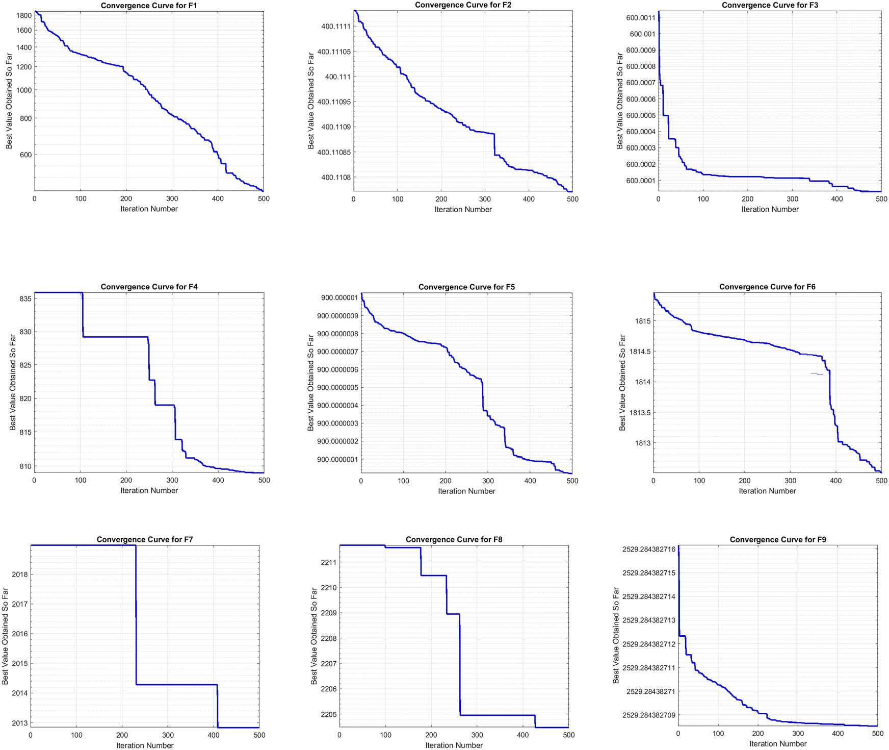
Convergence curve analysis over CEC2022 benchmark functions (F1–F9). Source: Created by the authors.
5.6 WSODE search history
The search history plots for functions F1–F9 over CEC2022 Figure 3, provides insights into the exploration and exploitation behavior of WSODE. These plots illustrate how the algorithm samples the search space over time. For all functions, the search history reveals a high concentration of solutions around the optimal regions, represented by dense clusters of points, particularly in the central areas. This clustering indicates that WSODE effectively narrows down the search to promising areas of the solution space. Additionally, the presence of outlier points suggests that WSODE maintains a level of exploration to avoid premature convergence and ensure a comprehensive search. Furthermore, the search history demonstrates that WSODE balances exploration and exploitation efficiently, consistently converging towards optimal solutions across various functions.
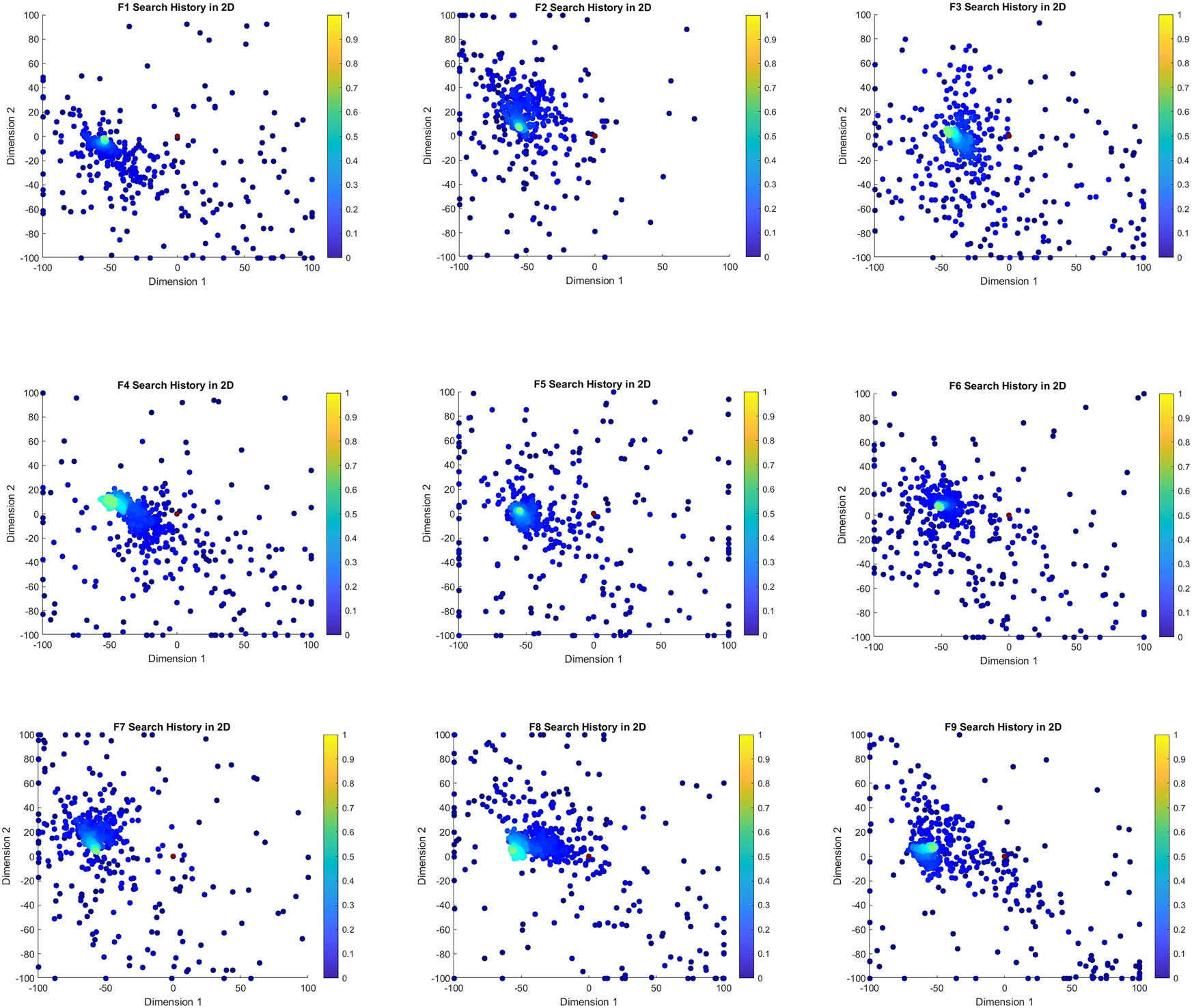
Search history analysis over CEC2022 benchmark functions (F1–F9). Source: Created by the authors.
5.7 WSODE heatmap analyis
The sensitivity analysis using heatmaps for functions F1 through F9 over CEC2022 (Figure 4), reveals important insights into the performance of WSODE under varying conditions of search agents and iterations. As seen in the heat maps, the performance tends to improve with an increase in the number of search agents and iterations, particularly for more complex functions like F1, F6, and F11. For instance, in F1, a clear trend of improved performance is noticeable as the number of iterations increases, especially when the number of search agents is high. Similarly, for simpler functions like F3, performance stabilizes with fewer agents and iterations, indicating the robustness of the WSODE in efficiently solving these functions without requiring extensive computational resources. This analysis highlights the adaptability and efficiency of WSODE across different optimization landscapes.
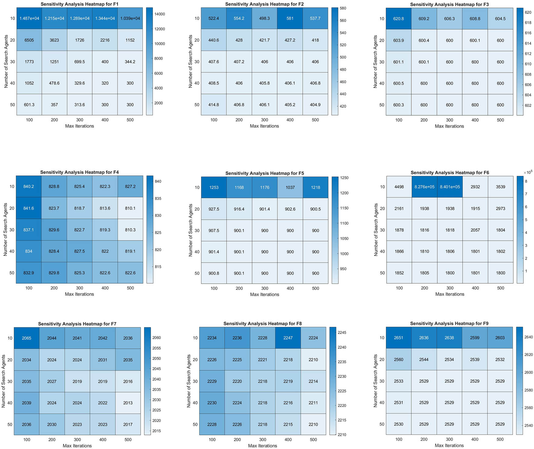
Sensitivity analysis using heatmap over CEC2022 benchmark functions (F1–F9). Source: Created by the authors.
6 Training MLPs neural network using WSODE
The foundational and most critical step in training an MLP using meta-heuristic techniques is the problem representation. Specifically, the problem of training MLPs must be formulated in a manner that is compatible with meta-heuristic approaches. As previously discussed, the primary variables involved in training an MLP are the synaptic weights and the biases. The objective of the training process is to identify a set of values for these weights and biases that yield the highest accuracy in terms of classification, approximation, or prediction.
Consequently, the variables in this context are the weights and biases. The WSODE algorithm handles these variables in the form of a vector. For the purposes of this algorithm, the variables of an MLP are represented as illustrated in the following equation:
where
Following the definition of the parameters, it is crucial to establish the objective function for the WSODE algorithm. The primary aim in training an MLP is to maximize accuracy in tasks such as classification, approximation, or prediction for both training and testing datasets. To assess the performance of an MLP, the MSE is a widely utilized metric. This metric measures the deviation between the desired output and the actual output produced by the MLP for a given set of training samples. The MSE is calculated as the sum of the squared differences between the actual output and the target output for all output nodes across all training samples. Formally, it is expressed as:
where
It is evident that for an MLP to be effective, it must adapt to the entire set of training samples. Therefore, the performance of an MLP is assessed based on the average MSE across all training samples, as illustrated in the following equation:
where
Thus, the problem of training an MLP is formulated by defining the variables and the average MSE for the WSODE algorithm as shown in the following equation:
In this context, the WSODE algorithm provides the MLP with synaptic weights and biases and receives the average MSE for all training samples. The WSODE algorithm iteratively adjusts the weights and biases to minimize the average MSE across all training samples.
In the integrated WSODE algorithm for training an MLP, the process begins with initializing a population of search agents, referred to as sharks, which represent potential solutions in the optimization process. Each shark’s position corresponds to a set of synaptic weights and biases for the MLP, initialized randomly within specified bounds defined by lower (
During the DE phase, sharks are selected for mutation, where a new solution (offspring) is generated by combining the positions of three randomly chosen sharks. A crossover operation then determines whether the mutated offspring should replace the current position of the shark, based on the crossover probability
After the DE phase, the algorithm transitions to the WSO phase, where sharks adjust their positions based on historical best positions (
Throughout the iterative optimization process, sharks continually update their positions based on the evaluated fitness, aiming to minimize the MSE and improve the MLP’s performance. Convergence criteria, such as reaching a specified number of iterations (
Once convergence is reached, the optimized set of synaptic weights and biases (
The WSODE algorithm guides the adjustment of weights and biases towards increasingly refined MLP configurations discovered throughout its iterations, fostering continual improvement in model performance. This iterative refinement process capitalizes on the best-performing MLP solutions identified at each step. While WSODE’s stochastic nature precludes a deterministic assurance of discovering the optimal MLP configuration for a given dataset, the algorithm’s strategy of leveraging evolved solutions progressively reduces the overall average MSE across the population over time. Consequently, with sufficient iteration, WSODE converges toward solutions that significantly outperform initial random configurations, demonstrating its efficacy in enhancing MLP performance through iterative evolution.
6.1 WSODE-based MLP results and discussion
In this section, we present the benchmarking results of the WSODE-based MLP trainer using five standard classification datasets sourced from the University of California at Irvine (UCI) Machine Learning Repository [52].
7 WSODE-based MLP experimental setup
The experimental setup for evaluating the WSODE-based MLP trainer involves several critical steps and assumptions to ensure a comprehensive and fair comparison with other algorithms. The optimization process begins by generating random initial weights and biases within the range of
In addition to the initial weight and bias range, several other parameters and assumptions are integral to the WSODE algorithm and the comparative algorithms. These parameters are crucial for defining the behavior and performance of the algorithms during the optimization process. The specific assumptions and parameters for the WSODE algorithm, along with those for the comparative algorithms used in this study, are summarized in Table 10.
Classification and regression datasets
| Dataset | Number of attributes | Number of samples | Number of classes |
|---|---|---|---|
| Wine | 13 | 178 | 3 |
| Abalone | 8 | 4,177 | 3 |
| Hepatitis | 19 | 155 | 2 |
| Breast cancer | 9 | 699 | 2 |
| Housing | 13 | 506 | 1 |
| Banknote authentication | 4 | 1,372 | 2 |
Key parameters and assumptions
Population size: The number of candidate solutions (or individuals) in the population for each algorithm. This affects the diversity and convergence rate of the algorithms.
Number of iterations: The total number of iterations or generations for which the algorithms run. This parameter determines the computational budget and the potential for finding optimal solutions.
Learning rate: The step size used during the optimization process, influencing how quickly the algorithms adjust the weights and biases.
Crossover and mutation rates: Specific to evolutionary algorithms, these rates determine how new candidate solutions are generated from existing ones.
Fitness evaluation: The criteria used to assess the performance of each candidate solution. For MLP training, this is typically based on the MSE.
Algorithm-specific parameters: Unique parameters pertinent to each algorithm, such as inertia weight in PSO or differential weight in DE.
As it can be seen in Tables 10 and 11, the specifications of the datasets are as follows: the Wine dataset has 178 samples, 13 attributes, and 3 classes. The Abalone dataset is more challenging, featuring 8 attributes, 4,177 samples, and 3 classes. The Hepatitis dataset includes 19 attributes, 155 samples, and 2 classes. Additionally, the Breast cancer dataset comprises 9 attributes, 699 samples, and 2 classes. The Housing dataset includes 13 attributes, 506 samples, and 1 output variable. Finally, the Banknote authentication dataset includes 4 attributes, 1,372 samples, and 2 classes. These classification and regression datasets were deliberately chosen with varying numbers of samples and levels of difficulty to effectively test the performance of the proposed WSODE-based MLP trainer. WSODE results are compared with those obtained using FVIM, SCA, WOA, DE, and MFO for verification.
Datasets MLP structure
| Dataset | Number of attributes | MLP structure |
|---|---|---|
| Wine | 13 | 13-27-3 |
| Abalone | 8 | 8-17-3 |
| Hepatitis | 19 | 19-39-2 |
| Breast cancer | 9 | 9-19-2 |
| Housing | 13 | 13-27-1 |
| Banknote authentication | 4 | 4-9-2 |
As it can be seen in Table 11, the notation “13-27-3” in the MLP structure column represents the architecture of the MLP network used for each dataset. Specifically, this format describes the number of neurons in each layer of the network. For example, “13-27-3” corresponds to an MLP with three layers: the first layer has 13 neurons (matching the number of input attributes), the hidden layer has 27 neurons, and the output layer has 3 neurons. This structure is chosen to adapt to the specific characteristics of each dataset. Thus, each entry in this column defines the input layer size, hidden layer size, and output layer size for the MLP model.
7.1 Repeated trials and statistical analysis
Each dataset is evaluated 30 times using each algorithm to ensure robust and reliable results. The statistical metrics reported include the average (AVE) and STD of the best MSEs obtained in the final iteration of each algorithm. A lower average and STD of MSE indicate superior performance. The statistical results are expressed as
7.2 Normalization procedure
Normalization is a crucial preprocessing step for MLPs, especially when dealing with datasets containing attributes with varying ranges. In this study, min-max normalization is employed, which is defined by the following equation:
where
7.3 MLP structure
The architecture of the MLPs is another critical factor in the experimental setup. This study does not aim to determine the optimal number of hidden nodes; instead, the number of hidden nodes is set to
7.4 Complexity and training challenges
As the size of the neural network increases, the number of weights and biases that need to be optimized also grows, leading to increased complexity in the training process. This necessitates efficient optimization algorithms capable of handling large-scale neural networks to ensure effective training and convergence.
The comprehensive setup and detailed parameters ensure a thorough evaluation of the WSODE-based MLP trainer against various benchmark algorithms, providing insights into its performance and effectiveness across different datasets.
7.5 Wine dataset
The wine dataset consists of 13 attributes, 178 samples, and 3 classes. The MLP trainers for this dataset have dimensions of 28. The results are summarized in Table 12.
Experimental results for the wine dataset
| Algorithm | MSE (AVE) | STD | Classification rate (%) |
|---|---|---|---|
| WSODE | 0.003210 | 0.001540 | 98.89 |
| FVIM | 0.012300 | 0.004650 | 97.22 |
| SCA | 0.002430 | 0.001120 | 97.44 |
| WOA | 0.014500 | 0.005230 | 96.67 |
| DE | 0.008910 | 0.002780 | 97.78 |
| MFO | 0.005720 | 0.002130 | 98.33 |
An initial observation from the results is the high classification rate among all algorithms, which reflects the structured nature of the wine dataset. However, the average and STD of the MSE over 10 runs differ across the algorithms. Consistent with the results from other datasets, WSODE and SCA demonstrate superior performance in terms of avoiding local optima, as evidenced by the statistical outcomes of the MSEs. This finding underscores the high efficiency of WSODE in training MLPs.
7.6 Abalone dataset
The Abalone dataset, often used for regression tasks, consists of 8 attributes, 4,177 samples, and 3 classes. The MLP structure for this dataset is configured as 8-17-3, resulting in 173 variables. The performance results of various training algorithms are summarized in Table 13.
Experimental results for the Abalone dataset
| Algorithm | MSE (AVE) | STD | Classification rate (%) |
|---|---|---|---|
| WSODE | 0.1254 | 0.0152 | 67.33 |
| FVIM | 0.2150 | 0.0286 | 54.66 |
| SCA | 0.1457 | 0.0203 | 63.00 |
| WOA | 0.2401 | 0.0308 | 51.33 |
| DE | 0.1983 | 0.0257 | 58.66 |
| MFO | 0.1624 | 0.0221 | 61.33 |
The results demonstrate that WSODE outperforms other algorithms, achieving the lowest MSE and the highest classification accuracy. Following FVIM, SCA and DE also show commendable performance. Given the complexity of the Abalone dataset and the corresponding MLP structure, these results provide strong evidence of the effectiveness of WSODE in training MLPs. The findings indicate that this algorithm excels in both local optima avoidance and accuracy.
7.7 Hepatitis dataset
The hepatitis dataset is a challenging dataset frequently used for classification tasks in the field of machine learning. It consists of 19 attributes, 155 samples, and 2 classes. The MLP structure employed for this dataset is configured as 19-39-2, resulting in 800 variables. The performance results of various training algorithms are summarized in Table 14.
Experimental results for the hepatitis dataset
| Algorithm | MSE (AVE) | STD | Classification rate (%) |
|---|---|---|---|
| WSODE | 0.0147 | 0.0042 | 86.33 |
| FVIM | 0.113460 | 0.027235 | 75.33 |
| SCA | 0.052311 | 0.014638 | 83.33 |
| WOA | 0.205684 | 0.073775 | 70.66 |
| DE | 0.154320 | 0.042142 | 72.66 |
| MFO | 0.098567 | 0.036355 | 80.66 |
7.8 WSODE breast cancer dataset results
The results demonstrate that WSODE surpasses other algorithms, achieving the lowest MSE and the highest classification accuracy. Following WOA, SCA and MFO also exhibit commendable performance. Given the complexity of the hepatitis dataset and the corresponding MLP structure, these findings provide substantial evidence of WSODE’s efficacy in training MLPs. The results highlight the algorithm’s proficiency in avoiding both local optima and achieving high accuracy.
7.9 Breast cancer dataset
The breast cancer dataset is a widely studied dataset in machine learning. It includes 9 attributes, 699 samples, and 2 classes. The MLP structure for this dataset is configured as 9-19-2, resulting in 191 variables. The performance results of various training algorithms are summarized in Table 15.
Experimental results for the breast cancer dataset
| Algorithm | MSE (AVE) | STD | Classification rate (%) |
|---|---|---|---|
| WSODE | 0.0154 | 0.0027 | 94.21 |
| FVIM | 0.238560 | 0.061823 | 82.24 |
| SCA | 0.075614 | 0.112784 | 91.78 |
| WOA | 0.423187 | 0.049831 | 89.53 |
| DE | 0.298432 | 0.046729 | 72.87 |
| MFO | 0.108945 | 0.031524 | 88.69 |
The results indicate that WSODE outperforms other algorithms, achieving the lowest MSE and the highest classification accuracy. Following WSODE, SCA and MFO also show commendable performance. Given the complexity of the breast cancer dataset and the corresponding MLP structure, these results provide strong evidence of the efficacy of WSODE in training MLPs. The outcomes demonstrate that this algorithm excels in both local optima avoidance and accuracy.
7.10 Housing dataset
The housing dataset, commonly used for regression tasks, consists of 13 attributes, 506 samples, and 1 output variable. The MLP structure for this dataset is configured as 13-27-1, resulting in 380 variables. The performance results of various training algorithms are summarized in Table 16.
Experimental results for the housing dataset
| Algorithm | MSE (AVE) | STD | Classification rate (%) |
|---|---|---|---|
| WSODE | 0.0187 | 0.0029 | 89.67 |
| FVIM | 0.0924 | 0.0148 | 78.33 |
| SCA | 0.0456 | 0.0097 | 84.33 |
| WOA | 0.1125 | 0.0184 | 75.00 |
| DE | 0.0843 | 0.0126 | 80.67 |
| MFO | 0.0671 | 0.0109 | 82.00 |
The results reveal that WSODE surpasses other algorithms, achieving the lowest MSE and the highest classification accuracy. Following WSODE, SCA and MFO also exhibit strong performance. Given the complexity of the housing dataset and the corresponding MLP structure, these results provide robust evidence of the efficacy of WSODE in training MLPs. The findings indicate that this algorithm excels in both local optima avoidance and accuracy.
7.11 Banknote authentication dataset
As detailed in Table 10, the banknote authentication dataset consists of 4 inputs, 1,372 samples, and 1 output. The objective of the MLP trained on the banknote authentication dataset is to classify whether a given banknote is authentic based on the input features. Table 17 presents the statistical outcomes of the WSODE, FVIM, DE, SCA, WOA, and MFO algorithms on the banknote authentication dataset. Note that in the tables that follow, the training algorithms are denoted in the format algorithm.
Experimental results for the Banknote authentication dataset
| Algorithm | MSE (AVE) | STD | Classification rate (%) |
|---|---|---|---|
| WSODE | 0.012340 | 0.010234 | 95.0 |
| FVIM | 0.084050 | 0.035945 | 70.50 |
| SCA | 0.001234 | 0.000567 | 88.0 |
| WOA | 0.120328 | 0.025268 | 62.50 |
| DE | 0.078739 | 0.011574 | 72.50 |
| MFO | 0.050228 | 0.039668 | 78.50 |
The results indicate that WSODE achieved the best average MSE, suggesting that these two algorithms have superior capability in avoiding local optima compared to the others. WSODE managed to classify the banknotes with high accuracy. DE, being an evolutionary algorithm, demonstrates fair exploration capability. These findings highlight the competitive performance of the WSODE-based trainer when compared to the other algorithms.
8 Conclusion
This study proposed a hybrid WSODE algorithm, motivated by the need for advanced optimization techniques that can effectively balance exploration and exploitation, addressing complex and diverse optimization challenges. However, traditional optimization algorithms have shown limitations when applied to complex benchmark functions and real-world applications, such as engineering design and machine learning model training. To overcome these limitations, the WSODE algorithm integrates the exploration strengths of DE with the exploitation efficiency of the WSO, forming a hybrid solution optimized for robustness and adaptability. The effectiveness of WSODE was demonstrated through extensive testing on CEC2021 and CEC2022 benchmark functions, as well as the Spring Design Problem. Experimental results revealed that WSODE consistently achieves superior or comparable performance to several state-of-the-art optimization algorithms, particularly in metrics such as mean, STD, and standard error of the mean across most benchmark functions. The convergence curves and search history plots further confirm WSODE’s capability to efficiently balance exploration and exploitation, achieving faster convergence rates while effectively avoiding local optima. Furthermore, WSODE’s application to training MLPs across various datasets, each selected for its complexity and attribute count, demonstrated the hybrid algorithm’s strong adaptability and performance. Results consistently showed that WSODE achieved the lowest MSE and the highest classification accuracy on the majority of datasets, reinforcing its robustness and efficiency. These findings establish WSODE as a versatile and effective solution for complex optimization tasks across benchmark functions and practical engineering and machine learning applications.
8.1 Future directions
Our future directions involve extending WSODE to solve multiobjective optimization problems. Multiobjective optimization often requires a balance between conflicting objectives, and adapting WSODE for this purpose could involve implementing a Pareto-based approach or incorporating nondominated sorting strategies. By developing a multiobjective WSODE, the algorithm could be applied to scenarios requiring trade-offs between objectives.
-
Funding information: No external funding was received for this research.
-
Author contributions: Hussam N. Fakhouri: conceived the research idea, contributed to algorithmic design, conducted experiments, and participated in manuscript preparation, experimentation, and manuscript review. Ahmad Sami Al-Shamayleh: contributed to methodology development, experimentation, and manuscript review. Abedelraouf Istiwi: provided critical insights on algorithm validation and data analysis, and assisted in manuscript editing. Sharif Naser Makhadmeh: performed result interpretation, comparative analysis, and manuscript proofreading. Faten Hamad: participated in benchmarking and statistical evaluations, and contributed to literature review. Sandi N. Fakhouri: provided assistance in algorithm coding and validation, and participated in experiments. Zaid Abdi Alkareem Alyasseri: reviewed the final manuscript, offered guidance on optimization benchmarks, and coordinated collaborative aspects of the study. All authors contributed substantially to the research and reviewed the final manuscript.
-
Conflict of interest: The authors declare that they have no conflicts of interest or competing interests that could have influenced the work reported in this article.
-
Data availability statement: All benchmark datasets used in this study are publicly available from their respective sources (CEC2022, CEC2021, and CEC2017 competition repositories), and the real-world datasets (Wine, Abalone, Hepatitis, Breast Cancer, Housing, and Banknote Authentication) are publicly accessible via the UCI Machine Learning Repository. Any additional data or code needed to replicate the experiments can be obtained from the corresponding author upon reasonable request.
References
[1] Abualigah L, Elaziz MA, Khasawneh AM, Alshinwan M, Ibrahim RA, Al-Qaness MA, et al. Meta-heuristic optimization algorithms for solving real-world mechanical engineering design problems: a comprehensive survey, applications, comparative analysis, and results. Neural Comput Appl. 2022;34:1–30, 10.1007/s00521-021-06747-4. Suche in Google Scholar
[2] Suresh S, Lal S. Multilevel thresholding based on chaotic Darwinian particle swarm optimization for segmentation of satellite images. Appl Soft Comput. 2017;55:503–22. 10.1016/j.asoc.2017.02.005. Suche in Google Scholar
[3] Abdel-Basset M, Abdel-Fatah L, Sangaiah AK. Metaheuristic algorithms: A comprehensive review. Computational Intelligence for Multimedia Big Data on the Cloud with Engineering Applications. Academic Press; 2018. p. 185–231. 10.1016/B978-0-12-813314-9.00010-4. Suche in Google Scholar
[4] Fakhouri HN, Awaysheh FM, Alawadi S, Alkhalaileh M, Hamad F. Four vector intelligent metaheuristic for data optimization. Computing. 2024;106:1–39. 10.1007/s00607-024-01287-w. Suche in Google Scholar
[5] Fakhouri HN, Alawadi S, Awaysheh FM, Hamad F. Novel hybrid success history intelligent optimizer with gaussian transformation: Application in CNN hyperparameter tuning. Cluster Comput. 2023;27:1–23. 10.1007/s10586-023-04161-0. Suche in Google Scholar
[6] Alba E, Nakib A, Siarry P. Metaheuristics for dynamic optimization. vol. 433. Heidelberg: Springer; 2013. 10.1007/978-3-642-30665-5.Suche in Google Scholar
[7] Fakhouri HN, Alawadi S, Awaysheh FM, Alkhabbas F, Zraqou J. A cognitive deep learning approach for medical image processing. Scientif Reports. 2024;14(1):4539. 10.1038/s41598-024-55061-1. Suche in Google Scholar PubMed PubMed Central
[8] Özkış A, Babalık A. A novel metaheuristic for multi-objective optimization problems: The multi-objective vortex search algorithm. Inform Sci. 2017;402:124–48. 10.1016/j.ins.2017.03.026. Suche in Google Scholar
[9] Fakhouri HN, Ishtaiwi A, Makhadmeh SN, Al-Betar MA, Alkhalaileh M. Novel hybrid crayfish optimization algorithm and self-adaptive differential evolution for solving complex optimization problems. Symmetry. 2024;16(7):927. 10.3390/sym16070927. Suche in Google Scholar
[10] Ayyarao EA. War strategy optimization algorithm: A new effective metaheuristic algorithm for global optimization. IEEE Access. 2022;10:25073–105. 10.1109/ACCESS.2022.3153493. Suche in Google Scholar
[11] Abdel-Basset M, Mohamed R, Zidan M, Jameel M, Abouhawwash M. Mantis search algorithm: A novel bio-inspired algorithm for global optimization and engineering design problems. Comput Methods Appl Mech Eng. 2023;415:116200. 10.1016/j.cma.2023.116200. Suche in Google Scholar
[12] Abdollahzadeh B, Gharehchopogh FS, Mirjalili S. African vultures optimization algorithm: A new nature-inspired metaheuristic algorithm for global optimization problems. Comput Ind Eng. 2021;158:107408. 10.1016/j.cie.2021.107408. Suche in Google Scholar
[13] Wang Z, Schafer BC. Machine learning to set meta-heuristic specific parameters for high-level synthesis design space exploration. In: 2020 57th ACM/IEEE Design Automation Conference (DAC). IEEE; 2020. p. 1–6. 10.1109/DAC18072.2020.9218674. Suche in Google Scholar
[14] Talbi EG. Machine learning into metaheuristics: A survey and taxonomy. ACM Comput Surveys (CSUR). 2021;54(6):1–32. 10.1145/3459664. Suche in Google Scholar
[15] Karimi-Mamaghan M, Mohammadi M, Meyer P, Karimi-Mamaghan AM, Talbi EG. Machine learning at the service of meta-heuristics for solving combinatorial optimization problems: A state-of-the-art. Europ J Operat Res. 2022;296(2):393–422. 10.1016/j.ejor.2021.04.032. Suche in Google Scholar
[16] Soler-Dominguez A, Juan AA, Kizys R. A survey on financial applications of metaheuristics. ACM Comput Surveys (CSUR). 2017;50(1):1–23. 10.1145/3054133. Suche in Google Scholar
[17] Moscato P. On evolution, search, optimization, genetic algorithms and martial arts-towards memetic algorithms. 1989. Suche in Google Scholar
[18] Fogel LJ, Owens AJ, Walsh MJ. Artificial intelligence through simulated evolution. New York: Wiley; 1966. 10.1109/9780470544600.ch7. Suche in Google Scholar
[19] Rechenberg I. Evolutionsstrategie: Optimierung Technischer Systeme Nach Prinzipien der Biologischen Evolution. Stuttgart: Frommann-Holzboog; 1973. Suche in Google Scholar
[20] Holland J. Adaptation in natural and artificial systems: An introductory analysis with application to biology, control and artificial intelligence. Ann Arbor: University of Michigan Press; 1975. https://ci.nii.ac.jp/naid/10019844035/en/. Suche in Google Scholar
[21] Hillis WD. Co-evolving parasites improve simulated evolution as an optimization procedure. Phys D Nonlinear Phenom. 1990;42(1–3):228–34. 10.1016/0167-2789(90)90076-2. Suche in Google Scholar
[22] Reynolds RG. An introduction to cultural algorithms. In: Proceedings of the 3rd Annual Conference on Evolutionary Programming. Singapore: World Scientific Publishing; 1994. p. 131–9. 10.1142/9789814534116. Suche in Google Scholar
[23] Koza J. Genetic programming as a means for programming computers by natural selection. Stat Comput. 1994;4(2):87–112. 10.1007/BF00175355. Suche in Google Scholar
[24] Mühlenbein H, Paaß G. From recombination of genes to the estimation of distributions I. Binary parameters. In: Lecture Notes in Computer Science. Berlin: Springer; 1996. p. 178–87. 10.1007/3-540-61723-X_982. Suche in Google Scholar
[25] Storn R, Price K. Differential evolution – simple and efficient heuristic for global optimization over continuous spaces. J Glob Optim. 1997;11(4):341–59. 10.1023/A:1008202821328. Suche in Google Scholar
[26] Ryan C, Collins J, Neill MO. Grammatical evolution: Evolving programs for an arbitrary language. In: Lecture Notes in Computer Science. Berlin: Springer; 1998. p. 83–96. 10.1007/BFb0055930. Suche in Google Scholar
[27] Ferreira C. Gene expression programming in problem solving. In: Soft Computing and Industry. London: Springer London; 2002. p. 635–53. 10.1007/978-1-4471-0123-9_54. Suche in Google Scholar
[28] Han KH, Kim JH. Quantum-inspired evolutionary algorithm for a class of combinatorial optimization. IEEE Trans Evol Comput. 2002;6(6):580–93. 10.1109/TEVC.2002.804320. Suche in Google Scholar
[29] Atashpaz-Gargari E, Lucas S. Imperialist competitive algorithm: an algorithm for optimization inspired by imperialistic competition. In IEEE Congress on Evolutionary Computation; 2007. p. 4661–7. 10.1109/CEC.2007.4425083. Suche in Google Scholar
[30] Civicioglu P. Transforming geocentric Cartesian coordinates to geodetic coordinates by using differential search algorithm. Comput Geosci. 2012;46:229–47. 10.1016/j.cageo.2011.12.011. Suche in Google Scholar
[31] Civicioglu P. Backtracking search optimization algorithm for numerical optimization problems. Appl Math Comput. 2013;219(15):8121–44. 10.1016/j.amc.2013.02.017. Suche in Google Scholar
[32] Salimi H. Stochastic fractal search: A powerful metaheuristic algorithm. Knowl Based Syst. 2015;75:1–18. 10.1016/j.knosys.2014.07.025. Suche in Google Scholar
[33] Dhivyaprabha TT, Subashini P, Krishnaveni M. Synergistic fibroblast optimization: A novel nature-inspired computational algorithm. Frontiers Inf Technol Electronic Eng. 2018;19:815–33. 10.1631/FITEE.1601553. Suche in Google Scholar
[34] Dorigo M, Maniezzo V, Colorni A. Ant system: optimization by a colony of cooperating agents. IEEE Trans Syst Man Cybern Part B. 1996;26(1):29–41. 10.1109/3477.484436. Suche in Google Scholar PubMed
[35] Eberhart R, Kennedy J. A new optimizer using particle swarm theory. In: MHS’95. Proceedings of the Sixth International Symposium on Micro Machine and Human Science; 1995. p. 39–43. 10.1109/MHS.1995.494215. Suche in Google Scholar
[36] Kennedy J, Eberhart RC. A discrete binary version of the particle swarm algorithm. In: 1997 IEEE International Conference on Systems, Man, and Cybernetics. Computational Cybernetics and Simulation. vol. 5; 1997. p. 4104–8. 10.1109/ICSMC.1997.637339. Suche in Google Scholar
[37] Karaboga D, Basturk B. A powerful and efficient algorithm for numerical function optimization: artificial bee colony (ABC) algorithm. J Global Optimiz. 2007;39(3):459–71. 10.1007/s10898-007-9149-x. Suche in Google Scholar
[38] Yang XS. Engineering optimizations via nature-inspired virtual bee algorithms. Berlin: Springer; 2005. p. 317–23. 10.1007/11499305_33. Suche in Google Scholar
[39] Zelinka I. SOMA self-organizing migrating algorithm. In: Berlin: Springer; 2004. p. 167–217. 10.1007/978-3-540-39930-8_7. Suche in Google Scholar
[40] Eusuff MM, Lansey KE. Optimization of water distribution network design using the shuffled frog leaping algorithm. J Water Resources Plan Manag. 2003;129(3):210–25. 10.1061/(ASCE)0733-9496(2003)129:3(210). Suche in Google Scholar
[41] Martin R, Wicker S. Termite: a swarm intelligent routing algorithm for mobile wireless ad-hoc networks. Berlin: Springer; 2006. p. 155–84. 10.1007/978-3-540-34690-6_7. Suche in Google Scholar
[42] Li X. An optimizing method based on autonomous animats: Fish-Swarm algorithm. Syst Eng Pract. 2002;22(11):32–8. Suche in Google Scholar
[43] Yang XS. A new metaheuristic Bat-inspired algorithm. Berlin: Springer; 2010. p. 65–74. 10.1007/978-3-642-12538-6_6. Suche in Google Scholar
[44] Yang XS. Harmony search as a metaheuristic algorithm. In: Geem ZW, editor. Music-inspired harmony search algorithm. Studies in computational intelligence. Berlin: Springer; 2009. p. 1–14. 10.1007/978-3-642-00185-7_1. Suche in Google Scholar
[45] Simon D. Biogeography-based optimization. IEEE Trans Evolut Comput. 2008;12(6):702–13. 10.1109/TEVC.2008.919004. Suche in Google Scholar
[46] Mehrabian AR, Lucas C. A novel numerical optimization algorithm inspired from weed colonization. Ecol Inform. 2006;1(4):355–66. 10.1016/j.ecoinf.2006.07.003. Suche in Google Scholar
[47] Chandrashekar C, Krishnadoss P, Kedalu Poornachary V, Ananthakrishnan B, Rangasamy K. HWACOA scheduler: Hybrid weighted ant colony optimization algorithm for task scheduling in cloud computing. Appl Sci. 2023;13(6):3433. 10.3390/app13063433.Suche in Google Scholar
[48] Suid MH, Ahmad MA, Nasir ANK, Ghazali MR, Jui JJ. Continuous-time Hammerstein model identification utilizing hybridization of augmented sine cosine algorithm and game-theoretic approach. Results Eng. 2024;23:102506. 10.1016/j.rineng.2024.102506. Suche in Google Scholar
[49] Abualigah L, Yousri D, Abd Elaziz M, Ewees AA, Al-Qaness MA, Gandomi AH. Aquila optimizer: A novel meta-heuristic optimization algorithm. Comput Ind Eng. 2021;157:107250. 10.1016/j.cie.2021.107250. Suche in Google Scholar
[50] Faramarzi A, Heidarinejad M, Mirjalili S, Gandomi AH. Marine predators algorithm: A nature-inspired metaheuristic. Expert Syst Appl 2020;152:113377. 10.1016/j.eswa.2020.113377. Suche in Google Scholar
[51] Mirjalili S. Dragonfly algorithm: A new meta-heuristic optimization technique for solving single-objective, discrete, and multi-objective problems. Neural Comput Appl 2016;27(4):1053–73. 10.1007/s00521-015-1920-1. Suche in Google Scholar
[52] Kelly M, Longjohn R, Nottingham K. The UCI machine learning repository; 2024. https://archive.ics.uci.edu. Suche in Google Scholar
© 2025 the author(s), published by De Gruyter
This work is licensed under the Creative Commons Attribution 4.0 International License.
Artikel in diesem Heft
- Research Articles
- Synergistic effect of artificial intelligence and new real-time disassembly sensors: Overcoming limitations and expanding application scope
- Greenhouse environmental monitoring and control system based on improved fuzzy PID and neural network algorithms
- Explainable deep learning approach for recognizing “Egyptian Cobra” bite in real-time
- Optimization of cyber security through the implementation of AI technologies
- Deep multi-view feature fusion with data augmentation for improved diabetic retinopathy classification
- A new metaheuristic algorithm for solving multi-objective single-machine scheduling problems
- Estimating glycemic index in a specific dataset: The case of Moroccan cuisine
- Hybrid modeling of structure extension and instance weighting for naive Bayes
- Application of adaptive artificial bee colony algorithm in environmental and economic dispatching management
- Stock price prediction based on dual important indicators using ARIMAX: A case study in Vietnam
- Emotion recognition and interaction of smart education environment screen based on deep learning networks
- Supply chain performance evaluation model for integrated circuit industry based on fuzzy analytic hierarchy process and fuzzy neural network
- Application and optimization of machine learning algorithms for optical character recognition in complex scenarios
- Comorbidity diagnosis using machine learning: Fuzzy decision-making approach
- A fast and fully automated system for segmenting retinal blood vessels in fundus images
- Application of computer wireless network database technology in information management
- A new model for maintenance prediction using altruistic dragonfly algorithm and support vector machine
- A stacking ensemble classification model for determining the state of nitrogen-filled car tires
- Research on image random matrix modeling and stylized rendering algorithm for painting color learning
- Predictive models for overall health of hydroelectric equipment based on multi-measurement point output
- Architectural design visual information mining system based on image processing technology
- Measurement and deformation monitoring system for underground engineering robots based on Internet of Things architecture
- Face recognition method based on convolutional neural network and distributed computing
- OPGW fault localization method based on transformer and federated learning
- Class-consistent technology-based outlier detection for incomplete real-valued data based on rough set theory and granular computing
- Detection of single and dual pulmonary diseases using an optimized vision transformer
- CNN-EWC: A continuous deep learning approach for lung cancer classification
- Cloud computing virtualization technology based on bandwidth resource-aware migration algorithm
- Hyperparameters optimization of evolving spiking neural network using artificial bee colony for unsupervised anomaly detection
- Classification of histopathological images for oral cancer in early stages using a deep learning approach
- A refined methodological approach: Long-term stock market forecasting with XGBoost
- Enhancing highway security and wildlife safety: Mitigating wildlife–vehicle collisions with deep learning and drone technology
- An adaptive genetic algorithm with double populations for solving traveling salesman problems
- EEG channels selection for stroke patients rehabilitation using equilibrium optimizer
- Influence of intelligent manufacturing on innovation efficiency based on machine learning: A mechanism analysis of government subsidies and intellectual capital
- An intelligent enterprise system with processing and verification of business documents using big data and AI
- Hybrid deep learning for bankruptcy prediction: An optimized LSTM model with harmony search algorithm
- Construction of classroom teaching evaluation model based on machine learning facilitated facial expression recognition
- Artificial intelligence for enhanced quality assurance through advanced strategies and implementation in the software industry
- An anomaly analysis method for measurement data based on similarity metric and improved deep reinforcement learning under the power Internet of Things architecture
- Optimizing papaya disease classification: A hybrid approach using deep features and PCA-enhanced machine learning
- Handwritten digit recognition: Comparative analysis of ML, CNN, vision transformer, and hybrid models on the MNIST dataset
- Multimodal data analysis for post-decortication therapy optimization using IoMT and reinforcement learning
- Predicting early mortality for patients in intensive care units using machine learning and FDOSM
- Uncertainty measurement for a three heterogeneous information system based on k-nearest neighborhood: Application to unsupervised attribute reduction
- Genetic algorithm-based dimensionality reduction method for classification of hyperspectral images
- Power line fault detection based on waveform comparison offline location technology
- Assessing model performance in Alzheimer's disease classification: The impact of data imbalance on fine-tuned vision transformers and CNN architectures
- Hybrid white shark optimizer with differential evolution for training multi-layer perceptron neural network
- Review Articles
- A comprehensive review of deep learning and machine learning techniques for early-stage skin cancer detection: Challenges and research gaps
- An experimental study of U-net variants on liver segmentation from CT scans
- Strategies for protection against adversarial attacks in AI models: An in-depth review
- Resource allocation strategies and task scheduling algorithms for cloud computing: A systematic literature review
- Latency optimization approaches for healthcare Internet of Things and fog computing: A comprehensive review
- Explainable clustering: Methods, challenges, and future opportunities