Construction of classroom teaching evaluation model based on machine learning facilitated facial expression recognition

Dongdong Ge; Zhendong Zhang

doi:10.1515/jisys-2024-0453

Article Open Access

Construction of classroom teaching evaluation model based on machine learning facilitated facial expression recognition

Dongdong Ge and Zhendong Zhang

Published/Copyright: September 16, 2025

Published by

Become an author with De Gruyter Brill

Submit Manuscript Author Information

From the journal Journal of Intelligent Systems Volume 34 Issue 1

Abstract

This study proposes a machine learning (ML) framework to overcome emotion recognition challenges in classroom environments, where high facial expression similarity and complex postural backgrounds hinder the accurate analysis. First, the histogram of oriented gradients (HOGs) was used to extract seven facial expression features. Second, comparative analysis of six ML algorithms identified support vector machine (SVM) as the optimal classifier. Third, grid search with cross-validation enhanced SVM’s recognition performance by 13.9% accuracy, 11.3% precision, and 13.8% recall improvement. Fourth, students’ facial expressions were recognized using HOG and the optimized SVM during eight course tasks. A classroom teaching effect evaluation model was constructed to predict students’ learning concentration scores according to the positive degree of different facial expressions. Absolute error, relative error, scatter, and violin plots all demonstrate that the predicted concentration score is strongly linearly correlated with actual mission score and final grade; mean absolute errors were 1.95 and 3.3, while mean relative errors were 2.57 and 4.42%, respectively. This study provides a reliable new method for intervening in students’ learning concentration in advance and fostering the quality of classroom teaching.

Keywords: facial expression recognition; machine learning; support vector machine; optimization; teaching evaluation model

Nomenclature

ERM: Empirical risk minimization
HOG: Histogram of oriented gradients
ML: Machine learning
NN: Neural network
SRM: Structural risk minimization
SVM: Support vector machine

1 Introduction

Currently, machine learning (ML) is the closest intelligent learning method to the human brain [1]. With the development of big data and artificial intelligence technology, today, ML algorithms have become more intelligent and more efficient at processing various types of inventory data [2,3]. This has enabled more and more breakthroughs in the fields of economy [4], engineering [5,6], medicine [7], and education [8,9].

Benbouras enhanced the effectiveness of artificial neural network (NN) methods by using nine hybrid metaheuristic algorithms, which were applied for landslide mapping [10]. Wang et al. proposed a weighted ensemble strategy hybrid method that combines intelligent optimization algorithms and ensemble learning and can identify gang-related arson cases; they used the differential evolution algorithm to optimize the parameters and combination weights of the classifier [11]. Westerveld et al. proposed an ML method to predict transitions in the status of food security using transferable features [12]. Gupta et al. classified the evolutionary pathogenic proteins of bacteria by constructing a pathogenic protein database and an optimized support vector machine (SVM) algorithm; the constructed SVM classifier achieved an accuracy of 81.72% on the test dataset [13]. Zidi et al. built a theft detection dataset and developed an ML-based solution for automated theft identification [14]. ML approaches were also used to extract hidden theft detection information from smart meter data, and the model performance could be improved by 10%. Wu and Sun proposed an ensemble learning method based on self-adaption quantum genetic algorithm for the detection of civil aviation fatigue; in a related experiment, a detection accuracy of 98.5% was achieved [15]. Rashid et al. proposed a vision-based Bayesian filtering algorithm, which tracked the object as a whole rather than a point-based method [16]. Carnevali et al. proposed a graph-based method for positive and unlabeled learning, using a few positive documents and unlabeled documents to retrieve a set of “interest” documents from a textual collection [17].

In the field of education, how to effectively capture students’ learning status and emotional feedback has always been a focus of teachers’ attention. Traditional teaching methods often rely on teachers’ intuitive judgments and post-class feedback. Consequently, this often has problems such as strong subjectivity and poor timeliness. Moreover, AI is gradually penetrating into all aspects of education, bringing new opportunities for supporting smarter education. In the era of AI, ML approaches for smarter education are gaining traction. Accordingly, by ML facial expression recognition, it could be possible to better address them in the related education environment and to better prepare construction of classroom teaching evaluation model for smarter education.

However, the collected facial expression images are affected by many factors in the classroom such as lighting, occlusion, distance, and the resolution of the acquisition device, all of which greatly reduce the accuracy of algorithmic recognition. Therefore, facial expression recognition in real classroom scenarios remains a challenging task.

Accordingly, the contributions of this article are summarized as follows:

The histogram of oriented gradient (HOG) method is used to calculate the gradient direction histogram of facial images, which is used to extract compact and discriminative high-quality expression feature vectors.
The SVM with the highest accuracy for facial expression recognition is selected through the comparison of six ML algorithm tests.
Thirty-six hyperparameter combinations of SVM are optimized by grid search and cross-validation, thereby effectively improving the accuracy of facial expression recognition.
A classroom teaching effect evaluation model based on ML facial expression recognition is constructed. Both the effectiveness and predictive performance of the proposed model are systematically evaluated through the model-predicted concentration score, actual mission score, final grade, absolute errors, relative errors, scatter plots, and violin plots.

This article is structured as follows: The literature review is presented in Section 2, while Section 3 presents the comparison tests of six ML algorithms for facial expression recognition. Section 4 describes the optimization process of the SVM algorithm, and Section 5 describes the construction process of the classroom teaching evaluation model. Experimental verification and related discussion are also reported in Section 5. The conclusion is presented in Section 6.

2 Related works

Considerable efforts have been made to develop ML that can effectively support smarter education. Lu [18] and Huang [19] used ML methods to predict the performance of students, which enables early intervention in at-risk students to improve their chances of obtaining course credits. Nahar et al. explored the logical relationship between semester grades and classroom participation using manually collected data on classroom participation, semester grades, and accompanying tests [20]. Jong et al. proposed that an online programming system could save considerable manpower and costs when collecting information and data about course activities; their system recorded useful student operation data, which they used to predict whether students will encounter learning difficulties [21]. Cardona et al. found that NN and SVM algorithms are the most commonly used algorithms for data mining in the educational context [22,23]. Hooshyar et al. highlighted the importance of identifying all at-risk students to correctly distinguish between negative and positive samples when predicting students’ learning effect [24]. To optimize pedagogical preparation, Rashid et al. proposed an ML model, which used students’ past attendance records for training to find a pattern of classroom attendance and predict the accurate class intensity on any future date [25].

Facial expressions are one of the most important ways for humans to express their own emotions and convey emotions to others. Mehrabian proposed the famous formula of emotional expression [26], which states that about 55% of information is transmitted through facial expressions, much higher than information transmitted through vocalization (38%) and language (7%). Facial expression recognition data can be used to analyze students’ learning status and teachers’ teaching status; it also provides a new dimension to evaluate classroom effectiveness [27,28]. Zheng et al. made full use of both class label information and local spatial distribution information of samples and proposed a new algorithm for facial expression recognition with discriminant ability [29]. Zhi et al. established an optimization model based on three-dimensional convolutional NN; combined with statistical probability correlation and adaptive subsequence matching algorithms, their model achieved the prediction of facial expressions [30]. Tseng and Chen recognized the expression changes of students by measuring the distance changes of key facial features such as eyebrows, eyes, and mouth [31].

In addition, Zhang et al. encoded the skeleton-based action instance as a tensor and proposed a method to evaluate students’ class state by adding action recognition [32]. Cai [33] and Yang [34] proposed comprehensive methods to predict students’ mood in class by combining the characteristics of video action recognition and general student behavioral recognition. Holifield et al. proposed the concept of classroom concentration, namely, active classroom actions including reading aloud, listening to the teacher, and asking or answering questions [35]. Gaddam et al. proposed a network using ResNet50 to classify human facial emotions using static images, which produced better results than the existing models [36]. Lu et al. proposed a face recognition algorithm based on stacked autoencoder and local binary pattern. The results showed that the recognition rate of the algorithm on Yale database reached 99.05% [37]. To monitor and analyze learners’ behaviors in real time, Zhao and Qiu proposed a dual-stream-coded image sentiment analysis method based on background actions and facial expressions [38].

In summary, facial expression recognition research is a cross-disciplinary subject that involves computer vision, psychology, statistics, and other disciplines. At present, the accuracy of facial expression recognition in the classroom cannot fully meet the requirements for the construction of an intelligent classroom teaching evaluation model. In addition, how to clarify the logical relationship between variables such as students’ learning concentration score, actual mission score, and final grade, how to accurately construct a classroom teaching effect evaluation model based on ML facial expression recognition, and how to comprehensively evaluate such models all need further in-depth exploration.

3 Comparison of ML algorithm tests

3.1 Methodology

HOG is a feature extraction method for object detection and image classification processes. This method divides the image into several small cells and calculates a histogram of gradient directions in each cell. These histograms are concatenated into a vector, which forms the feature description of the image. The implementation steps of HOG are as follows:

S1: Image preprocessing.
S2: Gradient computation. The gradient magnitude and direction for each pixel in the image are calculated using operators such as Sobel. The gradients at the pixel point (x, y) are represented as follows:

(1) G x ( x , y ) = H ( x + 1 , y ) − H ( x − 1 , y ) ,

(2) G y ( x , y ) = H ( x , y + 1 ) − H ( x , y − 1 ) ,

where G _x(x, y), G _y(x, y), and H(x, y) represent the horizontal gradient, vertical gradient, and pixel value, respectively. The magnitude and the direction of gradients are denoted by equations (3) and (4):

(3) G ( x , y ) = G x ( x , y ) 2 + G y ( x , y ) 2 ,

(4) α ( x , y ) = tan − 1 G y ( x , y ) G x ( x , y ) .

S3: Cell division.
S4: Accumulation HOG.
S5: Normalization. The histogram is normalized within each cell using L2-norm (equation (5)).

(5) v = v ∣ v ∣ 2 + ε 2 ,

where v denotes the histogram within a block, and ɛ represents a small constant to prevent division by zero.

S6: Generation feature vector.

As a typical ML method, the main advantage of SVM is that it adopts the structural risk minimization (SRM) principle. The conventional NN uses the traditional empirical risk minimization (ERM) principle. ERM only seeks the minimum value of the training error, while SRM seeks the minimum value of the upper limit of the generalization error, which is composed of the sum of training error and confidence. Compared with ERM, SRM has been proved to be more effective in solving general classification and regression problems. The implementation process of SVM mainly includes the following four steps:

S1: Selecting the kernel function.
S2: Constructing the objective function. This objective function usually includes the minimization of model complexity and the maximization of classification margin and can be represented as a convex optimization problem.
S3: Solving the optimization problem. The objective function is solved through optimization algorithms (such as sequential minimal optimization or gradient descent) to obtain the optimal hyperplane parameters.
S4: Training the model. Training set samples and hyperplane parameters are used to train the model, resulting in a classifier that can accurately classify new samples.

Here are the details:

Suppose that all input parameters form a set of vectors x _i, and y _i is the sample label. When the number of samples is N, the sample set is defined as {(X _i, Y _i)}. Then, the relationship between the output and input of the SVM can be approximately expressed by equation (6):

(6) Y = f ( X ) = W ⋅ ϕ ( X ) + b ,

where ϕ(x) represents the nonlinear mapping coefficient from the input space X to the high-dimensional feature space. W and b are hyperplane parameters, which are estimated by minimizing regularized risk functions (equations (7) and (8)):

(7) Minimize : 1 2 ∥ W ∥ 2 + C 1 N ∑ i = 1 N L ε ( Y i , f ( X i ) ) ,

(8) L ε ( Y i , f ( X i ) = 0 ∣ Y i − f ( X i ) ∣ ≤ ε ∣ Y i − f ( X i ) ∣ − ε others ,

where ∥W∥² is a regularization term, which can be called “structured risk.” Minimizing ∥W∥² can flatten the function maximally. The second term in equation (7) is the empirical error, which is measured by the loss function; this second term is called “empirical risk,” where ɛ is the radius of the tube defined and C is a penalty parameter used to determine the trade-off between training error and model flatness. By introducing the positive relaxation variables ζ _i and ζ _i ^*, the objective function and boundary conditions are transformed into equation (9):

(9) Minimize: 1 2 ∥ W ∥ 2 + C 1 N ∑ i = 1 N L ε ( Y i , f ( X i ) ) Subject to: Y i − W ⋅ ϕ ( x i ) − b ≤ ε + ζ i W ⋅ ϕ ( x i ) + b − Y i ≤ ε + ζ i ⁎ , i = 1 , … , N ζ i ≥ 0 ζ i ⁎ ≥ 0 .

By introducing the kernel functions K(X _i, X _j), equation (6) is transformed into equation (10):

(10) Y = f ( X ) = ∑ i = 1 N ( α i − α i ⁎ ) K ( X i , X j ) + b ,

where i and j represent different samples and α_i and α_i* are Lagrange multipliers. Therefore, the objective function equation (9) is transformed into equation (11), and W and b are solved.

(11) Minimize: 1 2 ∑ i = 1 N ∑ j = 1 N ( α i − α i ⁎ ) ( α j − α j ⁎ ) ⋅ K ( X i , X j ) − ε ∑ i = 1 N ( α i − α i ⁎ ) + ∑ i = 1 N Y i ( α i − α i ⁎ ) Subject to: ∑ i = 1 N ( α i − α i ⁎ ) = 0 α i , α i ⁎ ∈ [ 0 , C ] .

3.2 Comparison of ML algorithm tests

The implementation process of ML facilitated facial expression recognition (Figure 1) mainly includes six steps:

S1: Data acquisition, i.e., collecting the required facial expression images.
S2: Data preprocessing. To improve the training efficiency and accuracy of the model, the images are subjected to size standardization, normalization, and data augmentation. The data are then divided into training set and testing set.
S3: Feature extraction. By dimensionality reduction, feature fusion, and feature encoding of facial images, compact and discriminative feature vectors are obtained.
S4: Model selection and training. ML models are selected and trained using data features and data labels.
S5: Model evaluation. The performance of the trained model is evaluated by the test set. Evaluation indicators include accuracy, precision, and recall.
S6: Model optimization. To improve the generalization ability, the models are optimized according to the evaluation results, including hyperparameter optimization, model fusion, and feature selection.

Figure 1

Process of ML facilitated facial expression recognition. Source: Created by the authors.

To select an accurate and efficient method for the recognition of facial expressions, in the experiment presented in this section, images from the Jaffe database [39,40] were used as experimental subjects. Seven facial expression features (i.e., angry, disgust, fear, happy, neutral, sad, and surprise) were extracted using the HOG method, as shown in Figure 2. A total of 80% of the data were randomly selected for model training, and the remaining 20% were used for testing. Six ML algorithms (i.e., K-nearest neighbors (KNN), decision tree, naive Bayes, logistic regression, random forest, and SVM) were used for recognition training. As software environment, Python version 3.12 was used. The test results were evaluated using the three indicators of accuracy (equation (12)), precision (equation (13)), and recall (equation (14)). Herein, TP (true positive) and FP (false positive) denote the numbers of correct and incorrect predictions for the classification, respectively; TN (true negative) and FN (false negative) represent the numbers of correct and incorrect predictions for the classification. The results are shown in Table 1 and Figure 3.

(12) Accuracy = TP + TN TP + TN + FP + FN ,

(13) Precision = TP TP + FP ,

(14) Recall = TP TP + FN .

Figure 2

Facial expression samples. Source: Derived from the Jaffe database [39,40].

Table 1

Comparison of recognition results of six algorithms (%)

S/N	Indicator	KNN	SVM	Decision tree	Naive Bayes	Logistic regression	Random forest
1	Accuracy	67.4	83.7	51.2	67.4	48.8	81.4
2	Precision	72.4	86.4	50.9	68.4	54.4	82.3
3	Recall	65.5	82.9	52.9	67.3	50.5	81.4

Figure 3

Comparison of recognition results of six algorithms. Source: Created by the authors.

The results of the analysis are presented as follows:

The fluctuation range of the three indicator values of each algorithm remains within 5%, indicating that the three indicators maintain a high degree of consistency.
Most algorithms have high precision values, while the accuracy results are relatively conservative.
The results show that SVM achieves the best recognition results, followed by random forest, with both algorithms achieving accuracy levels exceeding 80%. The recognition results of decision tree and logistic regression are relatively poor, with accuracy levels of only 51.2 and 48.8%, respectively.

Based on the analysis presented earlier, SVM with the highest accuracy rate was selected for students' facial expression recognition in the classroom.

4 Hyperparameter optimization

ML provides data support for the design and optimization of smart education. However, as ML algorithms are often directly used in the application of facial expression recognition, algorithms that do not conduct hyperparameter optimization can seriously undermine the fitting and accuracy of the model. In addition, the impact of different independent variable datasets on the classification performance of the model also needs to be clarified.

Currently, the main methods for hyperparameter optimization include random search, greedy search, and grid search. Random search identifies the optimal hyperparameter by randomly sampling various combinations of hyperparameters. However, random search does not cover all possible hyperparameter combinations, nor can it adjust its next step based on the tuning results of the previous step. These limitations imply that the method cannot guarantee that a good combination of hyperparameters can be found. Greedy search attempts to improve model performance by setting the values of hyperparameters one by one. Greedy search adopts the concept of stepwise optimization and local optimization, i.e., each time a hyperparameter is selected for optimization, other hyperparameters remain fixed (or have already been optimized), until all hyperparameters are optimized. Thus, the disadvantage is that it may identify a local optimum instead of the global optimum.

Grid search seeks the optimal hyperparameter by iterating through all possible combinations of hyperparameters. First, each hyperparameter is linked to a set of candidate values. These values are generated as Cartesian products, forming a grid of hyperparameter combinations. Then, grid search is used to train the model for each combination of hyperparameters. Moreover, cross-validation is used to accurately evaluate the effect of each combination of hyperparameters, thereby finding the best performance combination.

To improve the accuracy of SVM for facial expression recognition, grid search and K-fold cross-validation were used to optimize hyperparameters (namely, penalty coefficient C and kernel function coefficient γ) of SVM. The candidate values of hyperparameters are shown in Table 2, and a total of 36 different combinations of hyperparameters had to be evaluated. The specific steps of K-fold cross-validation are as follows:

S1: The original training set is evenly divided into K subsets (folds), such as taking K as 5.
S2: Each subset is set as the validation set in turn, and the remaining K − 1 subsets are used as the training set for K rounds of training and validation. After each verification, the performance metrics of the model are calculated.
S3: The average of the performance metrics of K times of validation is taken as the performance estimate of the model on the entire dataset.

Table 2

The Candidate values of the hyperparameters

S/N	Hyperparameter	Candidate value	Candidate value	Candidate value	Candidate value	Candidate value	Candidate value
1	C	0.0001	0.01	0.1	1	2	10
2	Y	0.001	0.1	0.1	1	10	100

After conducting fivefold cross-validation on 36 sets of hyperparameter combinations, the optimal hyperparameter combination (C = 2, γ = 10) with the best performance was obtained. Herein, the three performance indicators (accuracy, precision, and recall) of SVM were 95.3, 96.2, and 94.3%, respectively. Compared with the initial state, the three indicators increased by 13.9, 11.3, and 13.8%, respectively. This increase demonstrates that the cross-validation makes full use of all samples in the dataset, ensuring that each sample participates in both training and validation, thereby cross-validation effectively prevents both overfitting and underfitting and ensures that the evaluation results are highly reliable. In addition, by conducting multiple evaluations on different training and validation sets, the generalization ability of the model can be better evaluated and the hyperparameter combination that performs best on the validation set is obtained.

5 Verification result

5.1 Constructing the teaching effect evaluation model

This section describes an experiment, where the course of “artificial intelligence” is taken as the experimental object and facial expression images were collected from a total of 40 students during class. Facial expressions are recognized using the HOG and optimized SVM model. Scores are allocated based on the positive learning response of students’ different expressions, and a classroom teaching evaluation model to predict students’ learning concentration score is constructed. Finally, the predicted mean concentration score (i.e., the mean score of eight course missions), actual mission score (i.e., the actual score given by the teacher based on the quality of the mission completed by a student), and final grade (i.e., the final grade based on student’s attendance, class performance, and mission completion) are analyzed. The construction process of the classroom teaching evaluation model is depicted in Figure 4, and the main steps are explained as follows:

S1: Data acquisition. Facial expression images of each student were captured at the 2nd, 5th, 10th, 15th, 20th, 24th, 28th, 32nd, 35th, and 38th min of each class (10 times in total) through a camera located in front of the students.
S2: Data preprocessing. The images were subjected to size normalization, grayscale, and enhancement processing to reduce both noise and interference and improve the reliability of dataset recognition.
S3: Feature extraction. Compact and discriminative feature vectors were extracted from the captured images using the HOG method. Facial expressions encountered in the classroom include excited, thinking, neutral, daze, and tired.
S4: Model training. The optimized SVM model was trained using the training dataset.
S5: Assignment of scores to the output results. After SVM has output the facial expression recognition results, it assigned scores based on Table 3. The student’s concentration scores for this class were calculated using equation (15), where S _i represents the concentration score for the ith class. P _excited, P _thinking, P _neutral, P _daze, and P _tired represent the probability values for the model outputting excited, thinking, neutral, daze, and tired expressions for the students in this class.

(15) S i = 100 × P excited + 80 × P thinking + 70 × P neutral + 40 × P daze + 30 × P tired .

S6: Predicting the students’ concentration scores in the course. The predicted mean concentration scores Q _k during all missions were calculated using equation (16), where N represents the number of class sessions for the eight missions in the course.
(16) Q k = 1 N ∑ i = 1 N S i .
S7: Evaluation of the prediction results. The predicted mean concentration score Q _k, actual mission score R _k, and final grade Z _k were comprehensively analyzed. The accuracy and reliability of the prediction results were evaluated.
S8: Reflection and improvement. Based on the predicted results, classroom activities for students with lower predicted concentration scores can be amended in advance to enhance the learning effectiveness of at-risk students and improve their academic performance.

Figure 4

Construction process of the classroom teaching evaluation model. Source: Created by the authors.

Table 3

Expression score table

Expression	Excited	Thinking	Neutral	Daze	Tired
Score	100	80	70	40	30

5.2 Analysis

In this subsection, the predictive performance of the proposed model is evaluated by analyzing the predicted single mission concentration score E _k, the predicted mean concentration score Q _k, the actual mission score R _k, and the final grade Z _k for each student.

Figure 5 presents the results of the predicted single mission concentration score and predicted mean concentration score, where M1–M8 are the mission numbers and Q is the predicted mean concentration score. The analysis is presented as follows:

The predicted concentration scores vary among different missions, indicating that students’ actual performance varies across different missions. Student ID30 had the largest variation between predicted scores (19). Moreover, this student was the only one whose scores were all below 60. The student showed the highest frequency of daze and tired expressions. The student’s actual learning enthusiasm was also the lowest of all students in the actual classroom.
The predicted scores of 30 students (75% of the total) were within 10 points of each other. The average floating value of all students’ predicted scores was 8.2 points. This result indicates that the predictive performance of the developed model is relatively stable, and its generalization performance is good during all teaching periods of the course.

Figure 5

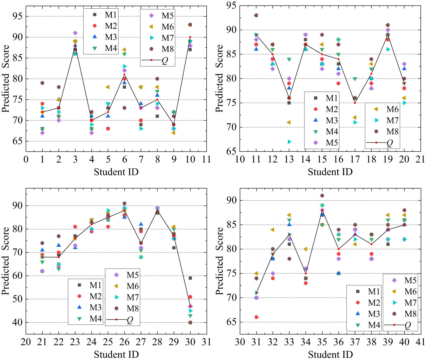
The predicted single mission concentration score and mean concentration score. Source: Created by the authors.

To analyze the correlation and fitting relationship among predicted mean concentration score, actual mission score, and final grade, a scatter plot of these three variables is drawn, as shown in Figure 6. The analysis is presented as follows:

The Pearson coefficient between final grade and predicted mean concentration score is 0.97, indicating a strong linear correlation between them. The fitting curve of these two variables is shown in equation (17), with a determination coefficient of R ² = 0.94. When fitting with a quadratic equation, the curve is given by equation (18), which achieves a better fitting effect with a determination coefficient of 0.96.
(17) z = 0.84 x + 15.93

(18) z = − 0.008 x 2 + 2 x − 26.3
A strong linear correlation was also found between actual mission score and predicted score, with a Pearson coefficient of 0.98. The fitting curves of the linear equation and the quadratic equation are shown in equations (19) and (20), respectively, with a determination coefficient of 0.96, indicating similar fitting effects.

(19) y = 1.18 x − 13.71

(20) y = 0.0015 x 2 + 0.96 x − 5.98

Figure 6

Scatter plot. Source: Created by the authors.

Figure 7 demonstrates the predicted mean concentration score, actual mission score, and final grade of all students. Figure 8 shows the absolute error between the predicted mean concentration score, the actual mission score, and the final grade. Figure 9 presents violin plots, which mainly evaluate the model from the dimensions of error probability density distribution, error median, error Kernel density distribution, and quartile range. The results of the analysis are presented as follows:

The change trends of the three curves (Figure 7) are basically consistent. The predicted mean concentration scores of four students remain below 70, including ID9 (69), ID21 (68), ID22 (68), and ID30 (47). The actual mission scores of these students are 66, 64, 70, and 42, with final grades of 74, 73, 76, and 50, respectively. This result indicates that by predicting mean concentration scores, actual mission scores and even the interval of final grades can be predicted well. Consequently, based on the predicted scores, it is possible to intervene in the classroom activities of students with low concentration scores in advance, thereby improving the academic performance of at-risk students.
Compared with the final grade, the absolute error between predicted mean concentration score and actual mission score is smaller. The final grade considers factors such as student attendance and additional points; therefore, the final grade is slightly higher than the predicted mean concentration score. The mean absolute errors between predicted mean concentration scores as well as actual mission scores and final grades were 1.95 and 3.3, respectively.
The probability density distribution of the error between predicted mean concentration scores as well as actual mission scores and final grades follows a basic normal distribution. The maximum error between predicted mean concentration scores and actual mission scores is 5 points. Similarly, the maximum error between predicted mean concentration scores and final grades is 8 points.
The distribution of errors between predicted mean concentration scores and actual mission scores is more concentrated, with a smaller quartile range.

Figure 7

The curves of three scores. Source: Created by the authors.

Figure 8

The absolute error. Source: Created by the authors.

Figure 9

Violin plots. Source: Created by the authors.

Figure 10 demonstrates the relative error between predicted mean concentration scores as well as actual mission scores and final grades. Table 4 presents the results of the error index. The analysis results are as follows:

The relative error value between predicted mean concentration scores and actual mission scores is 90%, concentrated between [−5 and 5%], with the horizontal line of 0% as the axis of symmetry. However, the relative error between predicted mean concentration scores and final grades is 97%, concentrated between [0 and 10%], with a 5% level line as the axis of symmetry.
The maximum relative errors between predicted mean concentration scores as well as actual mission scores and final grades are 10.6 and 11.47%, respectively, with mean relative errors of 2.57 and 4.42%, respectively. The relative error plot further confirms the results of the error analysis of the absolute error and violin plots.

Figure 10

The relative error. Source: Created by the authors.

Table 4

Error index results

S/N	Maximum absolute error	Mean absolute error	Maximum relative error (%)	Mean relative error (%)
1	5	1.95	10.6	2.57
2	8	3.3	11.7	4.42

As mentioned earlier, it can be concluded that the optimized model can accurately predict mean concentration scores and maintains a strong linear correlation with actual mission scores and final grades, while also having good generalization performance.

6 Conclusion

To improve the accuracy of ML facial expression recognition, in this article, the gradient direction histogram of facial images was calculated by HOG, and then, compact and discriminative expression feature vectors were extracted. Through a comparison of six ML algorithms tests, the SVM with the highest accuracy of expression recognition was selected. Thirty-six sets of SVM hyperparameter combinations were optimized by grid search and cross-validation. Combining HOG and optimized SVM algorithm, a classroom teaching evaluation model was constructed to predict students’ classroom concentration scores.

The following conclusions can be derived based on the results and application:

Through grid search and cross-validation, the three indicators of accuracy, precision, and recall increased by 13.9, 11.3, and 13.8%, respectively. This optimization method can effectively improve the expression recognition accuracy of the ML model and effectively evaluate the generalization ability of the model.
The Pearson coefficients between predicted mean concentration score as well as actual mission score and final grade were 0.98 and 0.97, indicating that the three variables are strongly linearly correlated. Final grade and predicted mean concentration score are better fitted by a quadratic equation. However, the two variables of actual mission score and predicted mean concentration score are better fitted by a linear equation and a quadratic equation, respectively, and the determination coefficient reached 0.96.
Students with final grade or actual mission score below 70 can be predicted in advance by the mean concentration scores predicted by the proposed model. This demonstrates that based on predicted scores, it is possible to intervene in the classroom activities of students with low concentration scores in advance, thereby improving the academic performance of at-risk students.
The mean relative errors between predicted mean concentration scores as well as actual mission scores and final grades are 2.57 and 4.42%, respectively. This result indicates that the novel classroom teaching evaluation model constructed in this article has high precision, strong generalization ability, and high reliability and can effectively support smart education.

Acknowledgments

The authors would like to thank the editor and anonymous reviewers for their contributions toward improving the quality of this article.

Funding information: This work was supported by the Zhejiang Provincial Education Science Planning Project “Research on the Curriculum Reconstruction of ‘two Innovation and three Lines’ of Industrial Internet Specialty based on the Integration of ‘Ideology, Specialty and Innovation’” (Grant No. 2024SCG141) and the National Natural Science Foundation of China (Grant No. 52472381).
Author contributions: Dongdong Ge: writing–review and editing, writing–original draft, visualization, validation, supervision, resources, methodology, investigation, funding acquisition, data curation, conceptualization, data curation and software. Zhendong Zhang: methodology and writing–review and editing.
Conflict of interest: The authors state no conflict of interest.
Data availability statement: The data used to support the findings of this study are included within the article. Publicly available datasets of the Jaffe databases were analyzed in this study. This data can be found at: https://zenodo.org/records/3451524.

References

[1] Hinton G, Salakhutdinov R. Reducing the dimensionality of data with neural networks. Science. 2006;313(5786):504–7. 10.1126/science.1127647.Search in Google Scholar PubMed

[2] Zhang Y, Xu L, Zhang Y. Research on hierarchical pedestrian detection based on SVM classifier with improved kernel function. Meas Control. 2022;55:9–10. 10.1177/00202940221110164.Search in Google Scholar

[3] Xian H, Che J. Unified whale optimization algorithm based multi-kernel SVR ensemble learning for wind speed forecasting. Appl Soft Comput. 2022;130:109690. 10.1016/j.asoc.2022.109690.Search in Google Scholar

[4] Akyildirim E, Goncu A, Sensoy A. Prediction of cryptocurrency returns using machine learning. Ann Oper Res. 2021;297:3–36. 10.1007/s10479-020-03575-y.Search in Google Scholar

[5] Zhang G, Ding Z, Wang Y, Fu G, Wang Y, Xie C, et al. Reliable assessment approach of landslide susceptibility in broad areas based on optimal slope units and negative samples involving priori knowledge. Int J Digit Earth. 2022;15(1):2495–510. 10.1080/17538947.2022.2159549.Search in Google Scholar

[6] Dou H, Huang S, Jian W, Wang H. Landslide susceptibility mapping of mountain roads based on machine learning combined model. J Mt Sci. 2023;20(5):1232–48. 10.1007/s11629-022-7657-2.Search in Google Scholar

[7] Cui S, Qiu H, Wang S, Wang Y. Two-stage stacking heterogeneous ensemble learning method for gasoline octane number loss prediction. Appl Soft Comput J. 2021;113:316–9. 10.1016/j.asoc.2021.107989.Search in Google Scholar

[8] Yu C, Wu J, Liu A. Predicting learning outcomes with MOOC clickstreams. Educ Sci. 2019;9(2):104. 10.3969/j.issn.1673-8454.2023.08.001.Search in Google Scholar

[9] Bian C, Zhang Y, Yang F, Bi W, Lu W. Spontaneous facial expression database for academic emotion inference in online learning. IET Comput Vis. 2018;13(3):329–37. 10.1049/iet-cvi.2018.5281.Search in Google Scholar

[10] Benbouras M. Hybrid meta-heuristic machine learning methods applied to landslide susceptibility mapping in the Sahel-Algiers. Int J Sediment Res. 2022;37(05):601–18. 10.1016/j.ijsrc.2022.04.003.Search in Google Scholar

[11] Wang N, Zhao S, Cui S, Fan W. A hybrid ensemble learning method for the identification of gang-related arson cases. Knowl Syst. 2021;218:106875. 10.1016/j.knosys.2021.106875.Search in Google Scholar

[12] Westerveld JJL, van den Homberg MJC, Nobre GG, van den Berg DLJ, Teklesadik AD, Stuit SM. Forecasting transitions in the state of food security with machine learning using transferable features. Sci Total Environ. 2021;786:147366. 10.1016/j.scitotenv.2021.147366.Search in Google Scholar PubMed

[13] Gupta A, Malwe AS, Srivastava GN, Thoudam P, Hibare K, Sharma VK. MP4: a machine learning based classification tool for prediction and functional annotation of pathogenic proteins from metagenomic and genomic datasets. BMC Bioinf. 2022;23(1):507. 10.1186/s12859-022-05061-7.Search in Google Scholar PubMed PubMed Central

[14] Zidi S, Mihoub A, Mian Qaisar S, Krichen M, Abu Al-Haija Q. Theft detection dataset for benchmarking and machine learning based classification in a smart grid environment. J King Saud Univ - Comput Inf Sci. 2023;35(1):13–25. 10.1016/j.jksuci.2022.05.007.Search in Google Scholar

[15] Wu N, Sun J. Fatigue detection of air traffic controllers based on radiotelephony communications and self-adaption quantum genetic algorithm optimization ensemble learning. Appl Sci. 2022;12(20):10252. 10.3390/app122010252.Search in Google Scholar

[16] Rashid E, Ansari MD, Gunjan VK, Ahmed M. Improvement in extended object tracking with the vision-based algorithm. Stud Comput Intell. 2020;885:237–45. 10.1007/978-3-030-38445-6_18.Search in Google Scholar

[17] Carnevali JC, Geraldeli Rossi R, Milios E, de Andrade Lopes A. A graph-based approach for positive and unlabeled learning. Inf Sci. 2021;580:655–72. 10.1016/j.ins.2021.08.099.Search in Google Scholar

[18] Bi K, Luo G, Tian S, Zhang S, Liu X, Wang Q, et al. Applying learning analytics for the early prediction of students’ academic performance in blended learning. J Educ Technol Soc. 2018;21:220–32.Search in Google Scholar

[19] Huang AYQ, Lu OHT, Huang JCH, Yin CJ, Yang SJH. Predicting students’ academic performance by using educational big data and learning analytics: Evaluation of classification methods and learning logs. Interact Learn Environ. 2020;28:206–30. 10.1080/10494820.2019.1636086.Search in Google Scholar

[20] Nahar K, Shova BI, Ria T, Rashid HB, Islam AHMS. Mining educational data to predict students’ performance. Educ Inf Technol. 2021;26:6051–67. 10.1007/s10639-021-10575-3.Search in Google Scholar

[21] Jong B, Chan T, Wu Y. Learning log explorer in e-learning diagnosis. IEEE Edu Technol Soc. 2007;50:216–28. 10.1109/TE.2007.900023.Search in Google Scholar

[22] Cardona T, Cudney E, Hoerl R, Snyder J. Data mining and machine learning retention models in higher education. J Coll Stud Retent. 2020;25(1):51–75. 10.1177/1521025120964920.Search in Google Scholar

[23] Agarwal S, Pandey G, Tiwari M. Data mining in education: Data classification and decision tree approach. Int J Educ Bus Manage Eng Learn. 2012;2:140. 10.7763/IJEEEE.2012.V2.97.Search in Google Scholar

[24] Hooshyar D, Pedaste M, Yang Y. Mining educational data to predict students’ performance through procrastination behavior. Entropy. 2020;22:12. 10.3390/e22010012.Search in Google Scholar PubMed PubMed Central

[25] Rashid E, Ansari MD, Gunjan VK, Ansari MD, Gunjan VK, Khan M. Enhancement in teaching quality methodology by predicting attendance using machine learning technique. Stud Comput Intell. 2020;885:227–35. 10.1007/978-3-030-38445-6_17.Search in Google Scholar

[26] Mehrabian A. Communication without words. Commun Theory. 2008;6:193–200. 10.1016/S0140-6736(65)90194-7.Search in Google Scholar

[27] Liu D, Ouyang X, Xu S, Zhou P, He K, Wen S. SAANet: Siamese action-units attention network for improving dynamic facial expression recognition. Neurocomputing. 2020;413:145–57. 10.1016/j.neucom.2020.06.062.Search in Google Scholar

[28] Li J, Xie X, Pan Q, Cao Y, Zhao Z, Shi G. SGM-Net: Skeleton-guided multimodal network for action recognition. Pattern Recognit. 2020;104:107356. 10.1016/j.patcog.2020.107356.Search in Google Scholar

[29] Zheng H, Wang R, Ji W, Zong M, Wong WK, Lai Z, et al. Discriminative deep multi-task learning for facial expression recognition. Inf Sci. 2020;533:60–71. 10.1016/j.ins.2020.04.041.Search in Google Scholar

[30] Zhi R, Zhou C, Li T, Liu S, Jin Y. Action unit analysis enhanced facial expression recognition by deep neural network evolution. Neurocomputing. 2021;425:135–48. 10.1016/j.neucom.2020.03.036.Search in Google Scholar

[31] Tseng C, Chen Y. A camera-based attention level assessment tool designed for classroom usage. J Supercomput. 2018;74(11):5889–902. 10.1007/s11227-017-2122-7.Search in Google Scholar

[32] Zhang H, Hou Y, Wang P, Guo Z, Li W. SAR-NAS: Skeleton-based action recognition via neural architecture searching. J Vis Commun Image Represent. 2020;73:102942. 10.1016/j.jvcir.2020.102942.Search in Google Scholar

[33] Cai J, Hu J, Tang X, Hung TY, Tan YP. Deep historical long short-term memory network for action recognition. Neurocomputing. 2020;407:428–38. 10.1016/j.neucom.2020.03.111.Search in Google Scholar

[34] Yang B, Yao Z, Lu H, Zhou Y, Xu J. In-classroom learning analytics based on student behavior, topic and teaching characteristic mining. Pattern Recognit Lett. 2020;129:224–31. 10.1016/j.patrec.2019.11.023.Search in Google Scholar

[35] Holifield C, Goodman J, Hazelkorn M, Heflin LJ. Using self-monitoring to increase attending to task and academic accuracy in children with autism. FOCUS. 2010;25(4):230–8. 10.1177/1088357610380137.Search in Google Scholar

[36] Gaddam DKR, Ansari MD, Vuppala S, Gunjan VK, Sati MM. Human facial emotion detection using deep learning. ICDSMLA 2020. 2022;783:1417–27. 10.1007/978-981-16-3690-5_136.Search in Google Scholar

[37] Lu Y, Khan M, Ansari M. Face recognition algorithm based on stack denoising and self-encoding LBP. J Intell Syst. 2022;31(1):501–10. 10.1515/jisys-2022-0011.Search in Google Scholar

[38] Zhao W, Qiu L. Emotion recognition and interaction of smart education environment screen based on deep learning networks. J Intell Syst. 2025;34(1):1–14. 10.1515/jisys-2024-0082.Search in Google Scholar

[39] Lyons MJ, Kamachi M, Gyoba J. Coding facial expressions with gabor wavelets (IVC Special Issue). Zenodo. 2009;2020:05938. 10.1109/AFGR.1998.670949.Search in Google Scholar

[40] Lyons MJ. “Excavating AI” Re-excavated: Debunking a fallacious account of the JAFFE Dataset. Zenodo. 2021;2107:13998. 10.48550/arXiv.2107.13998.Search in Google Scholar

Received: 2024-11-15

Accepted: 2025-05-21

Published Online: 2025-09-16

This work is licensed under the Creative Commons Attribution 4.0 International License.

Articles in the same Issue

https://doi.org/10.1515/jisys-2024-0453

Keywords for this article

facial expression recognition; machine learning; support vector machine; optimization; teaching evaluation model

Creative Commons

BY 4.0